

WE3DS: An RGB-D Image Dataset for Semantic Segmentation in Agriculture

 , , ,
, , ,  and
and 
Abstract
:1. Introduction
2. Related Work
3. WE3DS Dataset
3.1. RGB-D Sensor
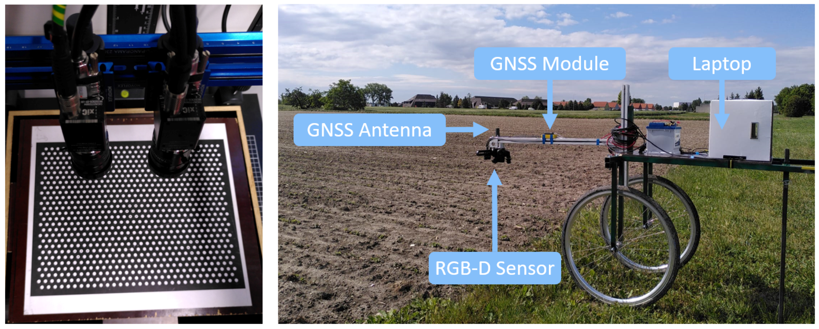
3.2. Acquisition Setup
3.3. Field Trials
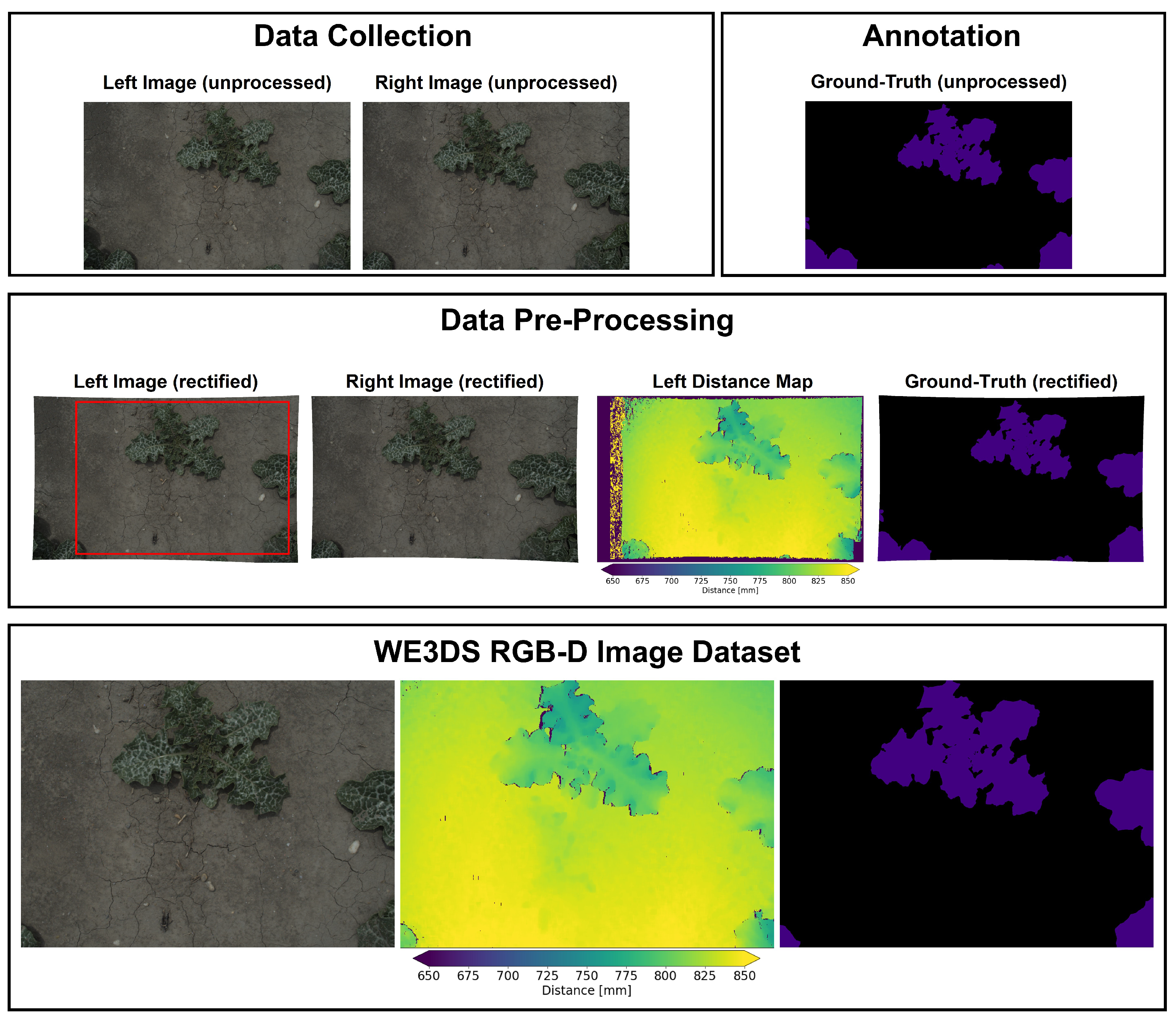
3.4. Data Collection
3.5. Data Pre-Processing
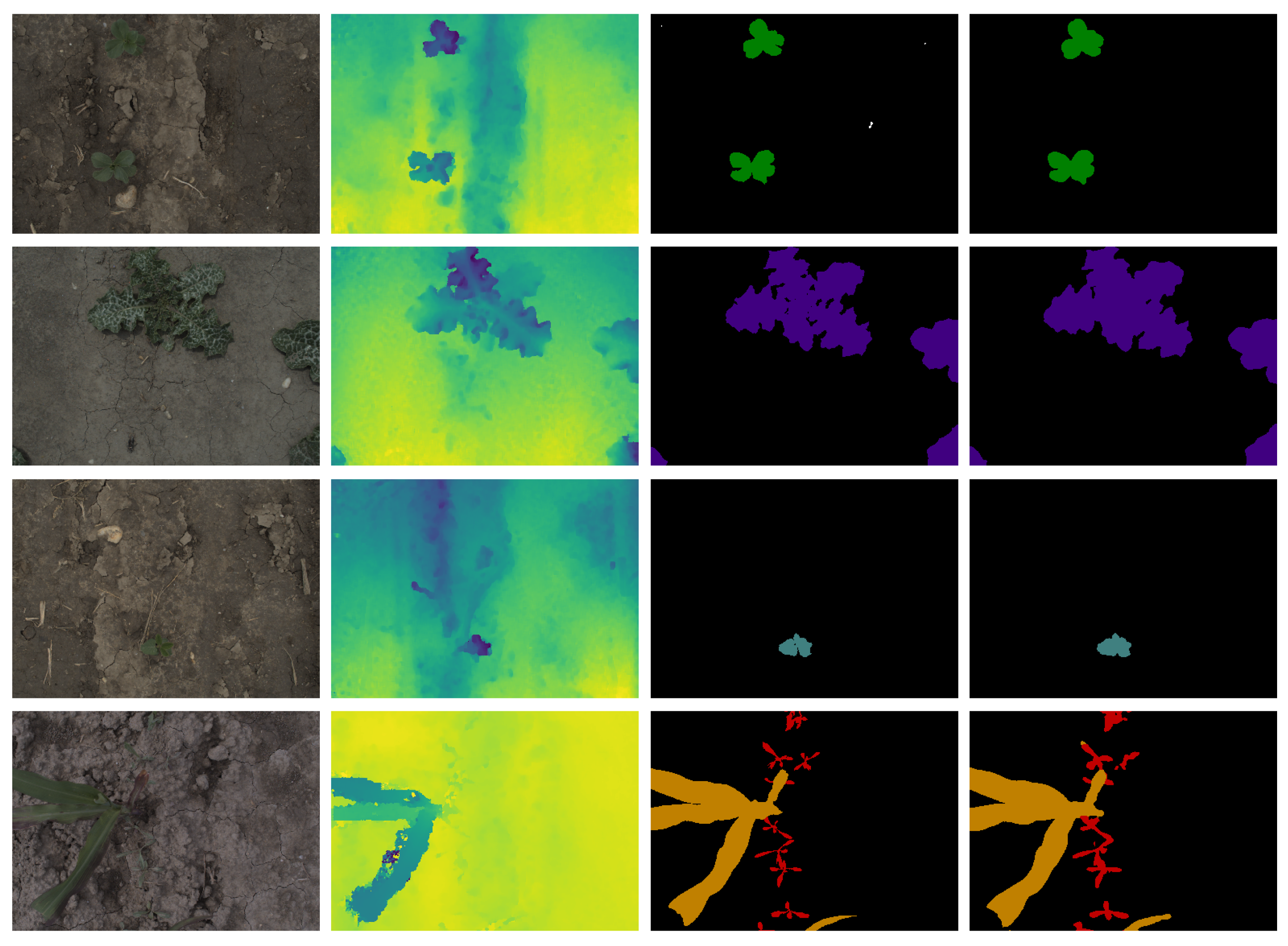
3.6. Ground-Truth Annotation
3.7. Dataset Statistics
3.7.1. Metadata
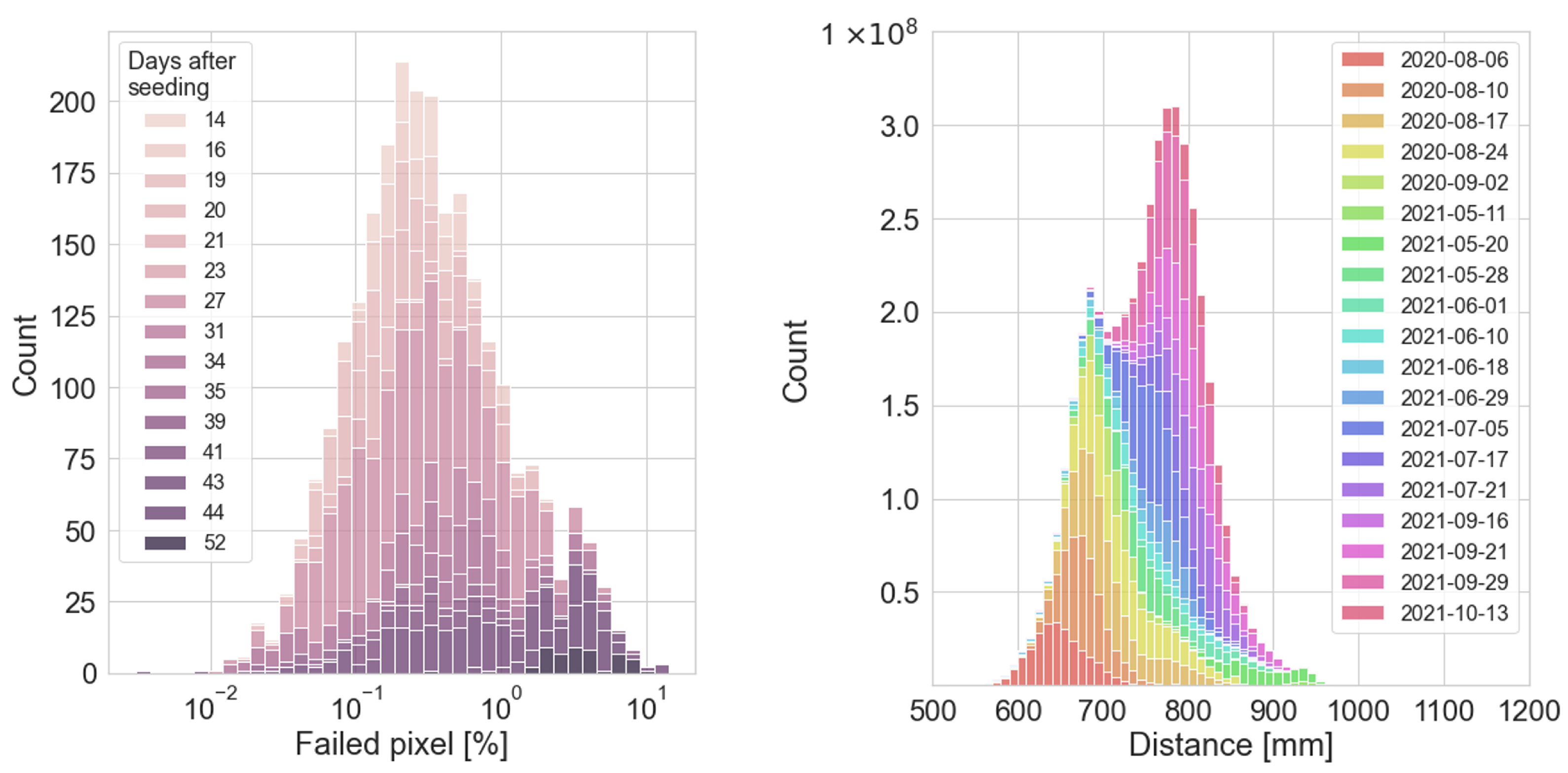
3.7.2. Distance Maps
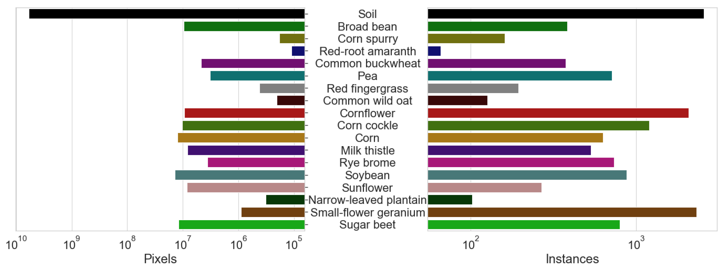
3.7.3. Crop and Weeds Distribution
4. Benchmark
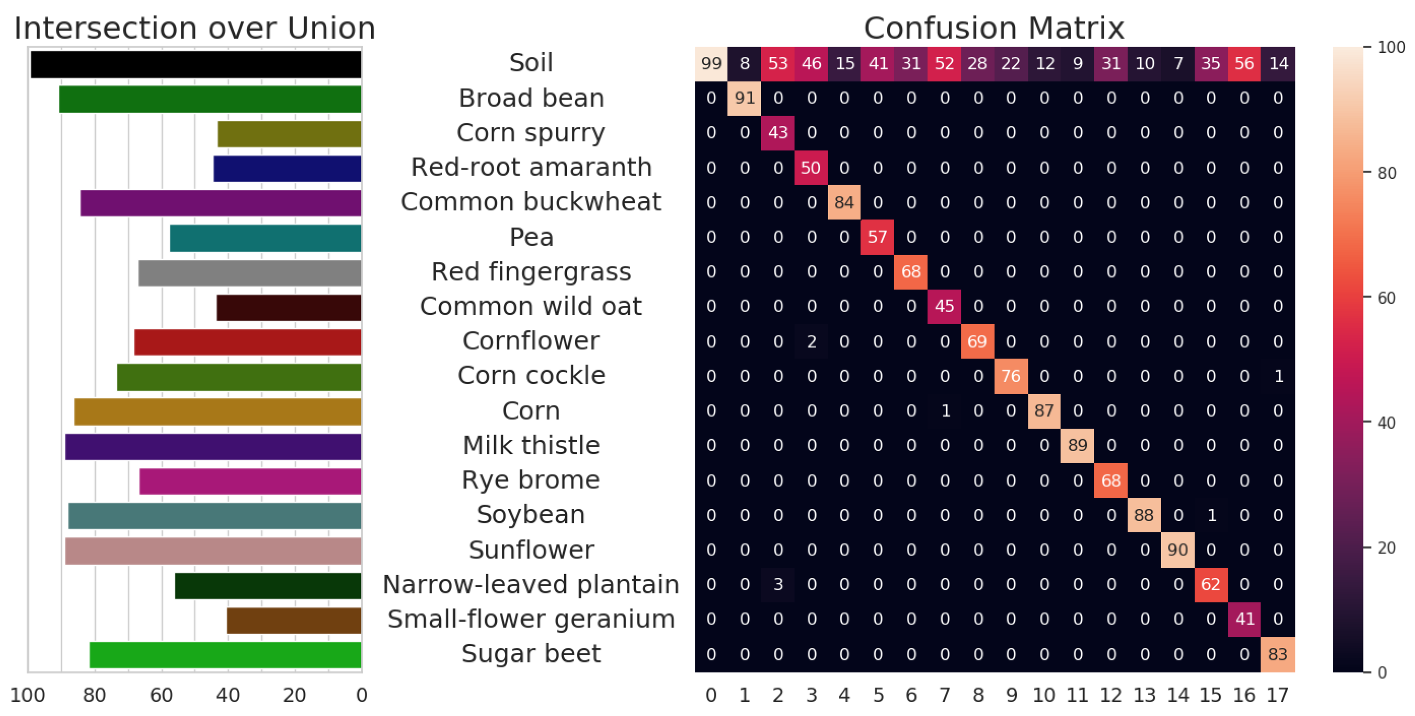
4.1. Task and Metrics
4.2. State of the Art
4.3. Experiments
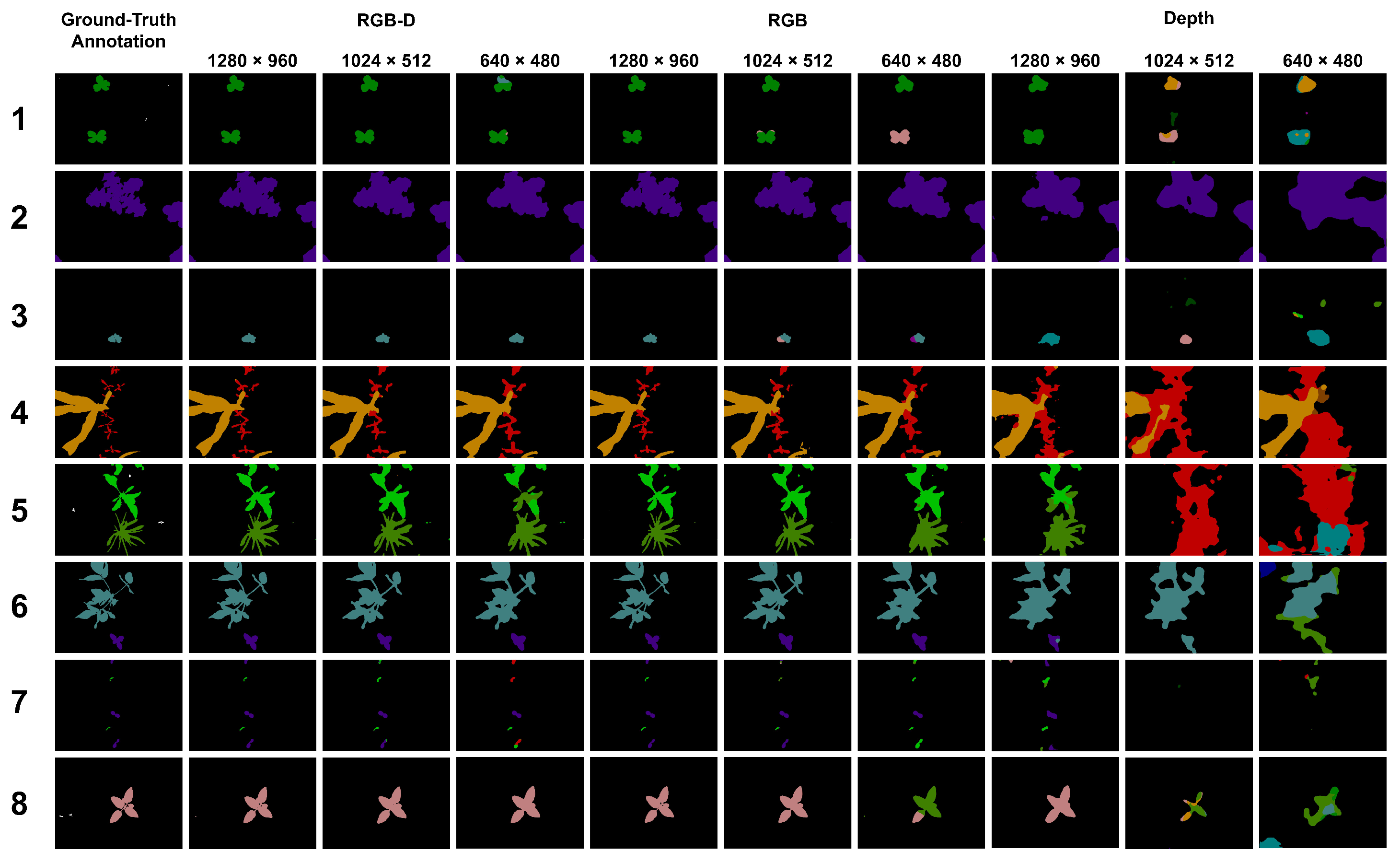
4.4. Results
5. Discussion
6. Conclusions
Supplementary Materials
Author Contributions
Funding
Institutional Review Board Statement
Informed Consent Statement
Data Availability Statement
Acknowledgments
Conflicts of Interest
Abbreviations
| AGV | Automated guided vehicles |
| AMR | Autonomous mobile robots |
| CVAT | Computer vision annotation tool |
| CMOS | Complementary metal-oxide-semiconductor |
| CNN | Convolutional neural network |
| D | Distance map |
| FCN | Fully convolutional network |
| FN | False negatives |
| FP | False positives |
| FPS | Frames per second |
| GNSS | Global navigation satellite system |
| GPIO | General-purpose input/output |
| GPU | Graphics processing unit |
| GUI | Graphical user interface |
| HHA | Depth information as horizontal disparity, height, angle |
| mIoU | Mean Intersection over Union |
| ML | Machine learning |
| MP | Megapixel |
| NCC | Normalized cross-correlation |
| NIR | Near infrared |
| RAM | Random-access memory |
| RGB | RGB color space (red, green, blue) |
| RGB-D | 4-channel image (color, distance) |
| SAD | Sum of absolute gray value difference |
| SF | Smart farming |
| SSD | Sum of squared gray value difference |
| TN | True negatives |
| TP | True positives |
| UAV | Unmanned aerial vehicles |
| UTC | Coordinated Universal Time |
| xiAPI | XIMEA Application Programming Interface |
References
- Kitzler, F.; Wagentristl, H.; Neugschwandtner, R.W.; Gronauer, A.; Motsch, V. Influence of Selected Modeling Parameters on Plant Segmentation Quality Using Decision Tree Classifiers. Agriculture 2022, 12, 1408. [Google Scholar] [CrossRef]
- Sa, I.; Chen, Z.; Popović, M.; Khanna, R.; Liebisch, F.; Nieto, J.; Siegwart, R. weednet: Dense semantic weed classification using multispectral images and mav for smart farming. IEEE Robot. Autom. Lett. 2017, 3, 588–595. [Google Scholar] [CrossRef] [Green Version]
- Shi, W.; van de Zedde, R.; Jiang, H.; Kootstra, G. Plant-part segmentation using deep learning and multi-view vision. Biosyst. Eng. 2019, 187, 81–95. [Google Scholar] [CrossRef]
- Chiu, M.T.; Xu, X.; Wei, Y.; Huang, Z.; Schwing, A.G.; Brunner, R.; Khachatrian, H.; Karapetyan, H.; Dozier, I.; Rose, G.; et al. Agriculture-vision: A large aerial image database for agricultural pattern analysis. In Proceedings of the IEEE/CVF Conference on Computer Vision and Pattern Recognition, Seattle, WA, USA, 13–19 June 2020; pp. 2828–2838. [Google Scholar]
- Too, E.C.; Yujian, L.; Njuki, S.; Yingchun, L. A comparative study of fine-tuning deep learning models for plant disease identification. Comput. Electron. Agric. 2019, 161, 272–279. [Google Scholar] [CrossRef]
- Nørremark, M.; Griepentrog, H.W. Analysis and definition of the close-to-crop area in relation to robotic weeding. In Proceedings of the 6th Workshop of the EWRS Working Group ‘Physical and Cultural Weed Control’, Lillehammer, Norway, 8–10 March 2004; European Weed Research Society: Lillehammer, Norway, 2004. [Google Scholar]
- Auernhammer, H. Precision farming—The environmental challenge. Comput. Electron. Agric. 2001, 30, 31–43. [Google Scholar] [CrossRef]
- Patzold, S.; Mertens, F.M.; Bornemann, L.; Koleczek, B.; Franke, J.; Feilhauer, H.; Welp, G. Soil heterogeneity at the field scale: A challenge for precision crop protection. Precis. Agric. 2008, 9, 367–390. [Google Scholar] [CrossRef]
- Saiz-Rubio, V.; Rovira-Más, F. From smart farming towards agriculture 5.0: A review on crop data management. Agronomy 2020, 10, 207. [Google Scholar] [CrossRef] [Green Version]
- Oerke, E. Crop losses to pests. J. Agric. Sci. 2005, 144, 31–43. [Google Scholar] [CrossRef]
- Norsworthy, J.K.; Ward, S.M.; Shaw, D.R.; Llewellyn, R.S.; Nichols, R.L.; Webster, T.M.; Bradley, K.W.; Frisvold, G.; Powles, S.B.; Burgos, N.R.; et al. Reducing the risks of herbicide resistance: Best management practices and recommendations. Weed Sci. 2012, 60, 31–62. [Google Scholar] [CrossRef] [Green Version]
- Alengebawy, A.; Abdelkhalek, S.T.; Qureshi, S.R.; Wang, M.Q. Heavy metals and pesticides toxicity in agricultural soil and plants: Ecological risks and human health implications. Toxics 2021, 9, 42. [Google Scholar] [CrossRef]
- Heege, H.J.; Thiessen, E. Sensing of Crop Properties. In Precision in Crop Farming; Springer: Dordrecht, The Netherlands, 2013; pp. 103–141. [Google Scholar]
- Melland, A.R.; Silburn, D.M.; McHugh, A.D.; Fillols, E.; Rojas-Ponce, S.; Baillie, C.; Lewis, S. Spot spraying reduces herbicide concentrations in runoff. J. Agric. Food Chem. 2016, 64, 4009–4020. [Google Scholar] [CrossRef] [PubMed]
- Griepentrog, H.W.; Dedousis, A.P. Mechanical weed control. In Soil Engineering; Springer: Berlin/Heidelberg, Germany, 2010; pp. 171–179. [Google Scholar]
- Langsenkamp, F.; Sellmann, F.; Kohlbrecher, M.; Kielhorn, A.; Strothmann, W.; Michaels, A.; Ruckelshausen, A.; Trautz, D. Tube Stamp for mechanical intra-row individual Plant Weed Control. In Proceedings of the 18th World Congress of CIGR, Beijing, China, 16–19 September 2014; pp. 16–19. [Google Scholar]
- Mézière, D.; Petit, S.; Granger, S.; Biju-Duval, L.; Colbach, N. Developing a set of simulation-based indicators to assess harmfulness and contribution to biodiversity of weed communities in cropping systems. Ecol. Indic. 2015, 48, 157–170. [Google Scholar] [CrossRef]
- Bensch, C.N.; Horak, M.J.; Peterson, D. Interference of redroot pigweed (Amaranthus retroflexus), Palmer amaranth (A. palmeri), and common waterhemp (A. rudis) in soybean. Weed Sci. 2003, 51, 37–43. [Google Scholar] [CrossRef]
- Bosilj, P.; Aptoula, E.; Duckett, T.; Cielniak, G. Transfer learning between crop types for semantic segmentation of crops versus weeds in precision agriculture. J. Field Robot. 2020, 37, 7–19. [Google Scholar] [CrossRef]
- Lottes, P.; Khanna, R.; Pfeifer, J.; Siegwart, R.; Stachniss, C. UAV-based crop and weed classification for smart farming. In Proceedings of the 2017 IEEE International Conference on Robotics and Automation (ICRA), Singapore, 29 May–3 June 2017; pp. 3024–3031. [Google Scholar]
- Lottes, P.; Behley, J.; Milioto, A.; Stachniss, C. Fully convolutional networks with sequential information for robust crop and weed detection in precision farming. IEEE Robot. Autom. Lett. 2018, 3, 2870–2877. [Google Scholar] [CrossRef] [Green Version]
- Milioto, A.; Lottes, P.; Stachniss, C. Real-time semantic segmentation of crop and weed for precision agriculture robots leveraging background knowledge in CNNs. In Proceedings of the 2018 IEEE International Conference on Robotics and Automation (ICRA), Brisbane, Australia, 21–25 May 2018; pp. 2229–2235. [Google Scholar]
- Ronneberger, O.; Fischer, P.; Brox, T. U-Net: Convolutional Networks for Biomedical Image Segmentation. In Proceedings of the Medical Image Computing and Computer-Assisted Intervention—MICCAI 2015, Munich, Germany, 5–9 October 2015; Navab, N., Hornegger, J., Wells, W.M., Frangi, A.F., Eds.; Springer International Publishing: Cham, Switzerland, 2015; pp. 234–241. [Google Scholar]
- Lameski, P.; Zdravevski, E.; Trajkovik, V.; Kulakov, A. Weed detection dataset with RGB images taken under variable light conditions. In Proceedings of the International Conference on ICT Innovations, Skopje, Macedonia, 18–23 September 2017; Springer: Cham, Switzerland, 2017; pp. 112–119. [Google Scholar]
- Barchid, S.; Mennesson, J.; Djéraba, C. Review on Indoor RGB-D Semantic Segmentation with Deep Convolutional Neural Networks. arXiv 2021, arXiv:2105.11925. [Google Scholar]
- Seichter, D.; Köhler, M.; Lewandowski, B.; Wengefeld, T.; Gross, H.M. Efficient rgb-d semantic segmentation for indoor scene analysis. In Proceedings of the 2021 IEEE International Conference on Robotics and Automation (ICRA), Xi’an, China, 30 May–5 June 2021; pp. 13525–13531. [Google Scholar]
- Song, S.; Lichtenberg, S.P.; Xiao, J. Sun rgb-d: A rgb-d scene understanding benchmark suite. In Proceedings of the IEEE Conference on Computer Vision and Pattern Recognition, Boston, MA, USA, 7–12 June 2015; pp. 567–576. [Google Scholar]
- Silberman, N.; Hoiem, D.; Kohli, P.; Fergus, R. Indoor segmentation and support inference from rgbd images. In Proceedings of the European Conference on Computer Vision, Florence, Italy, 7–13 October 2012; Springer: Berlin/Heidelberg, Germany, 2012; pp. 746–760. [Google Scholar]
- Silberman, N.; Fergus, R. Indoor scene segmentation using a structured light sensor. In Proceedings of the 2011 IEEE International Conference on Computer Vision Workshops (ICCV Workshops), Barcelona, Spain, 6–13 November 2011; pp. 601–608. [Google Scholar]
- Cordts, M.; Omran, M.; Ramos, S.; Rehfeld, T.; Enzweiler, M.; Benenson, R.; Franke, U.; Roth, S.; Schiele, B. The cityscapes dataset for semantic urban scene understanding. In Proceedings of the IEEE Conference on Computer Vision and Pattern Recognition, Las Vegas, NV, USA, 26 June–1 July 2016; pp. 3213–3223. [Google Scholar]
- Geiger, A.; Lenz, P.; Stiller, C.; Urtasun, R. Vision meets robotics: The kitti dataset. Int. J. Robot. Res. 2013, 32, 1231–1237. [Google Scholar] [CrossRef] [Green Version]
- Brostow, G.J.; Fauqueur, J.; Cipolla, R. Semantic object classes in video: A high-definition ground truth database. Pattern Recognit. Lett. 2009, 30, 88–97. [Google Scholar] [CrossRef]
- Scharwächter, T.; Enzweiler, M.; Franke, U.; Roth, S. Efficient multi-cue scene segmentation. In Proceedings of the German Conference on Pattern Recognition, Saarbrücken, Germany, 3–6 September 2013; Springer: Berlin/Heidelberg, Germany, 2013; pp. 435–445. [Google Scholar]
- Bender, A.; Whelan, B.; Sukkarieh, S. Ladybird Cobbitty 2017 Brassica Dataset; The University of Sydney: Sydney, Australia, 21 March 2019. [Google Scholar]
- Chebrolu, N.; Lottes, P.; Schaefer, A.; Winterhalter, W.; Burgard, W.; Stachniss, C. Agricultural robot dataset for plant classification, localization and mapping on sugar beet fields. Int. J. Robot. Res. 2017, 36, 1045–1052. [Google Scholar] [CrossRef] [Green Version]
- Wu, Z.; Chen, Y.; Zhao, B.; Kang, X.; Ding, Y. Review of Weed Detection Methods Based on Computer Vision. Sensors 2021, 21, 3647. [Google Scholar] [CrossRef]
- Ruckelshausen, A.; Biber, P.; Dorna, M.; Gremmes, H.; Klose, R.; Linz, A.; Rahe, F.; Resch, R.; Thiel, M.; Trautz, D.; et al. BoniRob—An autonomous field robot platform for individual plant phenotyping. Precis. Agric. 2009, 9, 1. [Google Scholar]
- Bender, A.; Whelan, B.; Sukkarieh, S. A high-resolution, multimodal data set for agricultural robotics: A Ladybird’s-eye view of Brassica. J. Field Robot. 2020, 37, 73–96. [Google Scholar] [CrossRef]
- Hensman, J.; Matthews, A.; Ghahramani, Z. Scalable variational Gaussian process classification. In Proceedings of the Artificial Intelligence and Statistics, PMLR, San Diego, CA, USA, 9–12 May 2015; pp. 351–360. [Google Scholar]
- Ren, S.; He, K.; Girshick, R.; Sun, J. Faster r-cnn: Towards real-time object detection with region proposal networks. In Proceedings of the 28th International Conference on Neural Information Processing Systems, Montreal, QC, Canada, 7–12 December 2015. [Google Scholar]
- Chen, X.; Lin, K.Y.; Wang, J.; Wu, W.; Qian, C.; Li, H.; Zeng, G. Bi-directional cross-modality feature propagation with separation-and-aggregation gate for RGB-D semantic segmentation. In Proceedings of the European Conference on Computer Vision, Glasgow, UK, 23–28 August 2020; Springer: Cham, Switzerland, 2020; pp. 561–577. [Google Scholar]
- Couprie, C.; Farabet, C.; Najman, L.; LeCun, Y. Indoor semantic segmentation using depth information. arXiv 2013, arXiv:1301.3572. [Google Scholar]
- Hu, X.; Yang, K.; Fei, L.; Wang, K. Acnet: Attention based network to exploit complementary features for rgbd semantic segmentation. In Proceedings of the 2019 IEEE International Conference on Image Processing (ICIP), Taipei, Taiwan, 22–25 September 2019; pp. 1440–1444. [Google Scholar]
- Jiang, J.; Zheng, L.; Luo, F.; Zhang, Z. Rednet: Residual encoder-decoder network for indoor rgb-d semantic segmentation. arXiv 2018, arXiv:1806.01054. [Google Scholar]
- Park, S.J.; Hong, K.S.; Lee, S. Rdfnet: Rgb-d multi-level residual feature fusion for indoor semantic segmentation. In Proceedings of the IEEE International Conference on Computer Vision, Venice, Italy, 22–29 October 2017; pp. 4980–4989. [Google Scholar]
- Steger, C.; Ulrich, M.; Wiedemann, C. Machine Vision Algorithms and Applications; John Wiley & Sons: Hoboken, NJ, USA, 2018. [Google Scholar]
- Sekachev, B.; Manovich, N.; Zhiltsov, M.; Zhavoronkov, A.; Kalinin, D.; Hoff, B.; Tosmanov.; Kruchinin, D.; Zankevich, A.; Sidnev, D.; et al. opencv/cvat: v1.1.0. 2020. Available online: https://zenodo.org/record/4009388#.Y_bCTHZBxPY (accessed on 1 December 2022).
- Gupta, S.; Girshick, R.; Arbeláez, P.; Malik, J. Learning rich features from RGB-D images for object detection and segmentation. In Proceedings of the European Conference on Computer Vision, Zurich, Switzerland, 6–12 September 2014; Springer: Cham, Switzerland, 2014; pp. 345–360. [Google Scholar]
- Krizhevsky, A.; Sutskever, I.; Hinton, G.E. Imagenet classification with deep convolutional neural networks. In Proceedings of the Advances in Neural Information Processing Systems, Lake Tahoe, NV, USA, 3–8 December 2012; pp. 1097–1105. [Google Scholar]
- He, K.; Zhang, X.; Ren, S.; Sun, J. Deep Residual Learning for Image Recognition. In Proceedings of the IEEE Conference on Computer Vision and Pattern Recognition (CVPR), Las Vegas, NV, USA, 27–30 June 2016. [Google Scholar]
- Deng, J.; Dong, W.; Socher, R.; Li, L.J.; Li, K.; Fei-Fei, L. Imagenet: A large-scale hierarchical image database. In Proceedings of the 2009 IEEE Conference on Computer Vision and Pattern Recognition, Miami, FL, USA, 20–25 June 2009; pp. 248–255. [Google Scholar]
- Badrinarayanan, V.; Kendall, A.; Cipolla, R. Segnet: A deep convolutional encoder-decoder architecture for image segmentation. IEEE Trans. Pattern Anal. Mach. Intell. 2017, 39, 2481–2495. [Google Scholar] [CrossRef]


| Modality | Input [pixels] | mIoU [%] | Inference Frame Rate [FPS] | Training Time [h] | Inference Memory [MB] | Training Memory [GB] |
|---|---|---|---|---|---|---|
| D | 640 × 480 | 14.4 | 38.5 | 42.2 | 33.3 | 6.8 |
| RGB | 640 × 480 | 44.0 | 43.5 | 44.0 | 35.8 | 6.8 |
| RGB-D | 640 × 480 | 48.6 | 26.5 | 63.7 | 51.8 | 10.8 |
| D | 1024 × 512 | 20.6 | 27.0 | 37.7 | 34.2 | 11.5 |
| RGB | 1024 × 512 | 52.4 | 22.2 | 39.2 | 38.4 | 11.5 |
| RGB-D | 1024 × 512 | 59.1 | 19.2 | 85.8 | 55.3 | 18.5 |
| D | 1280 × 960 | 48.5 | 11.3 | 154.1 | 37.0 | 27.1 |
| RGB | 1280 × 960 | 70.1 | 11.0 | 156.1 | 46.8 | 27.1 |
| RGB-D | 1280 × 960 | 70.7 | 8.6 | 240.3 | 66.6 | 43.4 |
| Model | Modality | Dataset | Input [pixels] | mIoU [%] |
|---|---|---|---|---|
| ESANet [26] | RGB-D | NYUv2 | 640 × 480 | 51.6 |
| SA-Gate [41] | RGB-D | SUNRGB-D | 640 × 480 | 49.4 |
| ESANet | RGB-D | WE3DS | 640 × 480 | 48.6 |
| ESANet [26] | RGB | CityScapes | 1024 × 512 | 72.9 |
| ESANet [26] | RGB-D | CityScapes | 1024 × 512 | 75.7 |
| ESANet | RGB | WE3DS | 1024 × 512 | 52.4 |
| ESANet | RGB-D | WE3DS | 1024 × 512 | 59.1 |
| ESANet | RGB | WE3DS | 1280 × 960 | 70.1 |
| ESANet | RGB-D | WE3DS | 1280 × 960 | 70.7 |
| SegNet * [22] | RGB+ | Bonn | 1296 × 966 | 80.8 |
| ESANet [26] | RGB | CityScapes | 2048 × 1024 | 77.6 |
| ESANet [26] | RGB-D | CityScapes | 2048 × 1024 | 78.4 |
Disclaimer/Publisher’s Note: The statements, opinions and data contained in all publications are solely those of the individual author(s) and contributor(s) and not of MDPI and/or the editor(s). MDPI and/or the editor(s) disclaim responsibility for any injury to people or property resulting from any ideas, methods, instructions or products referred to in the content. |
© 2023 by the authors. Licensee MDPI, Basel, Switzerland. This article is an open access article distributed under the terms and conditions of the Creative Commons Attribution (CC BY) license (https://creativecommons.org/licenses/by/4.0/).
Share and Cite
Kitzler, F.; Barta, N.; Neugschwandtner, R.W.; Gronauer, A.; Motsch, V. WE3DS: An RGB-D Image Dataset for Semantic Segmentation in Agriculture. Sensors 2023, 23, 2713. https://doi.org/10.3390/s23052713
Kitzler F, Barta N, Neugschwandtner RW, Gronauer A, Motsch V. WE3DS: An RGB-D Image Dataset for Semantic Segmentation in Agriculture. Sensors. 2023; 23(5):2713. https://doi.org/10.3390/s23052713
Chicago/Turabian StyleKitzler, Florian, Norbert Barta, Reinhard W. Neugschwandtner, Andreas Gronauer, and Viktoria Motsch. 2023. "WE3DS: An RGB-D Image Dataset for Semantic Segmentation in Agriculture" Sensors 23, no. 5: 2713. https://doi.org/10.3390/s23052713