
Pearson Correlation in Determination of Quality of Current Transformers


Abstract
:1. Introduction
- Non-parametric methods are performed in the time domain. Fourier analysis and correlation analysis are used in that case.
- Identification using the parameter estimation procedure uses static variables. This method is characterized by the need to evaluate the initial model, which must be performed in order to obtain convergence towards the final solution. The process is, finally, described by a transfer function.
2. Methodology of CT Accuracy Analysis Using Pearson Correlation Factors and Regression Factors
- The amount “r2” indicates how well the regression line approximates a certain set. It is a percentage value (%) that determines how much of the observed set is within the given variation. It ranges from 0 to 1, i.e., from 0 to 100%.
- The correlation factor “r” is used when one wants to prove the relationship between two variables and the strength of that relationship. It is used with a set of two quantities and ranges from −1 to +1.
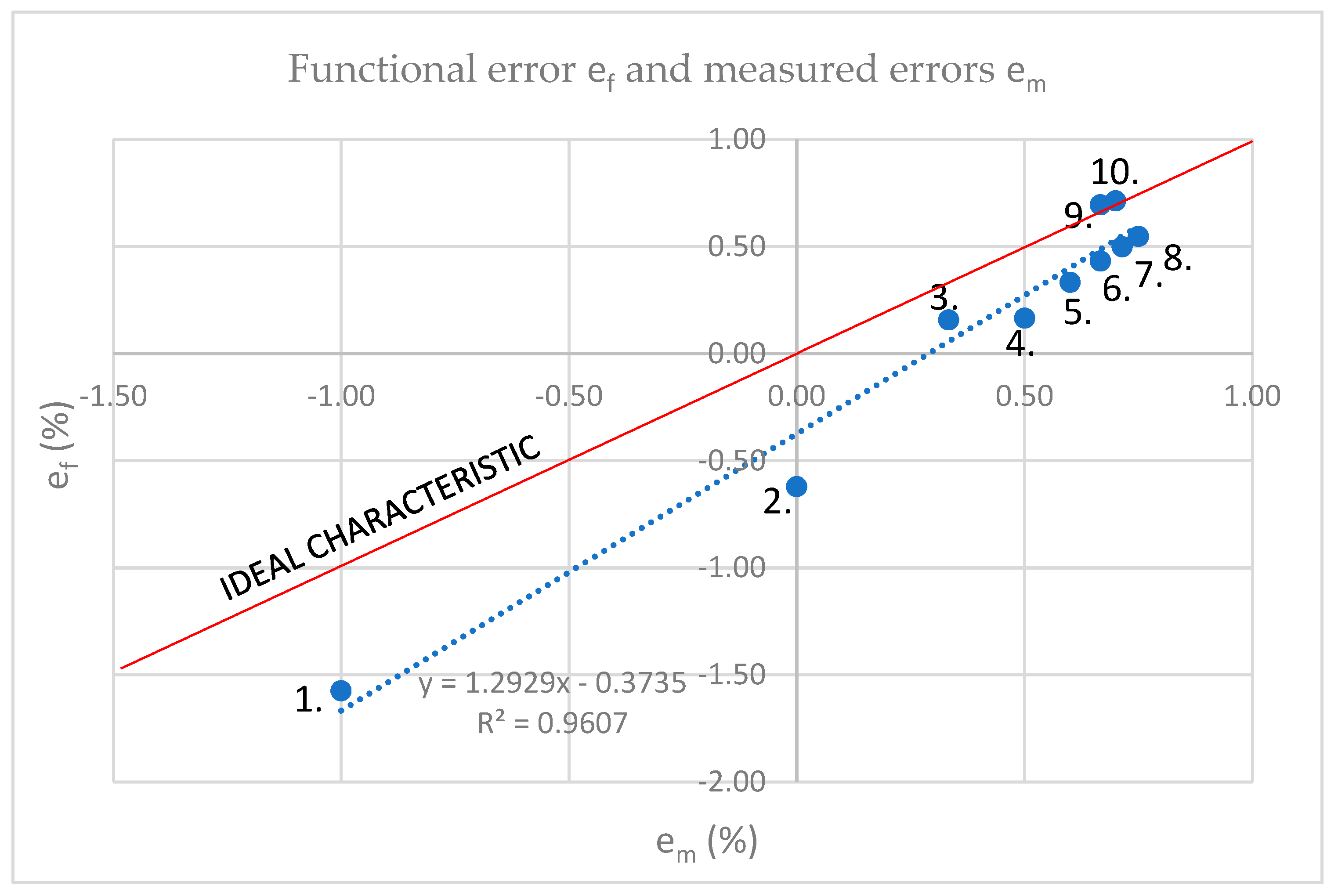
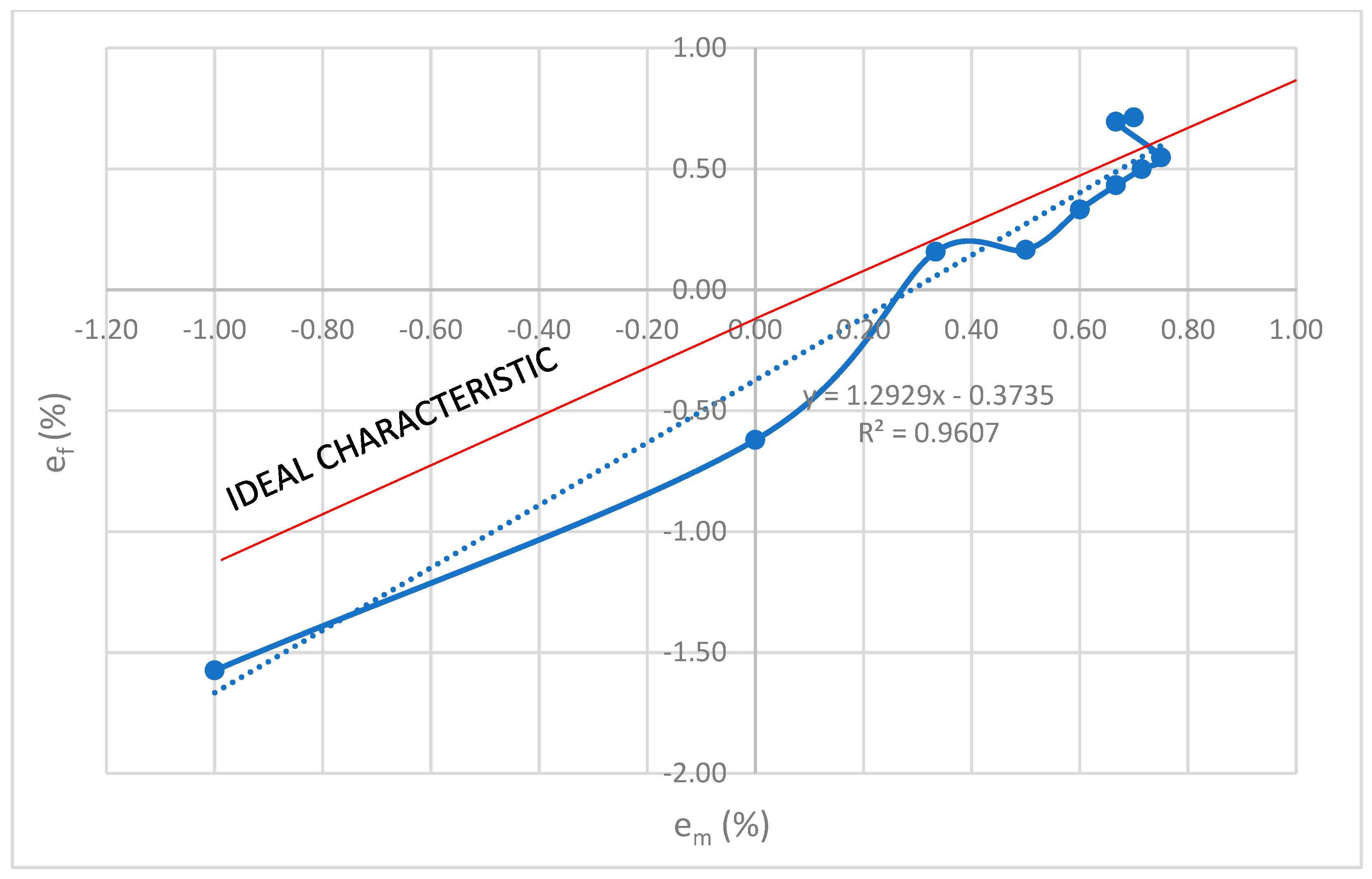
Trajectory Obtained Using “Spline” Interpolation
- visualization of the measurement characteristics of the current transformer
- display of deviations on the entire measuring area
- determination of the place on the curve that contributes to the deterioration of the correlation factor
- insight into the sensitivity of trajectory
- insight into the slope of the trajectory
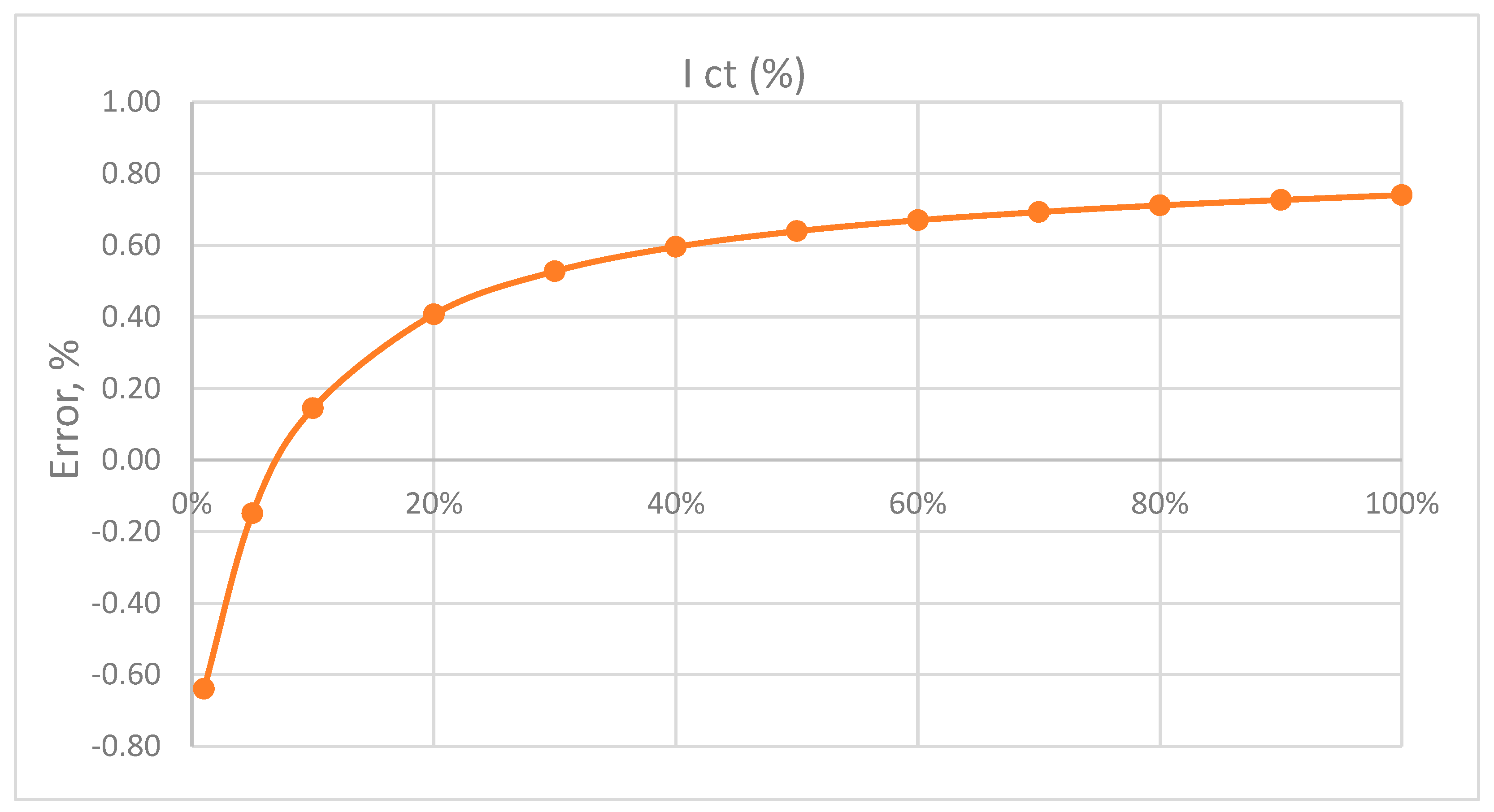
3. Pearson Correlation—Application to the Test
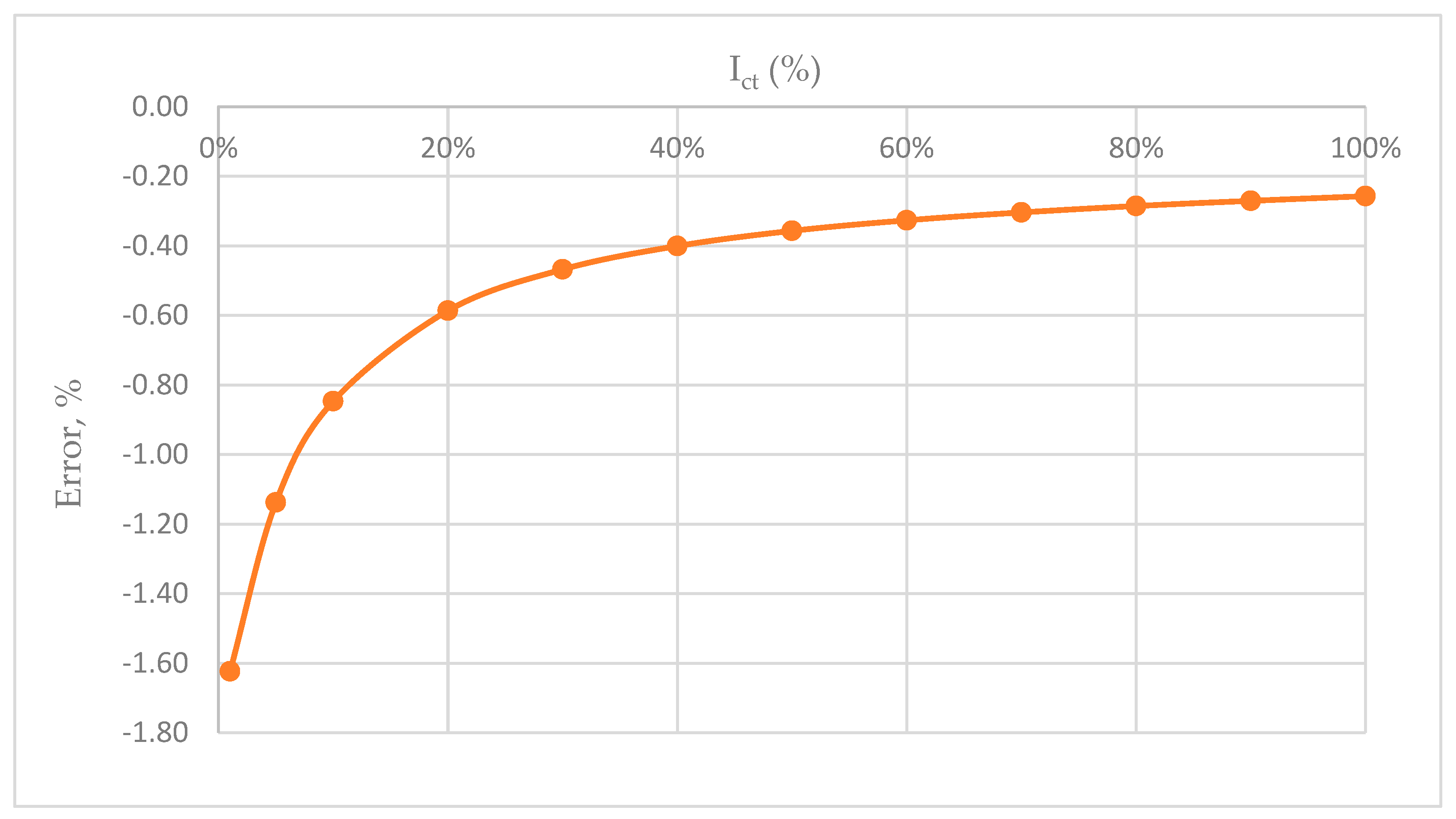
4. Functional Error Analysis of the Current Transformer Transfer Ratio
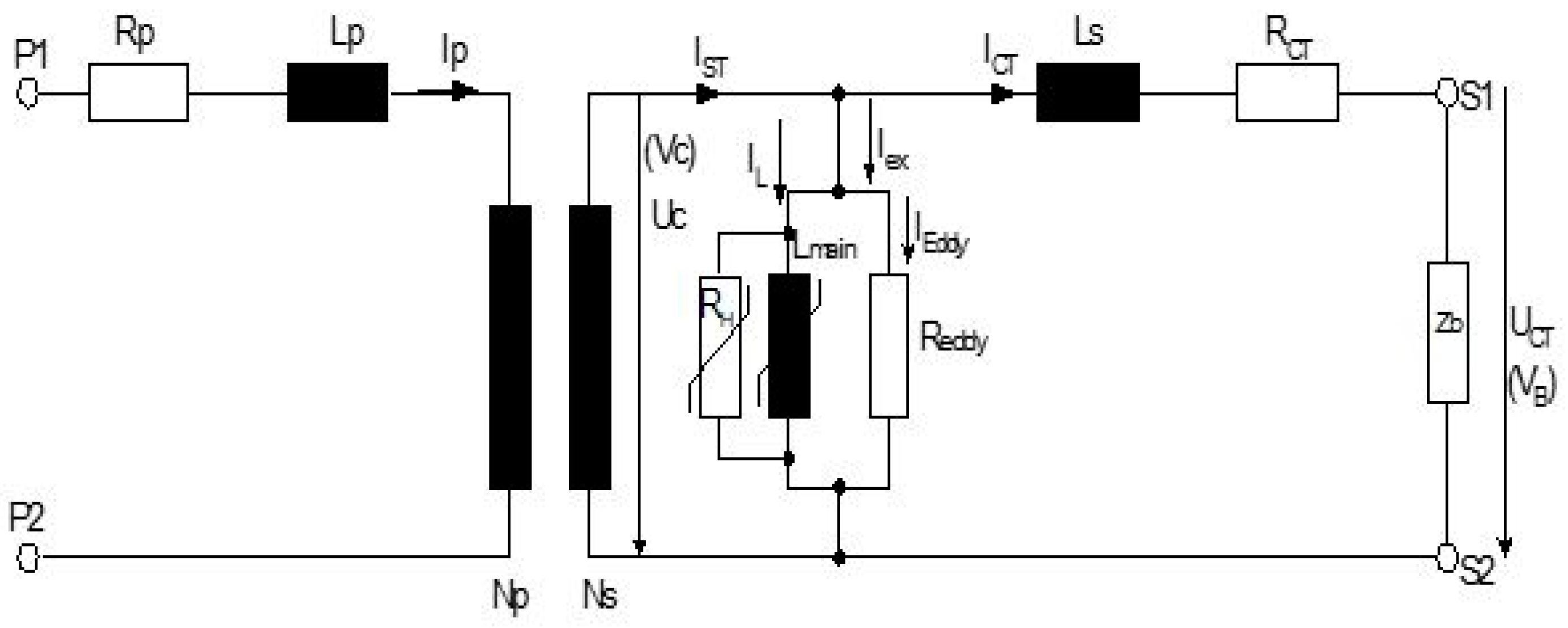
5. Derivation of the Current Transformer Functional Error
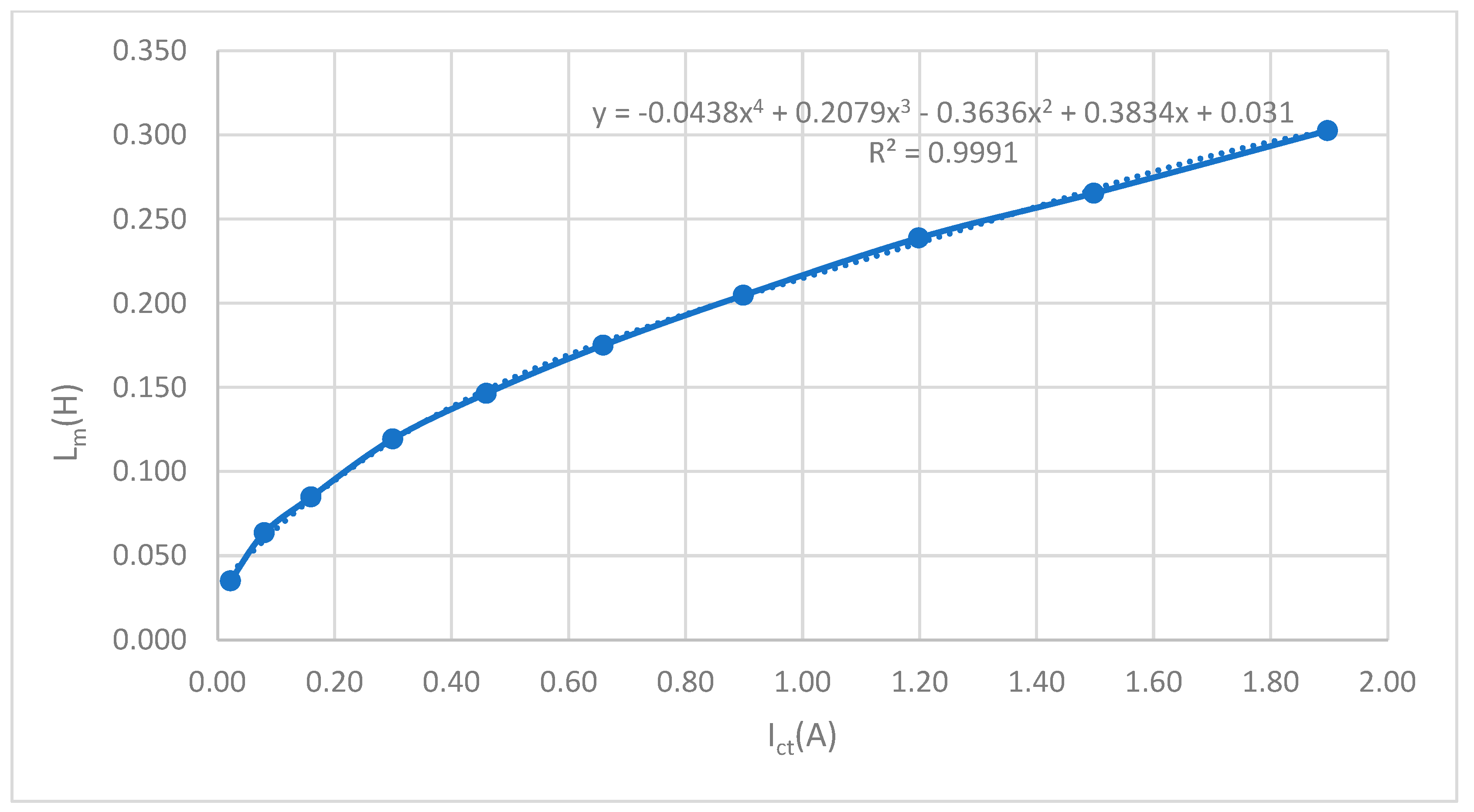
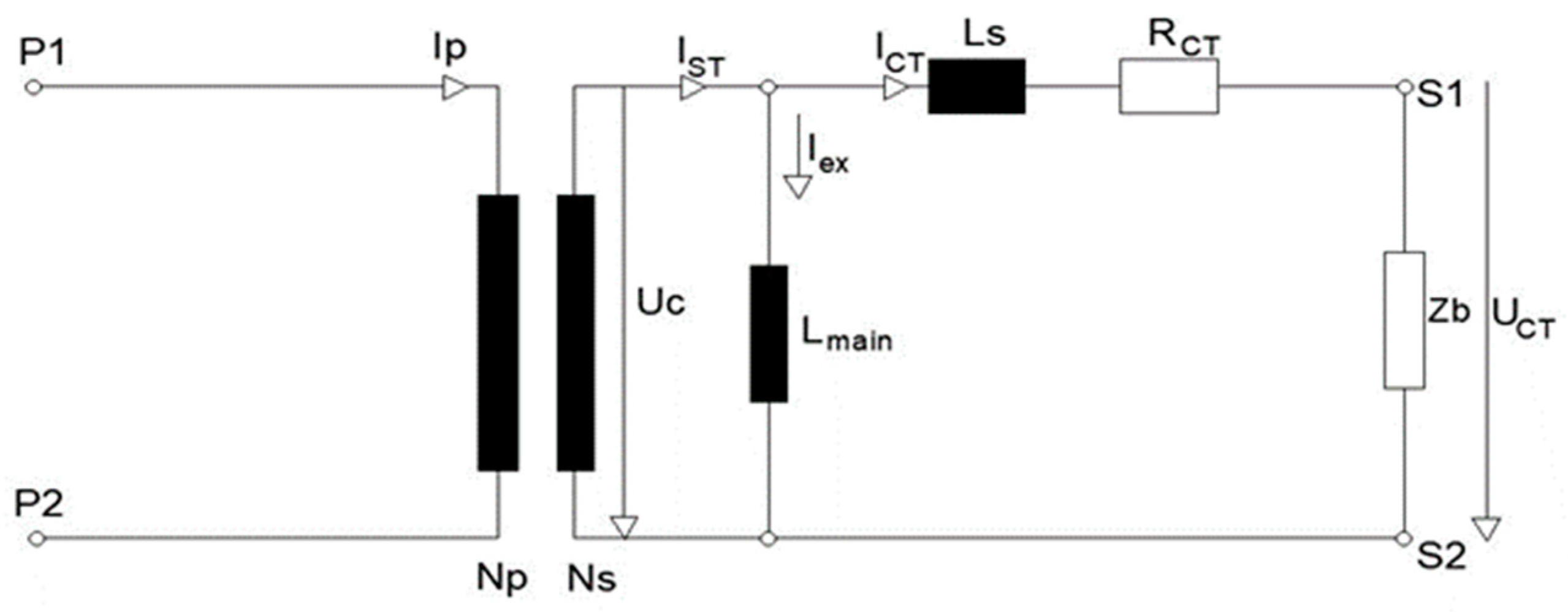
- Lm = secondary inductance Lmain of the current transformer, dependence on the current is given by (1)
- ω = circular frequency
- Rct = ohmic resistance of the secondary
- Ls = inductance of the secondary connection lines
6. Correction of the Number of Secondary Windings
- Lm = secondary inductance Lmain of the current transformer, and dependence on the current is given by (11)
- ω = circular frequency
- Rct = ohmic resistance of the secondary
- Ls = inductance of the secondary connection lines
- nk = corrected number of windings
- n = number of secondary windings
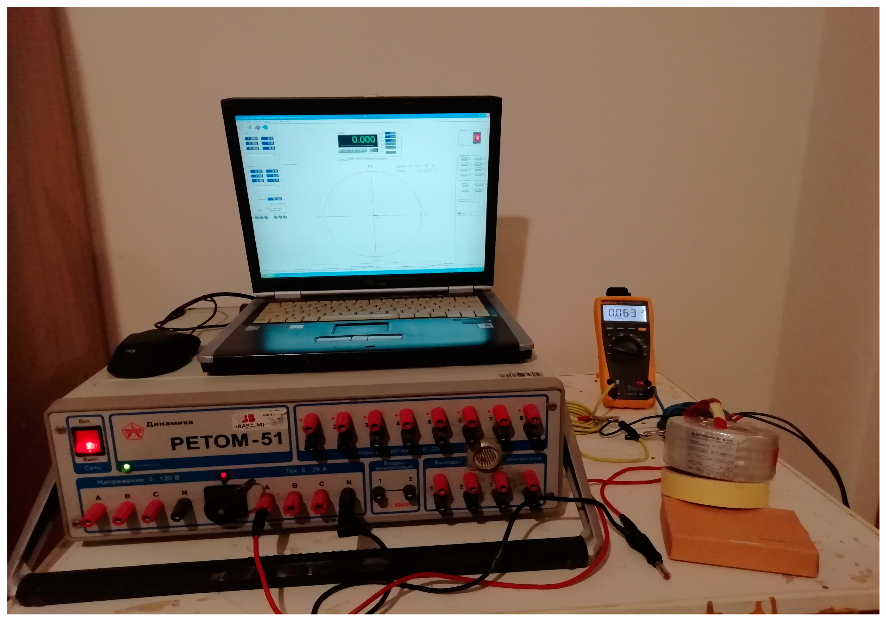
7. Calibration of the Measuring Instrument
- A; constant current source (Amp)
- B = (A/k) · (1 − ε1); “ε1” is functional error of the current transformer, “B” is secondary current of CT, “k” is current ratio
- C = B · (1 − ε2); “ε2” measuring instrument error, “C” is current displayed on ammeter
- C = (A/k) · (1 − ε1) · (1 − ε2) = (A/k) · (1 − ε1 − ε2 + ε1 · ε2) (Amp)
8. Functional Dependence of CT Measurement Error on Temperature
- α = temperature coefficient of electrical resistance, α = 0.00386 1/K
- T0 = initial temperature, 20 °C
- R0 = electrical resistance at temperature T0, R0 = 0.445 Ω
9. Temperature 26.3 °C—Results
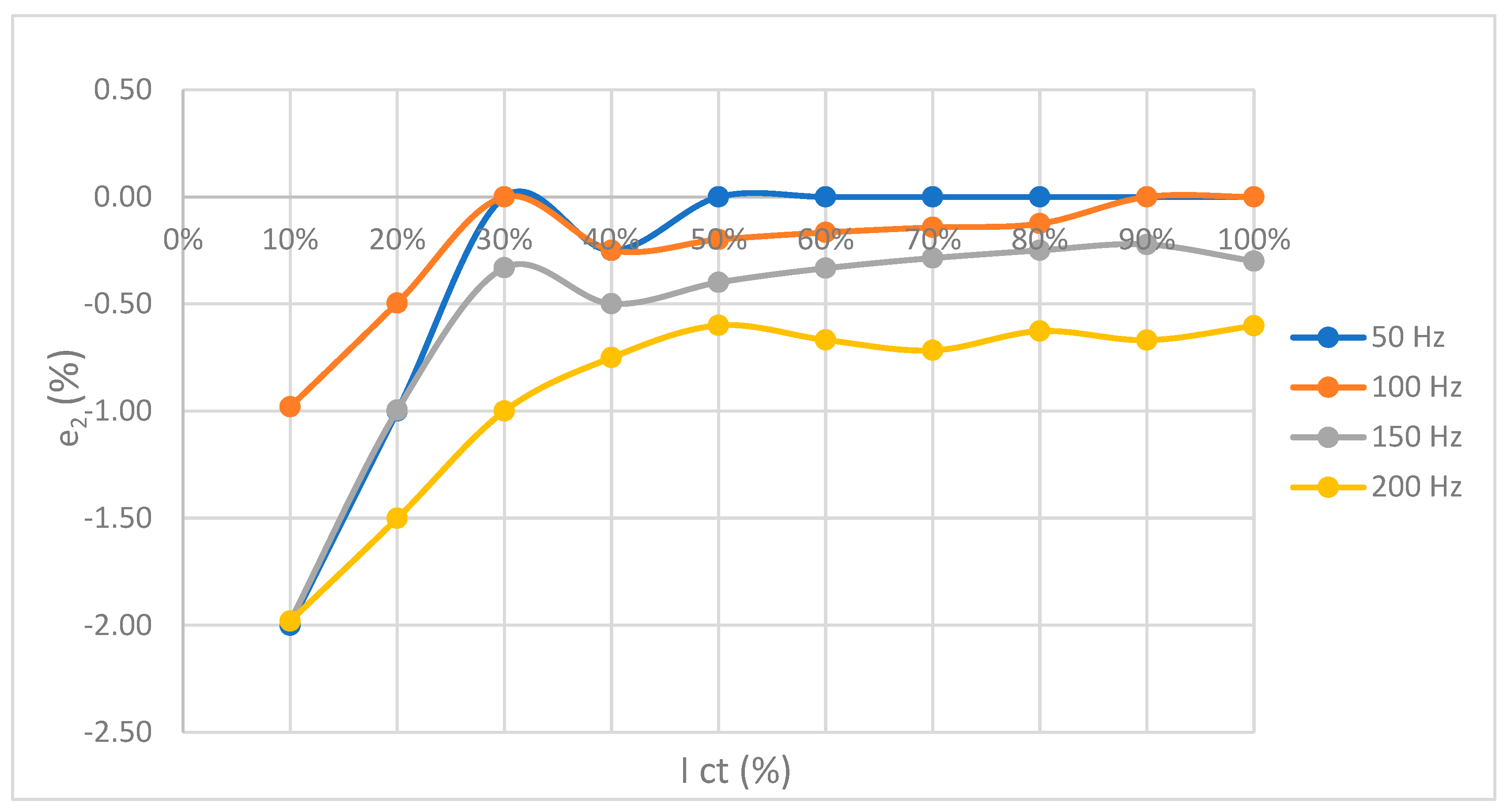
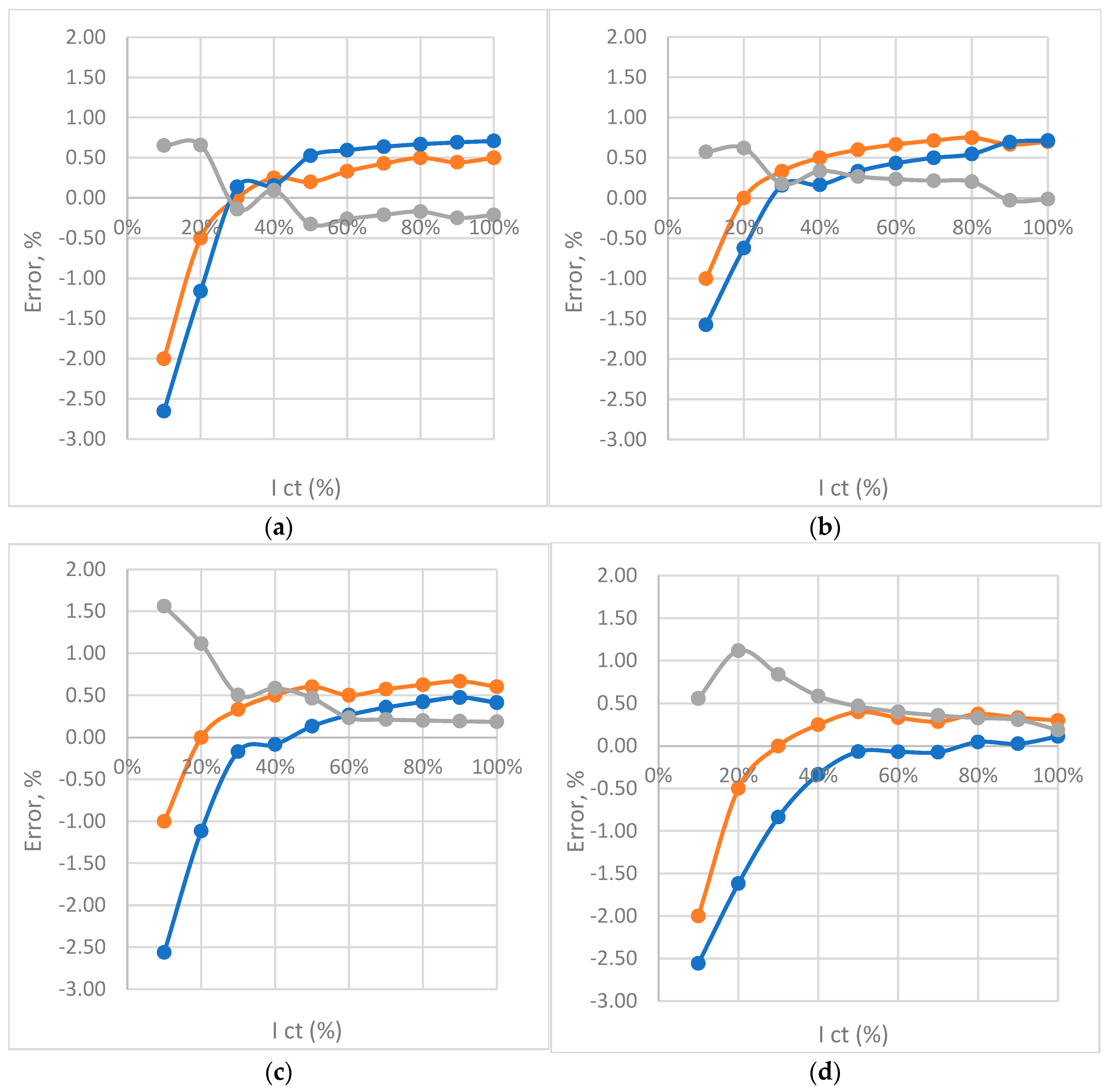
10. Functional Dependence of CT Measurement Error on Frequency
Frequency 50, 100, 150, 200 Hz—Results
11. Discussion about Results of Measurements
12. Partial Correlation of Temperature, Frequency, and CT Measurement Error
- r12–correlation coefficient between the 1st and 2nd variables; r13–correlation coefficient between the 1st i 3rd variables; r23–correlation coefficient between the 2nd and 3rd variables
- r12–correlation coefficient between temperature and frequency, r12 = 0
- r13–correlation coefficient between temperature and CT error, r13 = −0.3137
- r23–correlation coefficient between frequency and error CT-a, r23 = −0.0137
- The influence of frequency on the relationship between temperature and error is r13/2 = −0.3138 (Table 6), which is very close to the correlation of these two quantities, r13 = −0.3137 (Table 5). The conclusion is that the frequency does not influence the relationship between CT error and measurement temperature.
- The influence of temperature on the frequency and CT error is r23/1 = −0.0144 (Table 6), which is very close to the linear correlation of these two quantities, r13 = −0.0137 (Table 5). The conclusion is that temperature has no significant influence on the relationship between CT error and measurement frequency.
- r12/3–partial correlation coefficient between temperature and frequency, r12/3 = 0
- r13/2–partial correlation coefficient between temperature and CT error, r13/2 = −0.3137
- r23/1–partial correlation coefficient between frequency and CT error, r23/1 = −0.0137
13. Conclusions
Author Contributions
Funding
Institutional Review Board Statement
Informed Consent Statement
Conflicts of Interest
References
- CT-Analyzer-Test Ceritficate nr. 111/12/C; Elektrosklop Ltd.: Bestovje, Croatia, 2018.
- Perić, N.; Petrović, I. Identifikacija Procesa—Predavanja; Fakultet Elektrotehnike i Računarstva—Zagreb: Zagreb, Croatia, 2002. [Google Scholar]
- Galić, R. Vjerojatnost i Statistika; Elektrotehnički Fakultet Sveučilišta J.J. Strossmayera u Osijeku: Osijek, Croatia, 1999. [Google Scholar]
- Luchka, A.Y. The Method of Averaging Functional Correction; Academic Press: New York, NY, USA; London, UK, 1963. [Google Scholar]
- Saleh, S.M.; El-Hoshy, S.H.; Gouda, O.E. Proposed diagnostic methodology using the cross-correlation coefficient factor technique for power transformer fault identification. In IET Electric Power Applications; 2017; pp. 412–422. Available online: https://ietresearch.onlinelibrary.wiley.com/doi/pdfdirect/10.1049/iet-epa.2016.0545 (accessed on 17 January 2023).
- Behjat, V.; Mahvi, M.; Rahimpour, E. New statistical approach to interpret power transformer frequency response analysis: Non-parametric statistical methods. In IET Science, Measurement & Technology; 2016; pp. 364–369. Available online: https://ietresearch.onlinelibrary.wiley.com/doi/epdf/10.1049/iet-smt.2015.0204 (accessed on 17 January 2023).
- Herceg, D. Numeričke i Statističke Metode u Obradi Eksperimentalnih Podataka; Institut za Matematiku: Novi Sad, Serbia, 1989. [Google Scholar]
- Yachikov, I.M.; Nikolaev, A.A.; Zhuravlev, P.Y.; Karandaeva, O.I. Estimate of Correlation between Transformer Diagnostic Variables with a Time Lag. Int. Conf. Ind. Eng. ICIE 2017, 206, 1794–1800. [Google Scholar] [CrossRef]
- Wang, X.; Li, Q.; Yang, R.; Li, C.; Zhang, Y. Diagnosis of solid insulation deterioration for power transformers with dissolved gas analysis-based time series correlation. IET Sci. Meas. Technol. 2014, 9, 393–399. [Google Scholar] [CrossRef]
- Guillen, D.; Esponda, H.; Vasquez, E.; Idarraga-Ospina, G. Idarraga-Ospina. Algorithm for transformer differential protection based on wavelet correlation modes. In IET Generation, Transmission & Distribution; 2016; pp. 2871–2879. Available online: https://ietresearch.onlinelibrary.wiley.com/doi/epdf/10.1049/iet-gtd.2015.1147 (accessed on 17 January 2023).
- Yu, T.; Yang, J.; Lin, J.C.; Geng, C. Correlation Analysis of Transformer Parameters Based on Pair-Copula. IOP Conf. Ser. Earth Environ. Sci. 2020, 571, 012005. [Google Scholar] [CrossRef]


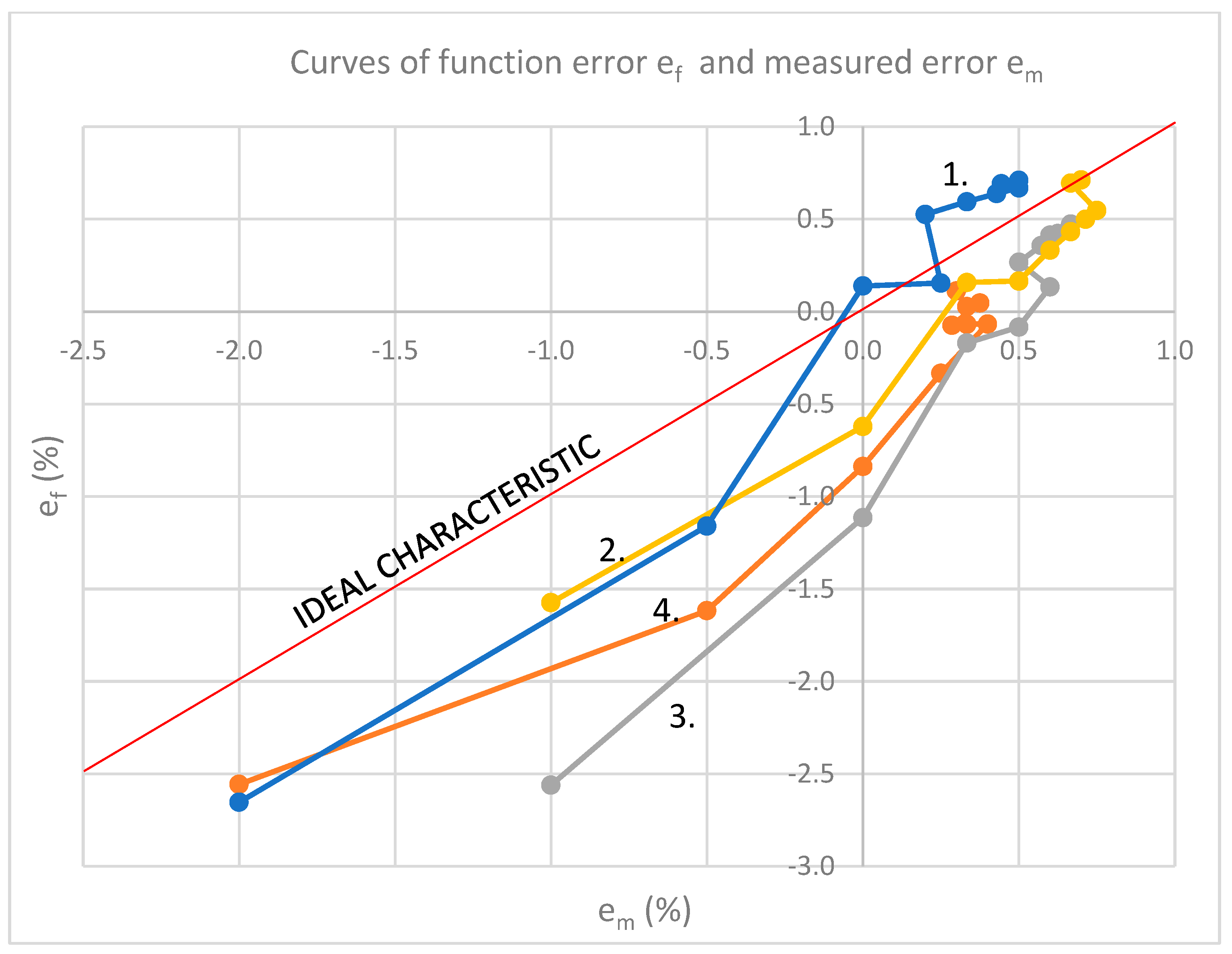
| No. | 1. | 2. | 3. |
|---|---|---|---|
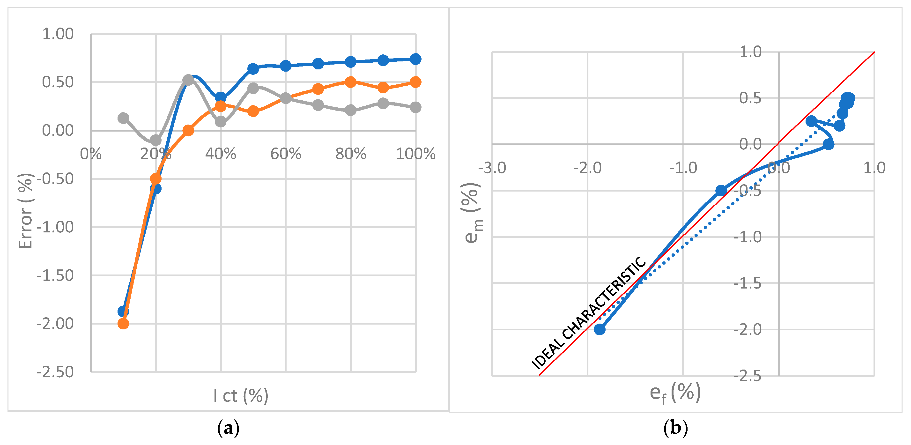
| I (%) | em (%) | ef (%) | |
| 1. | 10% | −1.000 | −1.574 |
| 2. | 20% | 0.000 | −0.620 |
| 3. | 30% | 0.333 | 0.157 |
| 4. | 40% | 0.500 | 0.165 |
| 5. | 50% | 0.600 | 0.332 |
| 6. | 60% | 0.667 | 0.432 |
| 7. | 70% | 0.714 | 0.499 |
| 8. | 80% | 0.750 | 0.547 |
| 9. | 90% | 0.667 | 0.694 |
| 10. | 100% | 0.700 | 0.713 |
| st. dev. s | sx = 0.5126 | sy = 0.6761 |
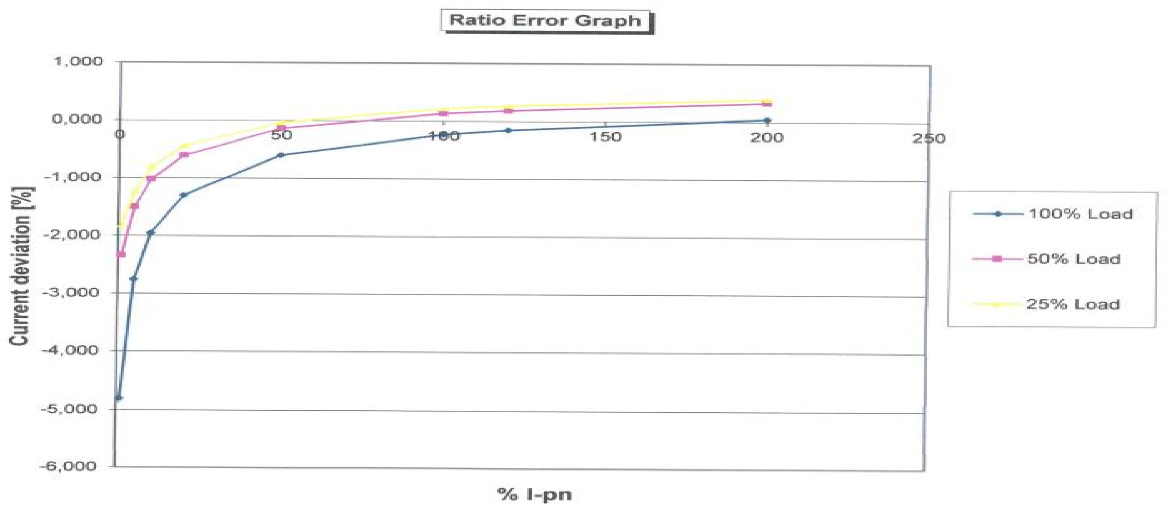
| Nr. | Test Settings | Nr. | Excitation Test | Nr. | Ratio Test | |||
|---|---|---|---|---|---|---|---|---|
| 1 | I-pn | 100 A | 14 | V-kn | 27.663 V | 27 | Ratio | 100:0.99766 |
| 2 | I-sn | 1 A | 15 | V-kn 2 | n.a. | 28 | e | −0.2341% |
| 3 | Rated burden | 2.5 VA/1 | 16 | Ls | 0.0005523 H | 29 | ec | 1.2535% |
| 4 | Operating burden | 2.5 VA/1 | 17 | Kr | 89.07% | 30 | Df | 41.82 min |
| 5 | Applied standard | IEC 61869-2 | 18 | I-kn | 0.088602 | 31 | Polarity | ok |
| 6 | Core type (P/M) | P | 19 | I-kn 2 | n.a. | 32 | N | 99 |
| 7 | Class | 10 P | 20 | Lm | 1.2104 H | |||
| 8 | ALF | 10.0 | ||||||
| 9 | f | 50.0 Hz | nr. | Result with rated burden | ||||
| 10 | Ts | n.a. | 21 | ALF | 11.63 | |||
| 11 | max. Rct | 0.531 W | 22 | Ts | 0.399 s | |||
| 23 | ALFi | 11.4 | ||||||
| nr. | Resistance test | |||||||
| 12 | Rmeas (25 °C) | 0.44532 W | nr. | Result with operating burden | ||||
| 13 | Rref (75 °C) | 0.53112 W | 24 | ALF | 11.63 | |||
| 25 | Ts | 0.399 s | ||||||
| 26 | ALFi | 11.4 | ||||||
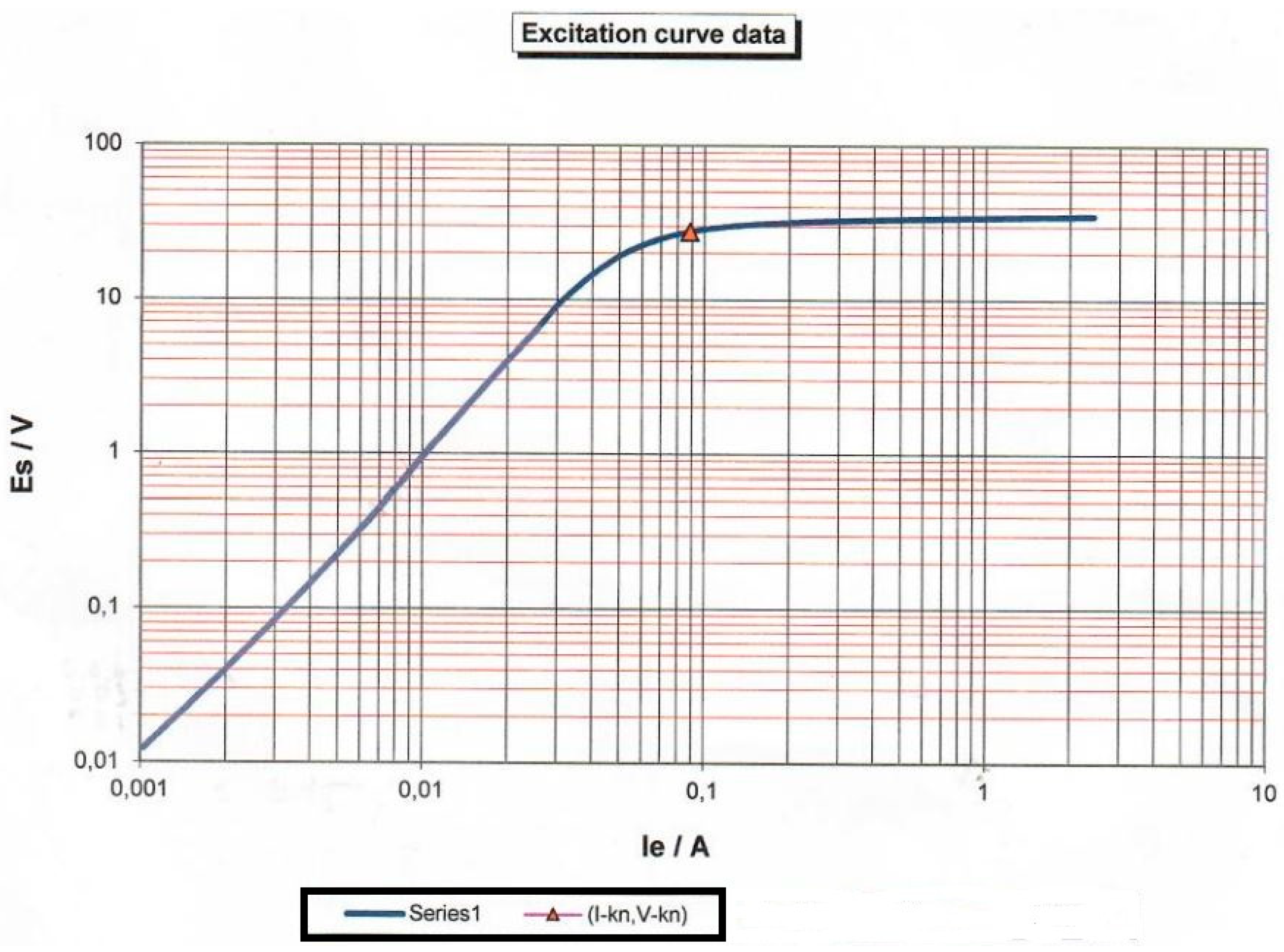
| Ie (A) | 0.001 | 0.002 | 0.003 | 0.004 | 0.005 | 0.006 | 0.007 | 0.008 | 0.009 | 0.01 |
|---|---|---|---|---|---|---|---|---|---|---|
| Es (V) | 0.011 | 0.04 | 0.08 | 0.15 | 0.23 | 0.33 | 0.45 | 0.6 | 0.75 | 0.95 |
| Lm = Es/(Ie·314) (H) | 0.035 | 0.064 | 0.085 | 0.119 | 0.146 | 0.175 | 0.205 | 0.239 | 0.265 | 0.303 |
| |Rct + jwLs| (Ω) | 0.50 | 0.50 | 0.50 | 0.50 | 0.50 | 0.50 | 0.50 | 0.50 | 0.50 | 0.50 |
| Ict = Es/|Rct + jwLs| (A) | 0.02 | 0.08 | 0.16 | 0.30 | 0.46 | 0.66 | 0.90 | 1.20 | 1.50 | 1.90 |
| Point | 1. Segment | 2. I (%) | 3. Ideal Curve SlopeSign | 4. Curve Slope Sign at 50 Hz/ Correlation 3. and 4. | 5. Curve Slope Sign at 100 Hz/ Correlation 3. and 5. | 6. Curve Slope Sign at 150 Hz/ Correlation 3. and 6. | 7. Curve Slope Sign at 200 Hz/ Correlation 3. and 7. |
|---|---|---|---|---|---|---|---|
| 1. | 10% | ||||||
| 2. | 1–2 | 20% | + | +/1 | +/1 | +/1 | +/1 |
| 3. | 2–3 | 30% | + | +/1 | +/1 | +/1 | +/1 |
| 4. | 3–4 | 40% | + | +/1 | +/1 | +/1 | +/1 |
| 5. | 4–5 | 50% | + | −/−1 | +/1 | +/1 | +/1 |
| 6. | 5–6 | 60% | + | +/1 | +/1 | −/−1 | −/−1 |
| 7. | 6–7 | 70% | + | +/1 | +/1 | +/1 | −/−1 |
| 8. | 7–8 | 80% | + | +/1 | +/1 | +/1 | +/1 |
| 9. | 8–9 | 90% | + | −/−1 | −/−1 | +/1 | −/−1 |
| 10. | 9–10 | 100% | + | +/1 | +/1 | +/1 | −/−1 |
| PEARSON CORRELATION “em ∧ ef” | 0.9827 | 0.98 | 0.9862 | 0.957 | |||
| Temp.; R1 | Freq.; R2 | Error CT; R3 | |
|---|---|---|---|
| Temp.; R1 | 1.0000 | 0.0000 | −0.3137 |
| Freq.; R2 | 0.0000 | 1.0000 | −0.0137 |
| Error CT; R3 | −0.3137 | −0.0137 | 1.0000 |
| Freq.; R2 | CT Error; R3 | Temp.; R1 | |
|---|---|---|---|
| Temp/CT Error; R13 | −0.3138 | ||
| Temp/Freq; R12 | −0.0045 | ||
| Freq./CT Error; R23 | −0.0144 |
| Correlation | Value Before Correction | Value After Correction | D% |
|---|---|---|---|
| 1. Temp./CT Error | −0.3137 | −0.3138 | −0.003% |
| 2. Freq./CT Error | −0.0137 | −0.0144 | −5.1% |
Disclaimer/Publisher’s Note: The statements, opinions and data contained in all publications are solely those of the individual author(s) and contributor(s) and not of MDPI and/or the editor(s). MDPI and/or the editor(s) disclaim responsibility for any injury to people or property resulting from any ideas, methods, instructions or products referred to in the content. |
© 2023 by the authors. Licensee MDPI, Basel, Switzerland. This article is an open access article distributed under the terms and conditions of the Creative Commons Attribution (CC BY) license (https://creativecommons.org/licenses/by/4.0/).
Share and Cite
Burgund, D.; Nikolovski, S.; Galić, D.; Maravić, N. Pearson Correlation in Determination of Quality of Current Transformers. Sensors 2023, 23, 2704. https://doi.org/10.3390/s23052704
Burgund D, Nikolovski S, Galić D, Maravić N. Pearson Correlation in Determination of Quality of Current Transformers. Sensors. 2023; 23(5):2704. https://doi.org/10.3390/s23052704
Chicago/Turabian StyleBurgund, Davorin, Srete Nikolovski, Dario Galić, and Nedeljko Maravić. 2023. "Pearson Correlation in Determination of Quality of Current Transformers" Sensors 23, no. 5: 2704. https://doi.org/10.3390/s23052704