Article

A Novel Transformer-Based IMU Self-Calibration Approach through On-Board RGB Camera for UAV Flight Stabilization

1
Department of Computer Science, Sapienza University, Via Salaria 113, 00198 Rome, Italy
2
Department of Mathematics, Computer Science and Physics, University of Udine, Via delle Scienze 206, 33100 Udine, Italy
3
Department of Computer Engineering, Modeling, Electronics and Systems Engineering, University of Calabria, Via Pietro Bucci, 87036 Rende, Italy
*
Author to whom correspondence should be addressed.
Sensors 2023, 23(5), 2655; https://doi.org/10.3390/s23052655
Submission received: 23 December 2022 / Revised: 16 February 2023 / Accepted: 22 February 2023 / Published: 28 February 2023
(This article belongs to the Special Issue Feature Papers in Physical Sensors 2022)

Abstract

:
During flight, unmanned aerial vehicles (UAVs) need several sensors to follow a predefined path and reach a specific destination. To this aim, they generally exploit an inertial measurement unit (IMU) for pose estimation. Usually, in the UAV context, an IMU entails a three-axis accelerometer and a three-axis gyroscope. However, as happens for many physical devices, they can present some misalignment between the real value and the registered one. These systematic or occasional errors can derive from different sources and could be related to the sensor itself or to external noise due to the place where it is located. Hardware calibration requires special equipment, which is not always available. In any case, even if possible, it can be used to solve the physical problem and sometimes requires removing the sensor from its location, which is not always feasible. At the same time, solving the problem of external noise usually requires software procedures. Moreover, as reported in the literature, even two IMUs from the same brand and the same production chain could produce different measurements under identical conditions. This paper proposes a soft calibration procedure to reduce the misalignment created by systematic errors and noise based on the grayscale or RGB camera built-in on the drone. Based on the transformer neural network architecture trained in a supervised learning fashion on pairs of short videos shot by the UAV’s camera and the correspondent UAV measurements, the strategy does not require any special equipment. It is easily reproducible and could be used to increase the trajectory accuracy of the UAV during the flight.

1. Introduction

Nowadays, navigation systems play a key role in different scientific and industrial application contexts, including robotics [1] and autonomous vehicles [2]. However, the recently obtained results in this field show remarkable improvements and precision levels. The localization and the pose estimation of a device can be achieved with multiple strategies and techniques [3,4,5]; anyway, the choice of the involved sensors remains a crucial aspect. For instance, the global positioning system (GPS) [6] is one of the most commonly used systems for localizing and tracking devices. Concurrently, the inertial measurement unit (IMU) [7] can also be exploited due to its adaptive nature: it is accurate enough to identify a person [8], but it can even detect actions [9]. Moreover, the combination of multiple sensors [10] can often offer a noticeable improvement in terms of accuracy and precision. In the specific case of unmanned aerial vehicles (UAVs) [11], numerous tasks can be accomplished thanks to technological advancement, e.g., change detection [12,13], anomaly detection [14,15], and tracking [16,17]. However, there are still some open issues. Some of these may concern incorrect values obtained from the UAV sensors, especially when the device is not expensive. According to [18], for short paths, it is possible to ignore the drift caused by a low-cost IMU. It means that the error is feasible in real-life applications. However, it is only valid when the distance to cover is short; in fact, for long distances, the error propagation can be highly relevant, implying an unmanageable drift in applications where accurate precision is critical. In this context, machine learning (ML) and deep learning (DL) approaches are also feeding the research [19,20]. In the past years, the scholars exploiting transformer-based neural networks [21] caused a shockwave in the DL community due to their simplicity and state-of-the-art performances. Transformers are employed in a wide variety of domains: in natural language processing [22,23,24], computer vision [25,26,27], audio processing [28], and UAV applications [29,30,31]. Although the transformer-based networks are currently the standard in many tasks, their downside lies in the energy drain [32], the required computational power, and the needed primary memory, which is quadratic in the number of inputs for attention-based transformers [21].

2. Related Work

To the best of our knowledge, none of the works in literature treats the analyzed task with the same approach proposed in this paper. However, numerous similar applications inspired the presented strategy for a camera-based IMU self-calibration for UAVs.
One of the most relevant works considered in our analysis is [33], where the authors proposed an online IMU self-calibration method for visual–inertial systems equipped with a low-cost inertial sensor. It is specifically designed for unmanned ground vehicles (UGV), but it involves both IMU and camera sensors. It aims to locate the device as accurately as possible. In the first step, the IMU measurements and the camera frames are mapped. Since the image frequency is lower than the IMU updates, the IMU measurements between the two frames are pre-integrated into a single compound measurement. An optimization of the IMU intrinsic parameters is proposed to minimize the errors constrained by the pre-integration measurements. It is achieved by computing a Jacobian matrix [34] for each pre-integration part and estimating the uncertainty of the pre-integration measurements. The final step consists in defining the IMU intrinsic parameters residual. The authors propose an approach in which they are assumed to be uncertain, but which is constant in the time span of the sliding window. The proposed system can be classified as a monocular visual–inertial system (VINS-Mono) [35]. The results obtained on several datasets [36,37,38,39,40] show outstanding results in terms of tracking accuracy and also computational times.
IMU/camera calibration strategies can also be applied in other application areas [41] than those entailing UGVs or UAVs. It suggests that this approach can be considered a valid procedure, even if it seems uncommon. In the specific field of UAVs, it is possible to find different techniques in the recent literature, from the fusion of sensors [42] to the self-calibration [43,44]. For instance, in [45], the authors propose a novel method for monitoring a UAV with a custom-made positioning module that exploits a fusion algorithm. The work explains how the module should be calibrated to reduce the influence of deterministic errors on the IMU. The authors highlight five variables that are correlated to the noise factors on accelerometers and gyroscopes: direct measures, reference excitation acceleration, statistic bias, scale factor, and non-orthogonality. Based on these assumptions, the proposed method exploits a turnable platform to make a specific accelerometer’s axis point to gravity to obtain an output excitation, and it also rotates at a constant angular rate on a specific gyroscope’s axis for the same aim. After the measured output and reference excitation have been acquired, a least-squares method calculates the deterministic errors parameter. Similarly, the deterministic errors of the magnetometer are influenced by multiple factors. The correlated variables are the measured output, the matrix that contains errors like soft iron coefficients and non-orthogonality, the vector of static bias and hard iron coefficients, and the environment magnetic field distribution. The authors noticed how those parameters could provide an equation of a classical vector form of an ellipsoid formula; with an ellipsoid fitting, the geometry parameter can be acquired to calibrate the sensor. Concerning stochastic error identification, three noises have been highlighted: white noise, exponentially correlated noise, and rate random walk. The authors treated them by exploiting the Allan variance method and its accuracy approximation. Then, with system equations, the sixteen states, including attitude, velocity, position, and angle/velocity increment bias, are managed. A Kalman filter-based technique is introduced, in which measures and predictions support each other. The provided steps run to a fusion algorithm that combines all the sensors’ data with the extended Kalman filter approach and provides a more accurate real-time attitude, velocity, and position of the UAV.
Another example of multi-sensor calibration for UAVs is provided in [46], where the authors propose a correction method that involves different GPS sensors, a LIDAR, and an IMU. In the pipeline, three branches are shown: bore sight, time delay, and level arm calibrations. The first one aims to know exactly the relative position of sensors (multiple GPS, IMU, and LIDAR) with respect to each other. The authors provide a method for generating the coordinate transform of these sensors with respect to the center of the drone. Concerning the bore sight calibration, it is used to determine the differences in the rotations of each sensor. The proposed algorithm provides the alignment of the extracted and pre-processed point cloud data from the LIDAR, as well as a comparison with the GPS signals (that are considered the ground truth). It is also specified that the calibration could be even more precise if the IMU is also involved. The time delay calibration deals with the calculation of error-corrected signals. In particular, it refers to the delay in GPS sending and receiving messages. The solution consists in always adding the retrieved error to the location shown by the GPS receiver.
There are also works [47,48,49,50] in which the IMU’s calibration does not require any correlation with other sensors. As expected, most of the recent studies involve machine and deep learning-based techniques. For instance, in [51], the authors propose a calibration method based on deep learning for micro electro mechanical system (MEMS) IMU gyroscopes. The network calibrates the error from the raw data of the MEMS IMU and regresses gyroscope data after the error compensation. During the training, the network output is used to estimate the quaternion and calculate the loss function. During the test phase, the obtained output is exploited for navigation to obtain the altitude and position of the carrier. The results show that the position and the altitude are significantly adjusted by the proposed calibration method, providing relevant scientific soundness of the self-calibration approaches in this application field. Another example is provided by [52], where the introduction of an adaptive neuro-fuzzy inference system (ANFIS) is proposed to improve the effectiveness of low-grade IMUs by estimating and compensating the measurement errors. The method combines the artificial neural network (ANN) with the fuzzy inference system (FIS) and is trained by adding noise to reference IMU data. The proposed solution shows a high correction impact on the considered dataset, highlighting the quality of the strategy.
Concerning the specific deep learning technique of transformers, there are only a few works in the literature featuring this architecture in a UAV-based calibration task. The networks proposed in [53], one based on a long–short term memory (LSTM) architecture [54] and another on a transformer [21], estimating the bias in the sensors involved in the visual–inertial odometry in case of complete absence of visual information. Moreover, ref. [55] proposes a transformer-based architecture to pre-process and clean the IMU measurements before even being used in a flight. These cases suggested that the transformers seem promising in this application area and could provide noticeable improvements when correctly exploited.

3. Proposed Method

The model predicts the offset in the IMU of the drone given an input sequence F R n × h × w of n frames with height h, width w, and a sequence of aligned IMU measurements I R n × 6 , containing records of accelerometer and gyroscope, each along the three axes. The first issue involves synchronization, which can be achieved by exploiting the IMU and the camera timestamps. However, it is worth considering that IMUs have a much higher sampling rate with respect to cameras and that these timestamps could not be perfectly matched. To address this issue, the practical solution is to match each camera frame with the closest corresponding IMU measurement in time. This also has some side effects. On one hand, it reduces the number of inputs for the model, thereby reducing the computational demand. On the other hand, this also ensures that IMU measurements are sampled at the same rate as cameras. This is a practical advantage since it makes the system scalable with the camera quality. To handle the multi-modal nature of the task, the model entails three blocks: a video reducer block (VRB) (Section 3.1) that aims to reduce the input sequence of consecutive frames into an equally long sequence of token vectors; an IMU reducer block (IRB) (Section 3.2) that projects each IMU vector, containing records of accelerometer and gyroscope in each instant of time, into a sequence of token vectors; and a noise predictor block (NPB) (Section 3.3), which merges the information from video and IMU records and predicts the amount of offset in the latter. Figure 1 depicts the model’s architecture. The source code of the presented strategy can be found at https://github.com/rom42pla/rgb2imu_error_estimation.

3.1. Video Reducer Block

This module, whose architecture is shown in Figure 1 and is partially inspired by [26,27], takes as input a sequence of n frames from a video and transforms each frame into a d-dimensional vector, called token, that can be merged with those returned by the IRB for the final prediction. In this context, the video can be grayscale, with F R n × h × w or RGB, with F R n × 3 × h × w . The model is compatible with any combination of n, h, and w.
If a frame F is RGB, it is cast to a single channel via a small convolutional neural network (CNN) C C N χ : R n × 3 × h × w R n × h × w , including a three-dimensional convolution parameterized by χ , an activation function σ and a batch normalization layer [56]:
C N N χ ( F ) = b a t c h n o r m ( σ ( c o n v 3 d χ ( F ) ) ) .
To ensure the preservation of the original information of each image, the output of the CNN is summed with the grayscale version of F as it is usually executed in residual networks [57]:
F = F F is sin gle channel , g r a y s c a l e ( F ) + C N N χ ( F ) F is RGB .
Consequently, each frame is unfolded into a series of p smaller patches of shape h p × w p , yielding a matrix P R n × p × h p × w p . If h is not divisible for h p , or w is not divisible for w p , the frames will be 0-padded (In this context, the image padding consists in adding extra pixels to perform an operation that requires a specific image shape. In a 0-padded image, the pixels added by the padding operation have an intensity of 0 on each channel.) until they fit the legal size for the unfolding operation. Each patch is then flattened into a ( h p · w p ) -dimensional vector to be projected by a feed-forward network (A feed-forward network is often made of a sequence of one or more linear layers and activation functions. Moreover, also, other layer types, such as dropout [58] and normalization [56,59], can often be added, as well, depending on the context.) (FFN) into a d-dimensional token. This FFN, called F F N Θ : R p × ( h p · w p ) R p × d , entails a linear layer, also called fully connected, parameterized by a weights matrix W Θ R d × ( h p · w p ) and a bias vector b Θ R d . There are also an activation function σ and a dropout layer [58] for regularization purposes:
T p = F F N Θ ( P ) = d r o p o u t ( σ ( f l a t t e n ( P ) W Θ T + b Θ ) ) .
After applying F F N Θ individually to each of the n frames, the result will be a sequence of tokens T p R n × p × d .
The token of each patch is then provided to a transformer encoder to exploit the spatial dependencies between the patches. For each frame, it outputs a single token bearing the meaningful learned features towards the task. The transformer encoder architecture is analogous to the one originally presented in [21]. This module is made of a stack of one or multiple transformer encoder layers, which contain a sequence of multi-head attention (MHA) and an FFN with skip-connections. A skip-connection technique consists in using the output of a layer as input for another one placed later in the architecture. This method is commonly exploited in very deep networks to mitigate the vanishing gradient phenomenon [60]. The output of both the MHA and the FFN is further processed by a normalization layer [56,59]. A dot-product attention function takes three inputs Q R n q × d q , K R n v × d k , V R n v × d v , called query, key, and value, and is parameterized by three weights matrix W q R d q × d , W k R d k × d , and W v R d v × d :
A t t e n t i o n ( Q , K , V ) = s o f t m a x Q W q ( K W k ) T d k V W v ,
where W q , W k , and W v are used to transform the three inputs Q, K, V into a single output of shape R n q × d . Therefore, the output of the attention function is a weighted sum of the values V based on the similarity between the query Q and the keys K. A MHA is a projection of the concatenation of the outputs of k dot-product attention operations, parameterized by different weights. The concatenation of the outputs of the attention operations is projected into a smaller space by a learned weight matrix W o R d · k × d :
M H A ( Q , K , V ) = i = 1 k A t t e n t i o n i ( Q , K , V ) W o .
In a transformer encoder, the inputs of the attention functions are all equal to the input matrix, thus Q = K = V . In the VRB, there are multiple instances of the same transformer encoder T E Λ : R p × d R p × d . Each one is fed with the patches of a single frame summed with E Λ R p × d , a matrix of the learned positional embeddings. This is required since the attention Formula (4) does not model positional information [61] and cannot distinguish between patches in different positions. The output of a transformer encoder is a matrix of the same shape as the input, from which the model extracts the first row where all the meaningful information of the frame is squeezed, leading to a sequence of tokens T p ( enc ) R n × d :
T p ( enc ) = T E Λ ( T p + E Γ ) ,
where, T p ( enc ) is further summed with the learned temporal embeddings E Γ R n × d and fed to a transformer encoder T E Γ : R n × d R n × d to transform T p ( enc ) into the output T v ( enc ) R n × d of the VRB. This allows analyzing the temporal relationships between tokens:
T v ( enc ) = T E Γ ( T p ( enc ) + E Γ ) .

3.2. IMU Reducer Block

This module, whose architecture is shown in Figure 1, takes as input a sequence of n IMU measurements I R n × 6 and transforms each of them into a d-dimensional vector, called a token. Each measurement is time-aligned with the corresponding video frames. Although this paper considers 6 typologies of values in the formulations, the model is compatible with any combination of standard IMU measurements to accommodate any device. For instance, if records from both the accelerometer and gyroscope are present in I, then its last dimension will be 6, since three values are for the axes of the accelerometer and three for the gyroscope. Meanwhile, as in the case of the experiments on the Zurich MAV dataset [39], if the measurements of only the axes of one of the two sensors are available, I will contain n × 3 values.
The measurements I are processed by F F N Ξ : R n × 6 R n × d , entailing two linear layers, respectively, parameterized by W Ξ , 1 , b Ξ , 1 and W Ξ , 2 , b Ξ , 2 , to project these vectors into the same space of the remaining tokens in the model:
T i = F F N Ξ ( I ) = d r o p o u t ( d r o p o u t ( σ ( I W Ξ , 1 T + b Ξ , 1 ) ) W Ξ , 2 T + b Ξ , 2 ) .
Similarly to the VRB, the projected tokens are summed to the learned positional embeddings E Ψ R n × d and fed to a transformer encoder [21] T E Ψ : R n × d R n × d , parameterized by Ψ , to inject the temporal information into the inputs:
T i ( enc ) = T E Ψ ( T i + E Ψ ) .
The model’s output is a sequence of tokens T i ( enc ) R n × d that bear the learned features from the IMU measurements for an analyzed video.

3.3. Noise Predictor Block

This module, whose architecture is shown in Figure 1, is used to merge the tokens of both VRB and IRB. To this aim, a transformer encoder parameterized by Φ T E Φ : R n × d R n × d , is employed:
T ( enc ) = T E Φ T v ( enc ) + T i ( enc ) + E Φ .
As for the other transformer encoders in the model, E Φ R n × d are the learned positional embeddings used to inform the module about the temporal relationships between input tokens. Then, a sequence of a transformer decoder and a FFN is used to make the final predictions. In this context, a transformer decoder [21] is similar to a transformer encoder, entailing a stack of one or more transformer decoder layers. Differently from transformer encoders, it takes two matrices as input, called target and memory. A transformer decoder layer is made of a sequence of two multi-head attentions and an FFN with skip connections. Although the first MHA takes the target matrix as input for the Q, K, and V parameters, the second one takes the target as Q and the memory as K and V, effectively injecting the target matrix with information about the target. In this model, the memory is equal to the output of T E Φ , representing information about the input frames and the IMU measurements. Instead, the target is represented by a learned matrix L R 1 × d that represents the embedding of the query of the final offsets vector in a latent d-dimensional space. This transformer decoder T D Υ : R 1 × d × R n × d R 1 × d , parameterized by Υ , outputs the embedding of the offsets vector that will be then projected into a 6-dimensional space by F F N Π : R d R 6 , which contains a single linear layer parameterized by W Π R 6 × d and b Π R 6 :
o ^ = T D Υ ( L , T ( enc ) ) W Π T + b Π ,
where o ^ will contain the predicted offsets of the IMU of the drone.

3.4. Training Strategy

The calibration problem is solved using a supervised learning paradigm. In this context, the system is trained to approximate a function given a training dataset composed of labeled samples. The learned function estimates the label of the unknown samples, minimizing a prediction error called loss [62]. In order to be processed by the model, the inputs are segmented into fixed duration windows, where each represents a sample of the training D t or the validation set D v . Each sample is a tuple F , I made of a sequence of n grayscale ( F R n × h × w ) or RGB ( F R n × 3 × h × w ) frames and their corresponding time-aligned IMU measurements I R n × 6 . The goal of the model is to estimate the amount of noise in the input signal to correct the misalignment of the sensor. To this aim, we combine the input signal with a generated noise that must be plausible in a real-world IMU. Let o R 6 be a vector representing the noise that, in this context, corresponds to the offsets of the IMU. This vector is randomly sampled from a Gaussian distribution N ( μ , n m σ 2 ) , with μ , σ R 6 and n m R . The latter is a noise multiplier that has been set to 2 in the experiments. The elements μ i and σ i for each i [ 1 , 6 ] are the mean and standard deviation of the i-th elements of all the IMU measurements in the dataset. In other words, each position o i with i [ 1 , 6 ] is randomly filled with a value taken into the symmetric interval [ μ i n m σ i , μ i + n m σ i ] . At the training time, the noisy IMU measurements, I ( noisy ) , are computed as follows:
I ( noisy ) = [ I a + o ] a = 1 n ,
where n is the number of frames and IMU measurements in the sample ( F , I ) . During the training, a different o is generated for each sample to increase data variability and, consequently, robustness. During the validation, instead, o is generated once and applied to all the samples in the test. This choice guarantees the fairness of the results since, in real-world scenarios, when an IMU is miscalibrated, this displacement is constant.
The model M, described in Section 3 and parameterized by Ω , is then fed with the frames and the noisy IMU values and aims to predict an estimation of the offsets. It is trained to minimize a loss function L between the predicted and the ground truth offsets:
min Ω L o ^ , o ,
where, o ^ is a shorthand for M Ω F , I ( noisy ) . The optimizer of the proposed model is AdamW [63], a modified version of Adam [64], including decoupled weight decay. It iteratively adjusts the model’s weights via gradient descent to minimize Equation (13). The loss function L used to train the network is the sum of three terms obtained using the mean squared error (MSE) between the predicted offsets o ^ R 6 and the ground truth offsets o R 6 . The mean squared error function is defined in Equation (14) and returns a real number given two input vectors of the same shape:
M S E ( y ^ , y ) = 1 n i = 1 n ( y ^ i y i ) 2 .
The objective is to output an approximation of the noise that minimizes the dissimilarity between o and o ^ , and, thus, the first term is the MSE between them:
L o ( y ^ , y ) = M S E y ^ , y .
However, the use of the L o loss made the model learn values near the mean of the distribution of the offsets, whose value is around 0. Two more auxiliary losses have been used to enforce the model to predict more meaningful values. L m enforces the modulus, also called magnitude, of each element in o ^ to be as near as possible to the magnitude of each corresponding element in o :
L m ( y ^ , y ) = M S E | y ^ | , | y | .
This penalizes the model stagnation around low values when the ground truth is high, solving one of the problems. To enforce the correctness of the sign of each element in o ^ , the term L s is used:
L s ( y ^ , y ) = M S E s i g n ( y ^ ) , s i g n ( y ) .
Usually, if the sign of a value is wrongly predicted, the error is directly proportional to the expected magnitude. Thanks to L s , which can be seen as an uncertainty indicator, the model can automatically regulate itself in case of uncertainty and be less bold in predicting high magnitudes. The final loss function is defined as follows:
L ( y ^ , y ) = L o ( y ^ , y ) + L m ( y ^ , y ) + L s ( y ^ , y ) .

4. Experiments and Discussion

4.1. Datasets

The proposed strategy was tested on three datasets during the experiments to demonstrate its effectiveness. This section aims to highlight their main characteristics.
The EuRoC Micro Aerial Vehicle dataset (https://projects.asl.ethz.ch/datasets/doku.php?id=kmavvisualinertialdatasets), here referred to as EuRoC MAV [37], contains data from 11 indoor experiments in an industrial environment. The videos are available at a resolution of 752 × 480 pixels with a single channel. Besides the onboard sensors’ records, the dataset comes with a point-cloud representation of the scenarios obtained from external LIDAR sensors.
The University of Zurich First-Person View dataset (https://fpv.ifi.uzh.ch/datasets/), here referred to as UZH-FPV [65], is a collection of 28 flight experiments recorded with a grayscale camera in different environments and with different setups for the drone. The scenarios are indoor and outdoor, and the camera is pointed either forward or at a 45° angle downwards. Each video has been recorded at a resolution of 346 × 260 pixels, while the IMU data are composed of accelerometer and gyroscope records.
The Zurich Urban Micro Aerial Vehicle dataset (https://rpg.ifi.uzh.ch/zurichmavdataset.html), here referred to as Zurich MAV [39], is composed of a single, long record of the states of a drone while flying in an urban scenario. The flight covers around 2 Km at an altitude varying from 5 to 15 m. The provided data includes records from the on-board IMU, the Google Street View snapshots of the path, and the frontal camera acquisitions. In particular, the video has been shot at a resolution of 1920 × 1080 pixels and with three RGB channels.

4.2. Metrics

This section introduces the metrics used in the result evaluation provided in Section 4.3 to quantify the model’s error when estimating the offsets in the IMU. The root mean squared error (RMSE) is a common metric to quantify the error in the regression tasks. Given a vector of predicted values y ^ R n and a vector of ground-truth values of the same shape y R n , and this error is computed as the squared root of the mean squared error (described in Equation (14)):
R M S E ( y ^ , y ) = M S E ( y ^ , y ) = = 1 n i = 1 n ( y ^ i y i ) 2 .
RMSE is usually preferred to the MSE since its scale is the same as the input vectors instead of its square. In addition, it also supports humans to better visualize and understand the value. The F 1 score is a standard metric to quantify the error in the classification task. This measure is a particular case of the more general F β measure that expresses the classification error in terms of two other metrics called p r e c i s i o n and r e c a l l :
p r e c i s i o n ( T P , F P ) = T P T P + F P ,
r e c a l l ( T P , F N ) = T P T P + F N .
where, TP, FP, and FN are the True Positives, False Positives, and False Negatives, respectively. They are calculated by comparing a vector of predicted values y ^ L n and a vector of correct values y L n , where L is the set of all possible labels. The classification task in this paper is binary, meaning that there are two possible classes for each element: positive and negative signs, leading to | L | = 2 . In this setting, a TP represents an element that is correctly classified; a FP, also called a Type 1 error, represents a negative element wrongly classified as positive; and a FN, also called a Type 2 error, represents a positive element wrongly classified as negative. However, p r e c i s i o n does not take into account the F N , while r e c a l l does not consider the F P . Given that the two measures are complementary, F β is a way to consider them both and is defined as:
F β ( T P , F P , F N ) = ( 1 + β 2 ) · p r e c i s i o n · r e c a l l β 2 · p r e c i s i o n + r e c a l l = = ( 1 + β 2 ) · T P ( 1 + β 2 ) · T P + β 2 · F N + F P ,
with β R > 0 denoting the impact of the r e c a l l with respect to the p r e c i s i o n . In this paper, the β = 1 version of F β is used, called F 1 score. This value of β is a common procedure in many classification tasks and leads to equal consideration of the two measures:
F 1 ( T P , F P , F N ) = 2 · p r e c i s i o n · r e c a l l p r e c i s i o n + r e c a l l = = 2 · T P 2 · T P + F N + F P .

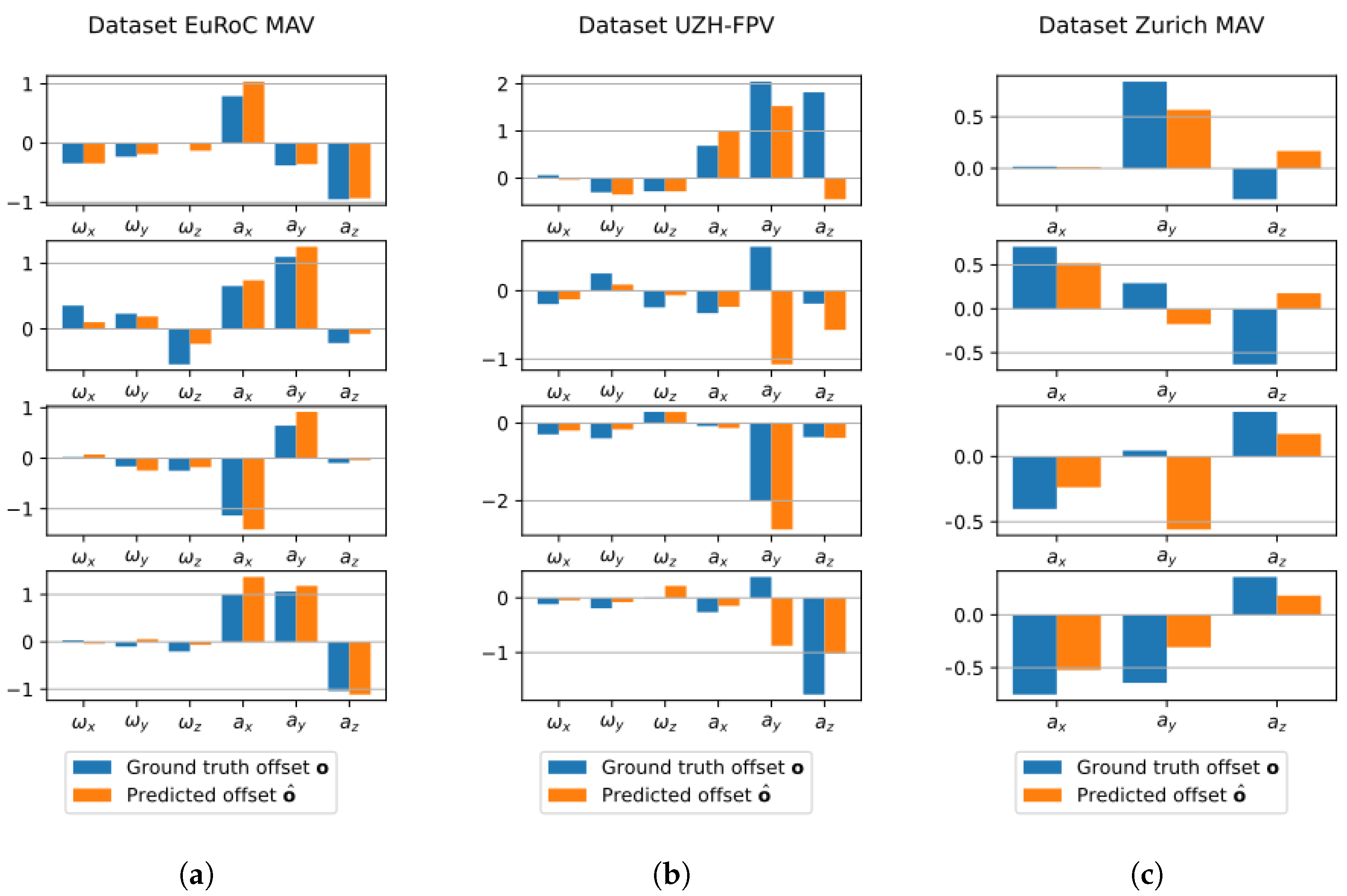
4.3. Results and Discussion
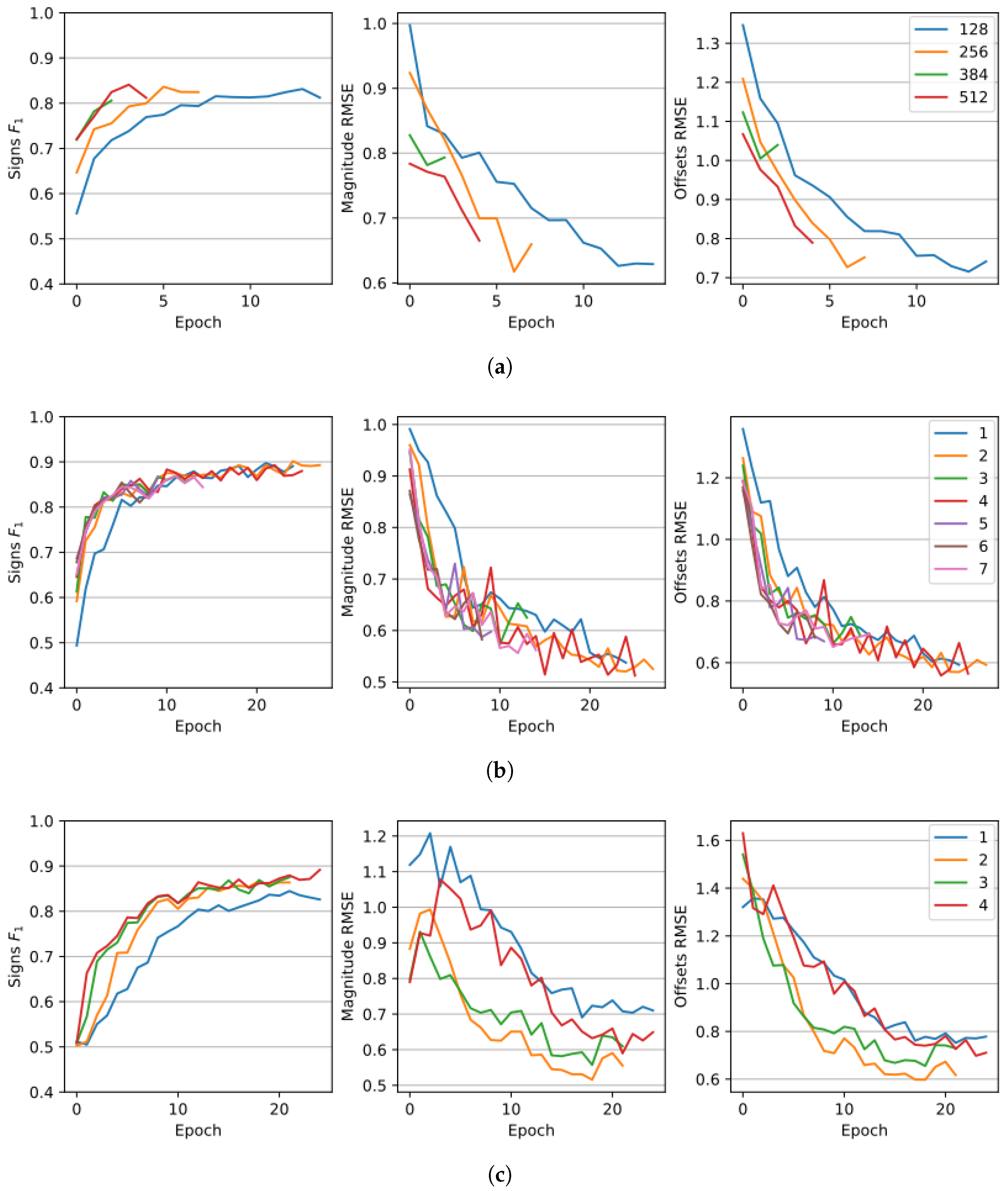
A trial is a syntactic sugar word that consists of a full training and validation procedure. Two kinds of validation schemes [66] have been adopted for the experiments. The k-fold cross-validation scheme has been used in the trials on the Zurich MAV dataset since it is composed of a single video/experiment. In this scheme, windows/samples are partitioned into k groups called folds. To this aim, k different trials are performed using a different fold each time as the validation set and the rest as the training set, averaging the results between each training. The Leave-One-Out (LOO) cross-validation schema, used in UZH-FPV and EuRoC MAV, is a particular case of k-fold cross-validation. In this context, for each trial, the validation fold is each time made of samples from a single video/experiment and the rest of the dataset as the training set. The total number of trials reported is 49:11 for EuRoC MAV, 28 for UZH-FPV, and 10 for Zurich MAV. In the tables, it is worth pointing out that the most relevant parameter is the offset since it represents the overall displacement between the IMU’s measurements and the real values in a real context scenario. The chosen size for the windows/samples is 10 s since, as shown in Table 1, longer sizes yield better results. Increasing the dimension of data provided to the architecture could probably allow for extracting more meaningful information from each sample. However, going too far with the windows’ size could negatively impact the results since it will reduce the number of available samples. At the same time, it will also significantly increase the amount of memory required for training, limiting the proposal’s applicability.
The final configuration of the model has been inferred from the results of the ablation study (Section 4.4) and is the same for each trial and dataset. Table 2 presents a complete overview of the parameters. It is worth noticing that some parameters described in the table are not optimal according to the ablation study in Section 4.4, such as the number of attention heads and the size of the patches. The presented configuration is the one providing the best trade-off between regression and classification performance, as well as computation speed. The following lines describe in more detail the most meaningful ones. The dropout amount has been set to 1 % since it has been empirically found that bigger dropouts are one of the major causes of performance drops among the model’s parameters. The hidden size (referred to as d in Section 3) has been set to 256 since it provides the best tradeoff between the F 1 on signs prediction and the RMSE on magnitudes and offsets. The number of encoder and decoder layers in each transformer encoder and decoder has been set to 2, while the attention heads are 8. The noise multiplier n m , as already mentioned in Section 3.4, is the scalar factor used with the standard deviation of the noise distribution to generate the offsets o . It has been empirically set to 2, since it covers reasonable IMU offsets. The size of the patches (referred to as h p × w p in Section 3) has been set to 64 × 64 since it works much better than a size of 32 × 32 and slightly worse than 96 × 96 . This results in a good compromise between the two sizes in terms of performance since bigger sizes require more epochs to converge, as shown in Section 4.4.
The starting learning rate of the optimizer has been set to 10 5 as in other state-of-the-art works, although AdamW is adaptive, and thus this parameter is not so impactful on the final results. Additionally, videos are first resized to a resolution of 320 × 180 pixels; this operation is performed to have a fixed h = 180 and w = 320 , but it also enables stacking multiple videos into batches. The experiment’s timings and the hardware configuration are shown in Table 3.
The model validation results can be seen in Table 4 and graphically in Figure 2, where sample predictions are shown for six samples of each dataset.
It is interesting to notice that the model is more firm when predicting the offsets on samples from EuRoC MAV and Zurich MAV, whose videos are taken in similar scenarios, while it is more uncertain when dealing with samples from UZH-FPV. In fact, the latter is the only dataset that contains both indoor and outdoor environments, as well as different camera angles (forward-facing and 45° downward-facing). Another possible reason may be the lower resolution of the images: 346 × 260 pixels, compared to the 752 × 480 pixels of EuRoC MAV and the 1920 × 1080 pixels of Zurich MAV. Although the proposed strategy re-scales all the frames to 320 × 180 pixels as a pre-processing step, low-quality starting images may hinder the results.

4.4. Ablation Study

The ablation study consisted of a grid search of the optimal value of several hyper-parameters. There were a series of trials on the UZH-FPV dataset where each one is performed using the base configuration of the model, described in Section 4.3 and Table 2, with a single variation of a parameter. LOO and k-fold cross-validation schemes would require training several instances of the same model on different splits of the dataset and averaging the results. However, from a computational point of view, this would be infeasible. Given that, we chose the compromise to keep fixed training and validation sets to only train a single model once for each combination of parameters. The training and the validation sets are, respectively, random 80 % and 20 % of windows in the dataset. This is a common proportion in the related works and is inspired by the Pareto principle [67]. The results of the ablation study are shown in Table 5 and graphically in Figure 3. Each row in Table 5 represents the trial’s results using different values from the base configuration for specific parameters. An early stopping mechanism has been implemented to stop a trial whenever the training loss does not improve for three consecutive epochs. The metrics used are the same as Section 4.3: the F 1 on signs and RMSE on offsets and magnitudes. The parameters that have been tested are the amount of dropout, the hidden size d, the number of attention heads in the MHA, the number of encoders or decoders in each transformer encoder and transformer decoder, the multiplier for the noise added to o , and the dimension of the patches in the VRB h p × w p .
One of the most impactful parameters is the amount of dropout, which yields a drop of 0.236 in the RMSE offsets considering a dropout of 1 % or 20 % . As can be noticed from the table, for this kind of task, increasing the percentage of dropped connections highly worsens the results. A smaller hidden size d reduces the overfitting but considerably stretches the training time, as can be seen in Figure 3. A hidden size equal to 512, which corresponds to the highest one tested, performs 1.54 % better on the F 1 of the signs with respect to a hidden size of 256. However, the latter value improves the RMSE of offsets and magnitude, respectively, by 0.021 and 0.008 points. Models with 4 and 8 attention heads have been tested. The lowest value outperforms the other by 1.05 % on the F 1 of the signs and nearly 0.02 on the RMSE of offsets and magnitude. Having more attention heads also implies a higher computation demand. However, as it happens for the hidden size and number of layers parameters, a higher number of attention heads lead to a decrease in convergence time. Increasing the number of layers also decreases the convergence time as for Figure 3. On average, the improvement of a model with 4 layers is 0.067 on the RMSE of the offsets and 0.051 on the RMSE of the magnitudes. Considering the F 1 on the signs, 4 is not the best value. However, on average, it improves by 2.32 % , and it is only 0.13 % worse than the best result achieved by a model with 2 layers. A higher noise multiplier n m hinders the capability of the model to accurately distinguish between real signal and noise, as shown in Figure 3. The model performs slightly better on the two RMSEs if the multiplier is set to × 2 since these values represent more plausible noises. Since the estimation of the sign is a binary classification task, it seems that increasing n m helps distinguish the two classes. In fact, the gap between a n m of × 4 and × 1 is 7.69 percentage points on the F 1 signs metric. The size of the patches, inversely proportional to the number of tokens in the first transformer encoder in the VRB, seems to perform better if set with higher values, as can be seen in Figure 3. The worst performing size resulted in 32 × 32 , which is 16.88 % worse on the F 1 signs with respect to a size of 96 × 96 , 0.43 worse on the RMSE offsets and 0.222 worse on the RMSE magnitude. Anyway, higher patches severely mine the computational times and memory requirements. For this reason, we chose the 64 × 64 since it would make a good compromise for a real application on a drone.

5. Conclusions

This work presents a novel neural network architecture for camera-based IMU calibration for UAVs. These procedures are crucial in contexts where the UAV navigation could be only based on a predetermined trajectory to reach the final destination (e.g., in war fields where the GPS signals are usually hijacked) and, in particular, when the route to cover is long. The contribution of this proposal is three-fold. In the first place, it does not make any use of special equipment or impractical hardware procedures to correct the offsets in the sensors, as it could be necessary for other kinds of calibration strategies. In the second place, the proposed pre-trained model can be used directly on the UAV, making it available in a wider range of scenarios. In third place, the algorithm is compatible with both grayscale and RGB images, accommodating different cameras mounted or integrated into diverse UAV models. Moreover, it does not require normalizing the IMU measurements in input, minimizing the computational efforts. More in detail, the algorithm is a transformer-based neural network that processes both a window of sequential frames recorded from the on-board camera and the IMU measurements to estimate the eventual offsets of the latter. The model comprises three modules called video reducer block, IMU reducer block, and noise predictor block. The first two reduce the video and the sequence of the IMU measurements to sequences of tokens of the same shape. These are then summed and given to the latter block to make the final offsets prediction. The approach has been tested on three datasets that are commonly used in the literature for other tasks. Two of them (EuRoC MAV, UZH-FPV) have low-resolution, grayscale-only videos, while the other (Zurich MAV) has full-HD RGB images. Interestingly, the method does not behave much differently on grayscale or RGB images, making it almost camera-agnostic. As expected, the uncertainties are fewer in the two more static datasets and slightly higher in UZH-FPV, which features different environments and camera angles.
One of the issues lies in the fact that the token mixing parts of the transformer encoders and decoders are based on the standard attention mechanism, in which complexity scales quadratically with the number of inputs (e.g., the number of frames of the video and the number of patches in each image). Although this strategy can be considered the standard in transformer-based works, we plan to replace the token, mixing parts with attention-free mechanisms to alleviate the time and space requirements of the neural network. It is worth reminding that, since the offsets are usually small, an IMU calibration has a tangible impact mostly for long traversals. For this reason, one effective way to evaluate the proposed approach would be to analyze data collected from a UAV flying along a straight path for a considerable distance (e.g., 1 Km) and compare the displacement between the predicted and actual final positions. However, to the best of our knowledge, no existing dataset contains data from UAV flights that meet these criteria. We plan to validate the proposed procedure in real-flight test scenarios, in which it is required that the UAV follows a predetermined trajectory toward a destination.

Author Contributions

Conceptualization, D.A., R.L., M.R.M. and A.M.; methodology, D.A., L.C., G.L.F., R.L., M.R.M., A.M. and F.S.; software R.L., M.R.M. and A.M.; validation L.C., G.L.F. and F.S.; writing—original draft preparation, R.L., M.R.M. and A.M.; writing—review and editing, D.A., L.C., G.L.F. and F.S. All authors have read and agreed to the published version of the manuscript.

Funding

This research received no external funding.

Institutional Review Board Statement

Not applicable.

Informed Consent Statement

Not applicable.

Data Availability Statement

Not applicable.

Acknowledgments

This work was supported by the MIUR under grant “Departments of Excellence 2018–2022” of the Department of Computer Science of Sapienza University, the “Smart unmannEd AeRial vehiCles for Human likE monitoRing (SEARCHER)” project of the Italian Ministry of Defence (CIG: Z84333EA0D), the Departmental Strategic Plan (DSP) of the University of Udine—Interdepartmental Project on Artificial Intelligence (2020-25), the ERC Starting Grant no. 802554 (SPECGEO), and the PNRR project FAIR—Future AI Research (PE00000013) under the NRRP MUR program funded by NextGenerationEU.

Conflicts of Interest

The authors declare no conflict of interest.

Abbreviations

The following abbreviations are used in this manuscript:
LOOLeave One Out validation
UAVUnmanned Aerial Vehicle
MAVMicro Aerial Vehicle
LIDARLight Detection And Ranging
FPVFirst Person View
GPSGlobal Positioning System
RGBRed, Green, and Blue channels
HDHigh Definition
IMUInertial Measurement Unit
TPTrue Positive
FPFalse Positive
FNFalse Negative
MSEMean Squared Error
RMSERoot Mean Squared Error
FFNFeed-Forward Network
CNNConvolutional Neural Network
MHAMulti-Head Attention
TETransformer Encoder
TDTransformer Decoder
VRBVideo Reducer Block
IRBIMU Reducer Block
NPBNoise Predictor Block

References

  1. Bonin-Font, F.; Ortiz, A.; Oliver, G. Visual Navigation for Mobile Robots: A Survey. J. Intell. Robot. Syst. 2008, 53, 263. [Google Scholar] [CrossRef]
  2. Yeong, D.J.; Velasco-Hernandez, G.; Barry, J.; Walsh, J. Sensor and Sensor Fusion Technology in Autonomous Vehicles: A Review. Sensors 2021, 21, 2140. [Google Scholar] [CrossRef] [PubMed]
  3. de Ponte Müller, F. Survey on Ranging Sensors and Cooperative Techniques for Relative Positioning of Vehicles. Sensors 2017, 17, 271. [Google Scholar] [CrossRef] [PubMed] [Green Version]
  4. Wu, Y.; Ta, X.; Xiao, R.; Wei, Y.; An, D.; Li, D. Survey of underwater robot positioning navigation. Appl. Ocean. Res. 2019, 90, 101845. [Google Scholar] [CrossRef]
  5. Tariq, Z.B.; Cheema, D.M.; Kamran, M.Z.; Naqvi, I.H. Non-GPS Positioning Systems: A Survey. ACM Comput. Surv. 2017, 50, 1–34. [Google Scholar] [CrossRef]
  6. Bajaj, R.; Ranaweera, S.; Agrawal, D. GPS: Location-tracking technology. Computer 2002, 35, 92–94. [Google Scholar] [CrossRef]
  7. Yuan, Q.; Chen, I.M. Localization and velocity tracking of human via 3 IMU sensors. Sens. Actuators A Phys. 2014, 212, 25–33. [Google Scholar] [CrossRef]
  8. Marsico, M.D.; Mecca, A. Biometric walk recognizer. Multimed. Tools Appl. 2017, 76, 4713–4745. [Google Scholar] [CrossRef] [Green Version]
  9. Steven Eyobu, O.; Han, D. Feature Representation and Data Augmentation for Human Activity Classification Based on Wearable IMU Sensor Data Using a Deep LSTM Neural Network. Sensors 2018, 18, 2892. [Google Scholar] [CrossRef] [Green Version]
  10. Avola, D.; Cinque, L.; Del Bimbo, A.; Marini, M.R. MIFTel: A multimodal interactive framework based on temporal logic rules. Multimed. Tools Appl. 2020, 79, 13533–13558. [Google Scholar] [CrossRef] [Green Version]
  11. Avola, D.; Cinque, L.; Fagioli, A.; Foresti, G.L.; Pannone, D.; Piciarelli, C. Automatic estimation of optimal UAV flight parameters for real-time wide areas monitoring. Multimed. Tools Appl. 2021, 80, 25009–25031. [Google Scholar] [CrossRef]
  12. Avola, D.; Cinque, L.; Foresti, G.L.; Martinel, N.; Pannone, D.; Piciarelli, C. A UAV Video Dataset for Mosaicking and Change Detection from Low-Altitude Flights. IEEE Trans. Syst. Man Cybern. Syst. 2020, 50, 2139–2149. [Google Scholar] [CrossRef] [Green Version]
  13. Conforti, M.; Mercuri, M.; Borrelli, L. Morphological changes detection of a large earthflow using archived images, lidar-derived dtm, and uav-based remote sensing. Remote Sens. 2020, 13, 120. [Google Scholar] [CrossRef]
  14. Avola, D.; Cannistraci, I.; Cascio, M.; Cinque, L.; Diko, A.; Fagioli, A.; Foresti, G.L.; Lanzino, R.; Mancini, M.; Mecca, A.; et al. A Novel GAN-Based Anomaly Detection and Localization Method for Aerial Video Surveillance at Low Altitude. Remote Sens. 2022, 14, 4110. [Google Scholar] [CrossRef]
  15. Hamdi, S.; Bouindour, S.; Snoussi, H.; Wang, T.; Abid, M. End-to-end deep one-class learning for anomaly detection in uav video stream. J. Imaging 2021, 7, 90. [Google Scholar] [CrossRef] [PubMed]
  16. Avola, D.; Cinque, L.; Di Mambro, A.; Diko, A.; Fagioli, A.; Foresti, G.L.; Marini, M.R.; Mecca, A.; Pannone, D. Low-Altitude Aerial Video Surveillance via One-Class SVM Anomaly Detection from Textural Features in UAV Images. Information 2022, 13, 2. [Google Scholar] [CrossRef]
  17. Avola, D.; Cinque, L.; Diko, A.; Fagioli, A.; Foresti, G.L.; Mecca, A.; Pannone, D.; Piciarelli, C. MS-Faster R-CNN: Multi-Stream Backbone for Improved Faster R-CNN Object Detection and Aerial Tracking from UAV Images. Remote Sens. 2021, 13, 1670. [Google Scholar] [CrossRef]
  18. Örnhag, M.V.; Persson, P.; Wadenbäck, M.; Åström, K.; Heyden, A. Trust Your IMU: Consequences of Ignoring the IMU Drift. In Proceedings of the IEEE/CVF Conference on Computer Vision and Pattern Recognition (CVPR) Workshops, New Orleans, LA, USA, 19–20 June 2022; pp. 4468–4477. [Google Scholar] [CrossRef]
  19. Couturier, A.; Akhloufi, M.A. A review on absolute visual localization for UAV. Robot. Auton. Syst. 2021, 135, 103666. [Google Scholar] [CrossRef]
  20. Munaye, Y.Y.; Lin, H.P.; Adege, A.B.; Tarekegn, G.B. UAV Positioning for Throughput Maximization Using Deep Learning Approaches. Sensors 2019, 19, 2775. [Google Scholar] [CrossRef] [Green Version]
  21. Vaswani, A.; Shazeer, N.; Parmar, N.; Uszkoreit, J.; Jones, L.; Gomez, A.N.; Kaiser, L.; Polosukhin, I. Attention is All You Need. In Proceedings of the 31st International Conference on Neural Information Processing Systems, NIPS’17, Long Beach, CA, USA, 4–9 December 2017; Curran Associates Inc.: Red Hook, NY, USA, 2017; pp. 6000–6010. [Google Scholar] [CrossRef]
  22. Devlin, J.; Chang, M.W.; Lee, K.; Toutanova, K. BERT: Pre-training of Deep Bidirectional Transformers for Language Understanding. In Proceedings of the 2019 Conference of the North American Chapter of the Association for Computational Linguistics: Human Language Technologies, Minneapolis, MN, USA, 2–7 June 2019; Volume 1 (Long and Short Papers), pp. 4171–4186. [Google Scholar] [CrossRef]
  23. Zaheer, M.; Guruganesh, G.; Dubey, K.A.; Ainslie, J.; Alberti, C.; Ontanon, S.; Pham, P.; Ravula, A.; Wang, Q.; Yang, L.; et al. Big Bird: Transformers for Longer Sequences. Adv. Neural Inf. Process. Syst. 2020, 33, 17283–17297. [Google Scholar] [CrossRef]
  24. Brown, T.; Mann, B.; Ryder, N.; Subbiah, M.; Kaplan, J.D.; Dhariwal, P.; Neelakantan, A.; Shyam, P.; Sastry, G.; Askell, A.; et al. Language Models are Few-Shot Learners. Adv. Neural Inf. Process. Syst. 2020, 33, 1877–1901. [Google Scholar] [CrossRef]
  25. Liu, Z.; Lin, Y.; Cao, Y.; Hu, H.; Wei, Y.; Zhang, Z.; Lin, S.; Guo, B. Swin Transformer: Hierarchical Vision Transformer Using Shifted Windows. In Proceedings of the 2021 IEEE/CVF International Conference on Computer Vision (ICCV), Montreal, BC, Canada, 10–17 October 2021; pp. 9992–10002. [Google Scholar] [CrossRef]
  26. Zhang, Y.; Li, X.; Liu, C.; Shuai, B.; Zhu, Y.; Brattoli, B.; Chen, H.; Marsic, I.; Tighe, J. VidTr: Video Transformer without Convolutions. In Proceedings of the 2021 IEEE/CVF International Conference on Computer Vision (ICCV), Montreal, BC, Canada, 10–17 October 2021; pp. 13557–13567. [Google Scholar] [CrossRef]
  27. Kolesnikov, A.; Dosovitskiy, A.; Weissenborn, D.; Heigold, G.; Uszkoreit, J.; Beyer, L.; Minderer, M.; Dehghani, M.; Houlsby, N.; Gelly, S.; et al. An Image Is Worth 16 × 16 Words: Transformers for Image Recognition at Scale. arXiv 2010, arXiv:2010.11929. [Google Scholar]
  28. Baevski, A.; Zhou, Y.; Mohamed, A.; Auli, M. wav2vec 2.0: A Framework for Self-Supervised Learning of Speech Representations. In Proceedings of the Advances in Neural Information Processing Systems, Online, 6–12 December 2020; Larochelle, H., Ranzato, M., Hadsell, R., Balcan, M., Lin, H., Eds.; Association for Computing Machinery: New York, NY, USA, 2020; Volume 33, pp. 12449–12460. [Google Scholar] [CrossRef]
  29. Xing, D.; Evangeliou, N.; Tsoukalas, A.; Tzes, A. Siamese Transformer Pyramid Networks for Real-Time UAV Tracking. In Proceedings of the 2022 IEEE/CVF Winter Conference on Applications of Computer Vision (WACV), Waikoloa, HI, USA, 3–6 July 2022; pp. 1898–1907. [Google Scholar] [CrossRef]
  30. Ye, J.; Fu, C.; Cao, Z.; An, S.; Zheng, G.; Li, B. Tracker Meets Night: A Transformer Enhancer for UAV Tracking. IEEE Robot. Autom. Lett. 2022, 7, 3866–3873. [Google Scholar] [CrossRef]
  31. Ghali, R.; Akhloufi, M.A.; Mseddi, W.S. Deep Learning and Transformer Approaches for UAV-Based Wildfire Detection and Segmentation. Sensors 2022, 22, 1977. [Google Scholar] [CrossRef] [PubMed]
  32. Parcollet, T.; Ravanelli, M. The Energy and Carbon Footprint of Training End-to-End Speech Recognizers. 2021. Available online: https://hal.science/hal-03190119/ (accessed on 22 December 2022).
  33. Xiao, Y.; Ruan, X.; Chai, J.; Zhang, X.; Zhu, X. Online IMU Self-Calibration for Visual-Inertial Systems. Sensors 2019, 19, 1624. [Google Scholar] [CrossRef] [Green Version]
  34. Henawy, J.; Li, Z.; Yau, W.Y.; Seet, G. Accurate IMU Factor Using Switched Linear Systems for VIO. IEEE Trans. Ind. Electron. 2021, 68, 7199–7208. [Google Scholar] [CrossRef]
  35. Qin, T.; Li, P.; Shen, S. VINS-Mono: A Robust and Versatile Monocular Visual-Inertial State Estimator. IEEE Trans. Robot. 2018, 34, 1004–1020. [Google Scholar] [CrossRef] [Green Version]
  36. Carlevaris-Bianco, N.; Ushani, A.K.; Eustice, R.M. University of Michigan North Campus long-term vision and lidar dataset. Int. J. Robot. Res. 2016, 35, 1023–1035. [Google Scholar] [CrossRef]
  37. Burri, M.; Nikolic, J.; Gohl, P.; Schneider, T.; Rehder, J.; Omari, S.; Achtelik, M.W.; Siegwart, R. The EuRoC micro aerial vehicle datasets. Int. J. Robot. Res. 2016, 35, 1157–1163. [Google Scholar] [CrossRef]
  38. Pfrommer, B.; Sanket, N.; Daniilidis, K.; Cleveland, J. PennCOSYVIO: A challenging Visual Inertial Odometry benchmark. In Proceedings of the 2017 IEEE International Conference on Robotics and Automation (ICRA), Singapore, 29 May–3 June 2017; pp. 3847–3854. [Google Scholar] [CrossRef]
  39. Majdik, A.L.; Till, C.; Scaramuzza, D. The Zurich urban micro aerial vehicle dataset. Int. J. Robot. Res. 2017, 36, 269–273. [Google Scholar] [CrossRef] [Green Version]
  40. Schubert, D.; Goll, T.; Demmel, N.; Usenko, V.; Stückler, J.; Cremers, D. The TUM VI Benchmark for Evaluating Visual-Inertial Odometry. In Proceedings of the 2018 IEEE/RSJ International Conference on Intelligent Robots and Systems (IROS), Madrid, Spain, 1–5 October 2018; pp. 1680–1687. [Google Scholar] [CrossRef] [Green Version]
  41. Qiu, D.; Li, S.; Wang, T.; Ye, Q.; Li, R.; Ding, K.; Xu, H. A high-precision calibration approach for Camera-IMU pose parameters with adaptive constraints of multiple error equations. Measurement 2020, 153, 107402. [Google Scholar] [CrossRef]
  42. Lee, Y.; Yoon, J.; Yang, H.; Kim, C.; Lee, D. Camera-GPS-IMU sensor fusion for autonomous flying. In Proceedings of the 2016 Eighth International Conference on Ubiquitous and Future Networks (ICUFN), Vienna, Austria, 5–8 July 2016; pp. 85–88. [Google Scholar] [CrossRef]
  43. Ren, C.; Liu, Q.; Fu, T. A Novel Self-Calibration Method for MIMU. IEEE Sens. J. 2015, 15, 5416–5422. [Google Scholar] [CrossRef]
  44. Hausman, K.; Weiss, S.; Brockers, R.; Matthies, L.; Sukhatme, G.S. Self-calibrating multi-sensor fusion with probabilistic measurement validation for seamless sensor switching on a UAV. In Proceedings of the 2016 IEEE International Conference on Robotics and Automation (ICRA), Stockholm, Sweden, 16–21 May 2016; pp. 4289–4296. [Google Scholar] [CrossRef]
  45. Huang, B.; Feng, P.; Zhang, J.; Yu, D.; Wu, Z. A Novel Positioning Module and Fusion Algorithm for Unmanned Aerial Vehicle Monitoring. IEEE Sens. J. 2021, 21, 23006–23023. [Google Scholar] [CrossRef]
  46. Sanjukumar, N.; Koundinya, P.N.; Rajalakshmi, P. Novel technique for Multi Sensor Calibration of a UAV. In Proceedings of the 2020 IEEE International Conference on Computing, Power and Communication Technologies (GUCON), Greater Noida, India, 2–4 October 2020; pp. 778–782. [Google Scholar] [CrossRef]
  47. Li, M.; Yu, H.; Zheng, X.; Mourikis, A.I. High-fidelity sensor modeling and self-calibration in vision-aided inertial navigation. In Proceedings of the 2014 IEEE International Conference on Robotics and Automation (ICRA), Hong Kong, China, 31 May–5 June 2014; pp. 409–416. [Google Scholar] [CrossRef] [Green Version]
  48. Hwangbo, M.; Kim, J.S.; Kanade, T. IMU Self-Calibration Using Factorization. IEEE Trans. Robot. 2013, 29, 493–507. [Google Scholar] [CrossRef] [Green Version]
  49. Wu, Y.; Goodall, C.; El-Sheimy, N. Self-calibration for IMU/odometer land navigation: Simulation and test results. In Proceedings of the 2010 International Technical Meeting of The Institute of Navigation, Portland, OR, USA, 21–24 September 2010; pp. 839–849. [Google Scholar]
  50. Yang, Y.; Geneva, P.; Zuo, X.; Huang, G. Online Self-Calibration for Visual-Inertial Navigation Systems: Models, Analysis and Degeneracy. arXiv 2022, arXiv:2201.09170. [Google Scholar]
  51. Huang, F.; Wang, Z.; Xing, L.; Gao, C. A MEMS IMU Gyroscope Calibration Method Based on Deep Learning. IEEE Trans. Instrum. Meas. 2022, 71, 1–9. [Google Scholar] [CrossRef]
  52. Mahdi, A.E.; Azouz, A.; Abdalla, A.; Abosekeen, A. IMU-Error Estimation and Cancellation Using ANFIS for Improved UAV Navigation. In Proceedings of the 2022 13th International Conference on Electrical Engineering (ICEENG), Cairo, Egypt, 29–31 March 2022; pp. 120–124. [Google Scholar] [CrossRef]
  53. Buchanan, R.; Agrawal, V.; Camurri, M.; Dellaert, F.; Fallon, M. Deep IMU Bias Inference for Robust Visual-Inertial Odometry with Factor Graphs. IEEE Robot. Autom. Lett. 2023, 8, 41–48. [Google Scholar] [CrossRef]
  54. Hochreiter, S.; Schmidhuber, J. Long Short-Term Memory. Neural Comput. 1997, 9, 1735–1780. [Google Scholar] [CrossRef]
  55. Steinbrener, J.; Brommer, C.; Jantos, T.; Fornasier, A.; Weiss, S. Improved State Propagation through AI-based Pre-processing and Down-sampling of High-Speed Inertial Data. In Proceedings of the 2022 International Conference on Robotics and Automation (ICRA), Philadelphia, PA, USA, 23–27 May 2022; pp. 6084–6090. [Google Scholar] [CrossRef]
  56. Ioffe, S.; Szegedy, C. Batch Normalization: Accelerating Deep Network Training by Reducing Internal Covariate Shift. In Proceedings of the 32nd International Conference on International Conference on Machine Learning, Lille, France, 6–11 July 2015; Volume 37, pp. 448–456. [Google Scholar] [CrossRef]
  57. He, K.; Zhang, X.; Ren, S.; Sun, J. Deep Residual Learning for Image Recognition. In Proceedings of the 2016 IEEE Conference on Computer Vision and Pattern Recognition (CVPR), Las Vegas, NV, USA, 27–30 June 2016; pp. 770–778. [Google Scholar] [CrossRef] [Green Version]
  58. Hinton, G.E.; Srivastava, N.; Krizhevsky, A.; Sutskever, I.; Salakhutdinov, R.R. Improving neural networks by preventing co-adaptation of feature detectors. arXiv 2012, arXiv:1207.0580. [Google Scholar]
  59. Ba, J.L.; Kiros, J.R.; Hinton, G.E. Layer Normalization. arXiv 2016, arXiv:1607.06450. [Google Scholar]
  60. Srivastava, R.K.; Greff, K.; Schmidhuber, J. Training Very Deep Networks. Adv. Neural Inf. Process. Syst. 2015, 9, 2377–2385. [Google Scholar]
  61. Shaw, P.; Uszkoreit, J.; Vaswani, A. Self-Attention with Relative Position Representations. In Proceedings of the 2018 Conference of the North American Chapter of the Association for Computational Linguistics: Human Language Technologies, New Orleans, LA, USA, 2–4 June 2018; Volume 2 (Short Papers), pp. 464–468. [Google Scholar] [CrossRef] [Green Version]
  62. Jordan, M.I.; Mitchell, T.M. Machine learning: Trends, perspectives, and prospects. Science 2015, 349, 255–260. [Google Scholar] [CrossRef] [PubMed]
  63. Loshchilov, I.; Hutter, F. Decoupled Weight Decay Regularization. arXiv 2017, arXiv:1711.05101. [Google Scholar]
  64. Kingma, D.P.; Ba, J. Adam: A Method for Stochastic Optimization. In Proceedings of the ICLR (Poster), San Diego, CA, USA, 7–9 May 2015. [Google Scholar]
  65. Delmerico, J.; Cieslewski, T.; Rebecq, H.; Faessler, M.; Scaramuzza, D. Are We Ready for Autonomous Drone Racing? The UZH-FPV Drone Racing Dataset. In Proceedings of the 2019 International Conference on Robotics and Automation (ICRA), Montreal, QC, Canada, 20–24 May 2019; pp. 6713–6719. [Google Scholar] [CrossRef]
  66. Wong, T.T. Performance evaluation of classification algorithms by k-fold and leave-one-out cross validation. Pattern Recognit. 2015, 48, 2839–2846. [Google Scholar] [CrossRef]
  67. Jana, P.; Tiwari, M. 2—Lean terms in apparel manufacturing. In Lean Tools in Apparel Manufacturing; Jana, P., Tiwari, M., Eds.; The Textile Institute Book Series; Woodhead Publishing: Sawston, UK, 2021; pp. 17–45. [Google Scholar] [CrossRef]
Figure 1. The architecture of the model. A dashed line between two modules means weight sharing between them. (a) Overview of the full model. The outputs of the video reducer block (VRB) and of the IMU reducer block (IRB) are summed and passed to the noise predictor block that will output the final offset estimation o ^ R 6 ; (b) (overview of the video reducer block (VRB)). The input frames F R n × h × w are unfolded into patches that are projected into token vectors and processed by two transformer encoder to output a token for each frame T v ( enc ) R n × d ; (c) (overview of the IMU reducer block (IRB)). The input IMU measurements I R n × 6 are projected into a d-dimensional space and then processed by a transformer encoder to output a representation T i ( enc ) R n × d of the measurements; (d) Overview of the noise predictor block (NPB). The tokens T R n × d obtained from the sum of the outputs of the VRB and the IRB are passed through a transformer encoder and its results T ( enc ) R n × d to a transformer decoder along with a query matrix L R 1 × d . The output is the predicted offsets o ^ R 6 .
Sensors 23 02655 g001aSensors 23 02655 g001b
Figure 2. Sample predictions of the model on the datasets. Values ω x , ω y , and ω z are, respectively, the measurement of the gyroscope for the three axes, while a x , a y , and a z are the corresponding ones from the accelerometer. (a) EuRoC MAV [37]; (b) UZH-FPV [65]; (c) Zurich MAV [39].
Sensors 23 02655 g002
Figure 3. Plots of the results of the ablation study on four parameters of the model. (a) Hidden size (d). (b) Number of layers in the encoders and the decoders. (c) Injected noise multiplier ( n m ). (d) Size of the patches ( h p , w p ).
Sensors 23 02655 g003aSensors 23 02655 g003b
Table 1. Results of the experiments at various window sizes. The experiments have been performed on UZH-FPV [65] dataset, the most challenging and various among the ones analyzed in this work. Train and validation sets follow an 80/20% split, fixed between experiments and chosen as described in Section 4.4. The stride of the windows is kept fixed to 1 s alongside the seed. The best value in each result column is in bold.
Window SizeSigns F 1 Offsets RMSE
2 s 87.4%0.686
4 s 87.9%0.616
6 s 87.4%0.532
8 s 90.1%0.563
10 s 91.8%0.495
Table 2. The configuration of the model used in the final evaluations.
ParameterValue
Dropout 1 %
Hidden size (d)256
Attention heads8
Layers2
Noise multiplier ( n m ) 2 ×
Patches size ( h p × w p ) 64 × 64
Batch size 16 dataset is EuRoC MAV or UZH - FPV 8 dataset is Zurich MAV
Activation function ( σ )Rectified Linear Unit: R e L U ( x ) = max ( 0 , x )
Learning rate 10 5
Table 3. Times and stats of the experiments. All the experiments have been run sequentially on a cluster’s node with 64 GB DDR4 RAM memory, 1 × AMD Epyc 7301 2.2 G Hz CPU core, and a Nvidia Quadro 6000 GPU with 24 GB of RAM.
DatasetValidation TypeNumber of TrialsBatch Size
EuRoC MAV [37]LOO1116
UZH-FPV [65]LOO2816
Zurich MAV [39]10-fold108
DatasetEpochs per TrialTime per TrialTime per Every Trial
EuRoC MAV [37]17.5 803.2  s 8835.4  s
UZH-FPV [65]13.6 1136.3  s 31,815.4  s
Zurich MAV [39]4.7 1214.3  s 12,142.9  s
DatasetBatches per Training EpochTime per Training StepTime per Training Epoch
EuRoC MAV [37]69 0.607  s 41.9  s
UZH-FPV [65]133 0.620  s 82.5  s
Zurich MAV [39]300 0.801  s 240.2  s
DatasetBatches per Validation EpochTime per Validation StepTime per Validation Epoch
EuRoC MAV [37]10 0.412  s 4.1  s
UZH-FPV [65]3 0.422  s 1.3  s
Zurich MAV [39]33 0.551  s 18.2  s
Table 4. Results on the three datasets. Each numerical cell is composed of the mean and standard deviation between the best values of each validation split.
DatasetValidationSigns F 1 Magnitude RMSEOffsets RMSE
EuRoC MAV [37]LOO94.59%/1.55%0.177/0.0440.193/0.062
UZH-FPV [65]LOO89.61%/3.57%0.454/0.1640.502/0.203
Zurich MAV [39]10-fold73.79%/3.84%0.273/0.0380.360/0.049
Table 5. Results of the ablation study. Variations of several parameters of the model have been tested, and this table shows the results of the best score on the validation set of each trial. The best value in each result column for a particular parameter is in bold.
ParameterValueSigns F 1 Magnitude RMSEOffsets RMSE
Dropout0%80.62%0.6310.750
Dropout1%80.53%0.6350.749
Dropout5%78.29%0.6620.792
Dropout10%72.30%0.7410.932
Dropout20%70.51%0.7760.986
Hidden size12878.51%0.7200.862
Hidden size25679.67%0.7330.862
Hidden size38479.39%0.7881.022
Hidden size51281.21%0.7280.883
Attention heads479.04%0.6630.793
Attention heads877.99%0.6840.818
Layers183.51%0.6690.780
Layers285.79%0.6100.706
Layers383.82%0.6610.789
Layers485.66%0.6020.699
Layers582.17%0.6670.786
Layers681.55%0.6730.778
Layers783.22%0.6370.755
Noise multiplier 1 × 74.83%0.8790.968
Noise multiplier 2 × 78.49%0.6650.809
Noise multiplier 3 × 80.76%0.6900.839
Noise multiplier 4 × 82.52%0.8000.946
Patches size 32 × 32 59.97%0.9191.276
Patches size 64 × 64 73.89%0.7500.929
Patches size 96 × 96 76.85%0.6970.841
Patches size 128 × 128 72.04%0.7870.976
Disclaimer/Publisher’s Note: The statements, opinions and data contained in all publications are solely those of the individual author(s) and contributor(s) and not of MDPI and/or the editor(s). MDPI and/or the editor(s) disclaim responsibility for any injury to people or property resulting from any ideas, methods, instructions or products referred to in the content.

