Author Contributions
Conceptualization, X.Z. and C.L. (Chao Liu); Methodology, S.Y.; Software, S.Y.; Validation, S.Y. and C.L. (Chunyang Liu); Formal analysis, X.Z. and C.L. (Chao Liu); Investigation, S.Y., C.L. (Chao Liu), J.C. and C.L. (Chunyang Liu); Resources, J.C.; Data curation, S.Y.; Writing—original draft, S.Y.; Writing—review & editing, X.Z.; Visualization, S.Y. and C.L. (Chunyang Liu); Supervision, X.Z., C.L. (Chao Liu) and J.C.; Project administration, X.Z.; Funding acquisition, X.Z. All authors have read and agreed to the published version of the manuscript.
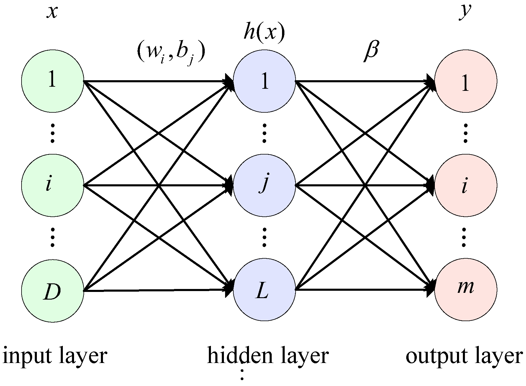
Figure 1.
The architecture of ELM.
Figure 1.
The architecture of ELM.
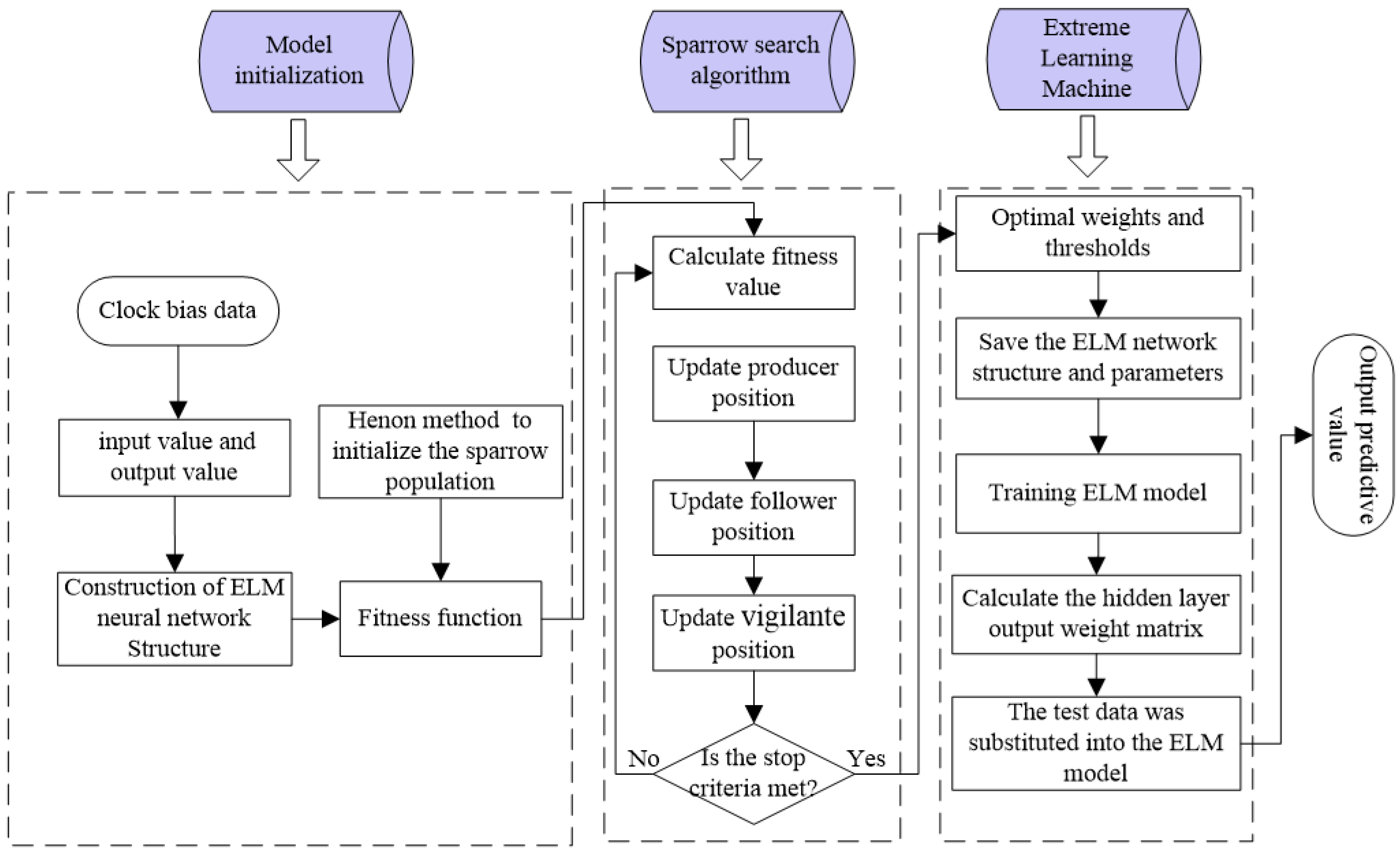
Figure 2.
The workflow of the proposed SSA-ELM algorithm.
Figure 2.
The workflow of the proposed SSA-ELM algorithm.
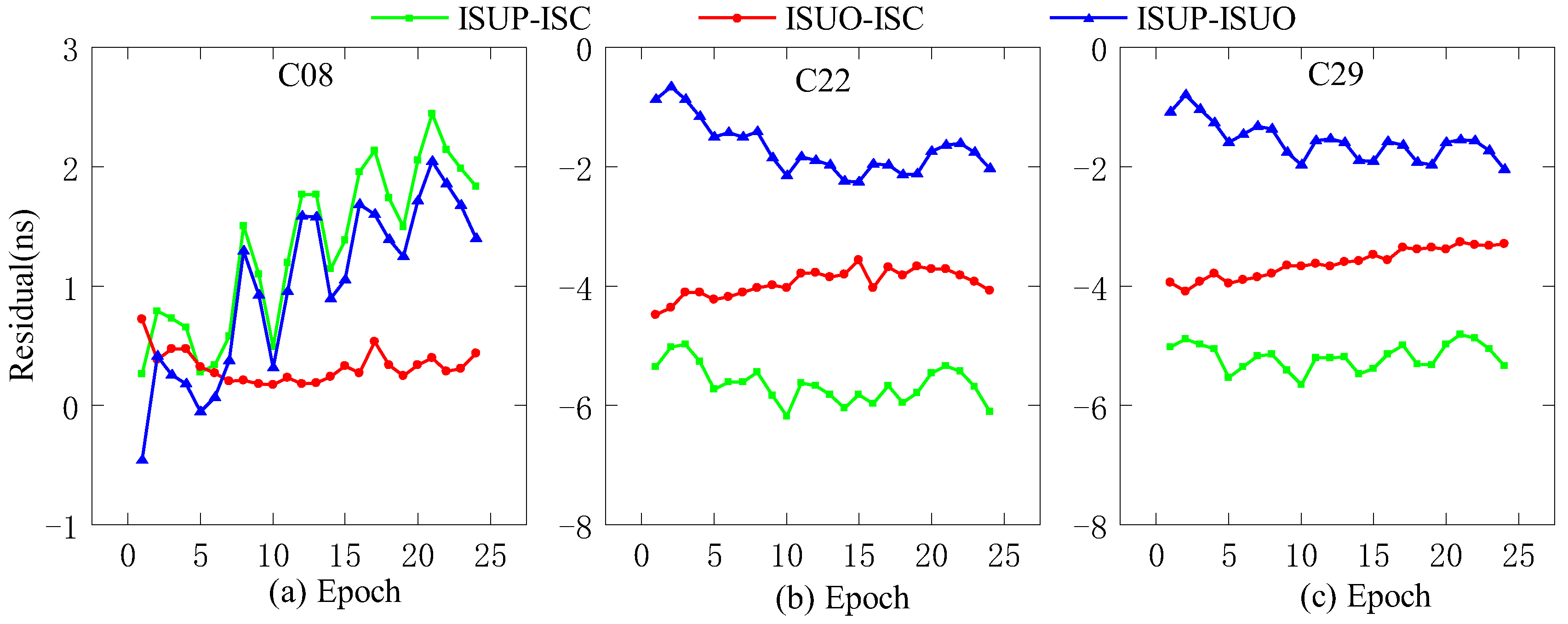
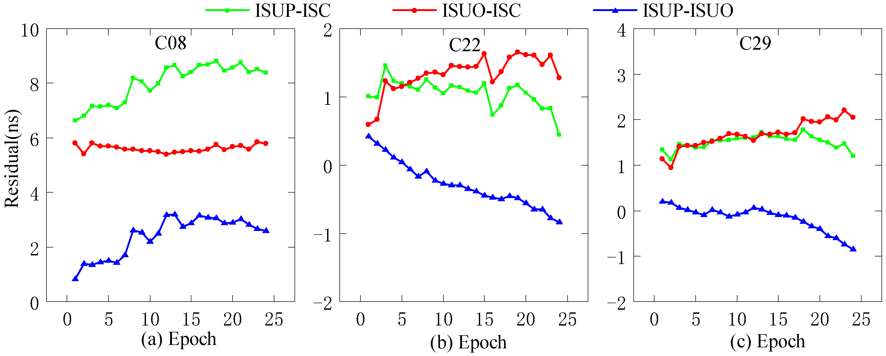
Figure 3.
The residual plot of the RB clock as a reference clock. (a) The residual value of C08 predicted after 6 h. (b) The residual value of C22 predicted after 6 h. (c) The residual value of C29 predicted after 6 h.
Figure 3.
The residual plot of the RB clock as a reference clock. (a) The residual value of C08 predicted after 6 h. (b) The residual value of C22 predicted after 6 h. (c) The residual value of C29 predicted after 6 h.
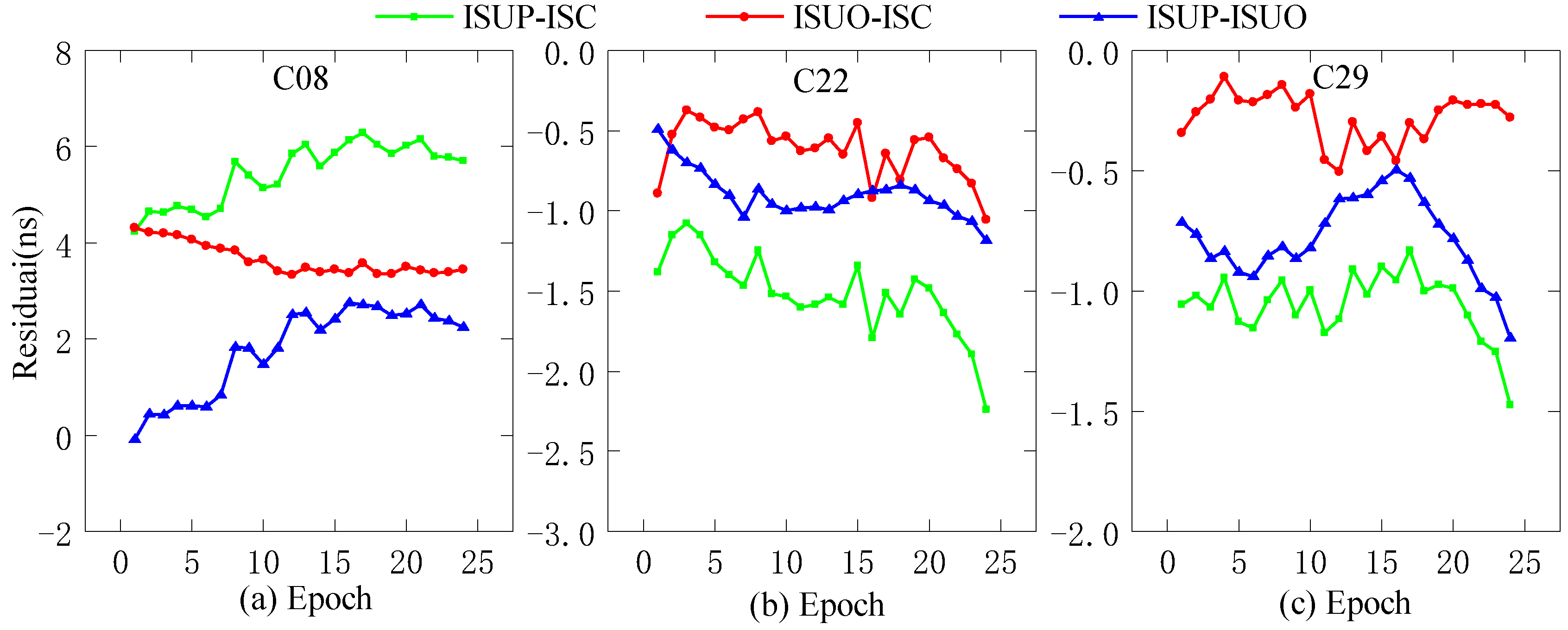
Figure 4.
The residual plot of the Rb-II clock as the reference clock. (a) The residual value of C08 predicted after 6 h. (b) The residual value of C22 predicted after 6 h. (c) The residual value of C29 predicted after 6 h.
Figure 4.
The residual plot of the Rb-II clock as the reference clock. (a) The residual value of C08 predicted after 6 h. (b) The residual value of C22 predicted after 6 h. (c) The residual value of C29 predicted after 6 h.
Figure 5.
The residual plot of the PHM clock as the reference clock. (a) The residual value of C08 predicted after 6 h. (b) The residual value of C22 predicted after 6 h. (c) The residual value of C29 predicted after 6 h.
Figure 5.
The residual plot of the PHM clock as the reference clock. (a) The residual value of C08 predicted after 6 h. (b) The residual value of C22 predicted after 6 h. (c) The residual value of C29 predicted after 6 h.
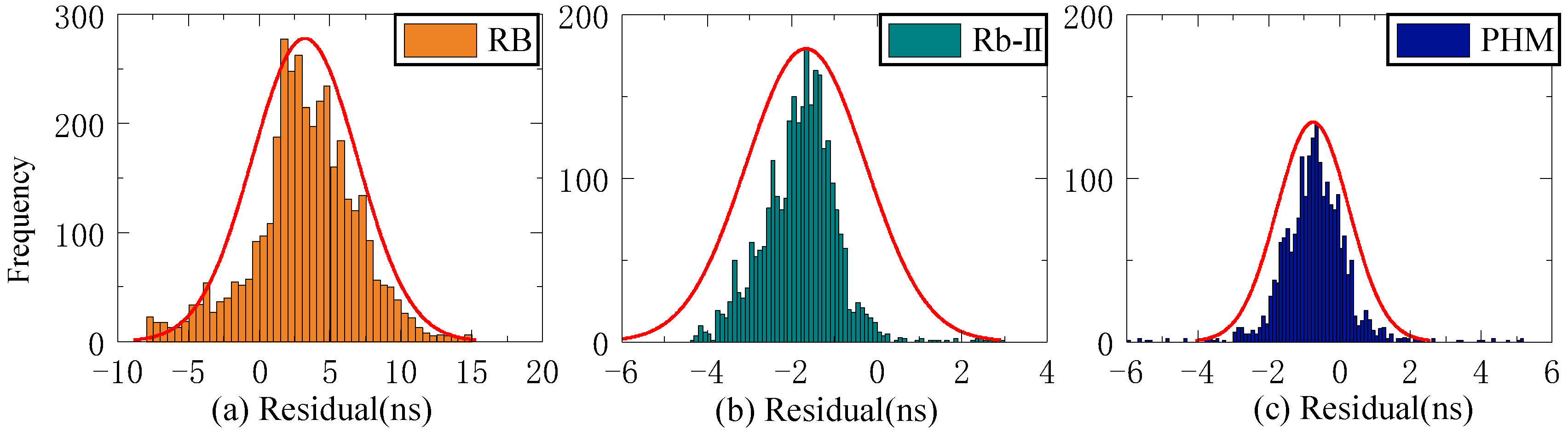
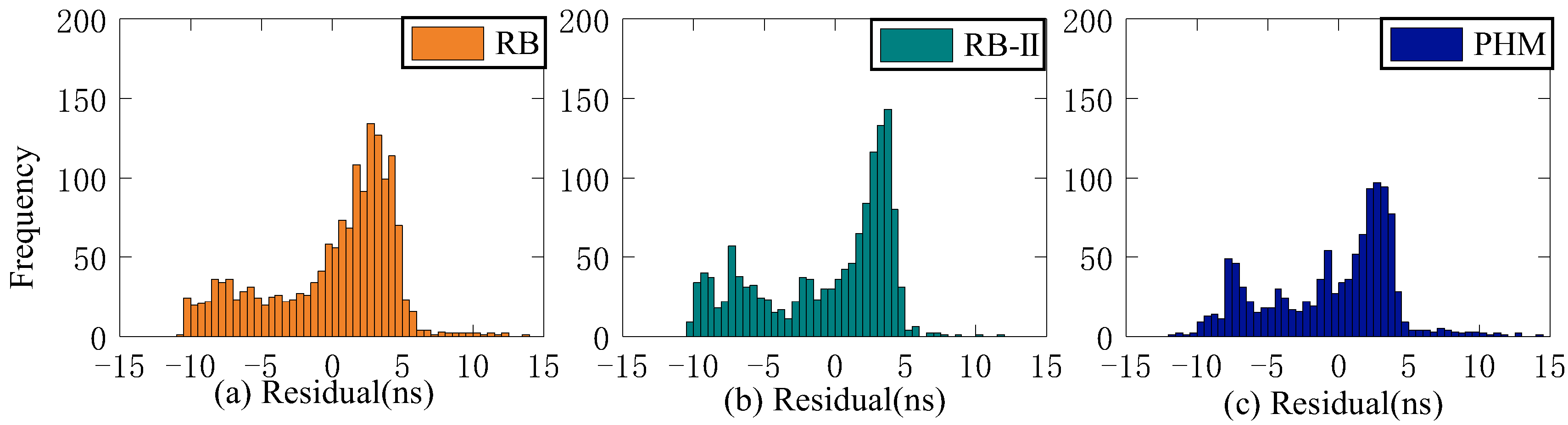
Figure 6.
The ISUP-ISC residuals of three atomic clocks. (a) The residual distribution of the RB clock. (b) The residual distribution of the Rb-II clock. (c) The residual distribution of the PHM clock.
Figure 6.
The ISUP-ISC residuals of three atomic clocks. (a) The residual distribution of the RB clock. (b) The residual distribution of the Rb-II clock. (c) The residual distribution of the PHM clock.
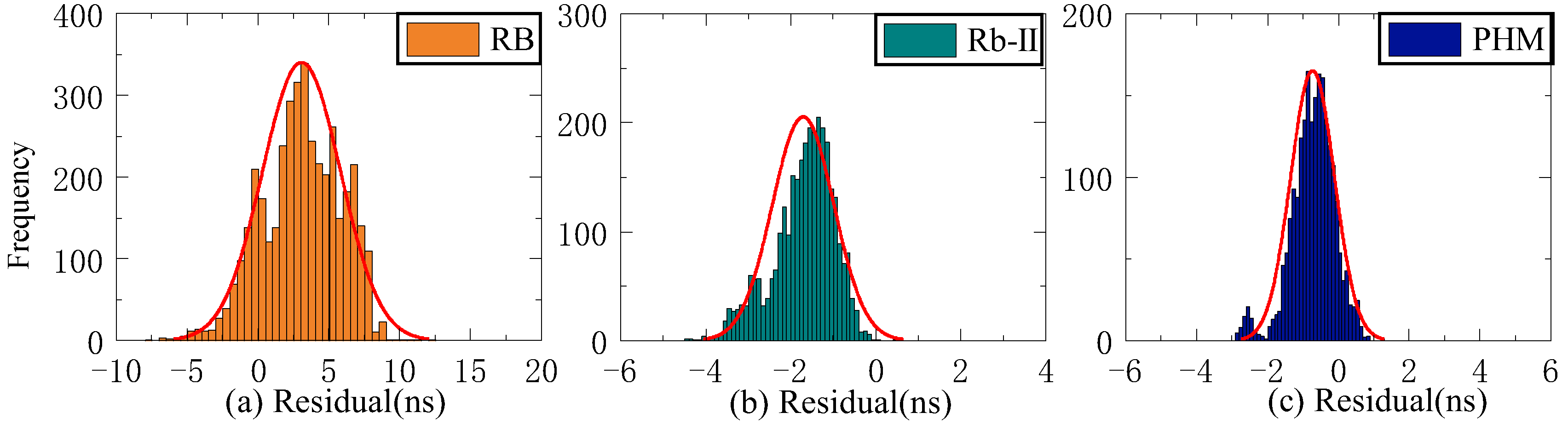
Figure 7.
The ISUO-ISC residuals of three atomic clocks. (a) The residual distribution of the RB clock. (b) The residual distribution of the Rb-II clock. (c) The residual distribution of the PHM clock.
Figure 7.
The ISUO-ISC residuals of three atomic clocks. (a) The residual distribution of the RB clock. (b) The residual distribution of the Rb-II clock. (c) The residual distribution of the PHM clock.
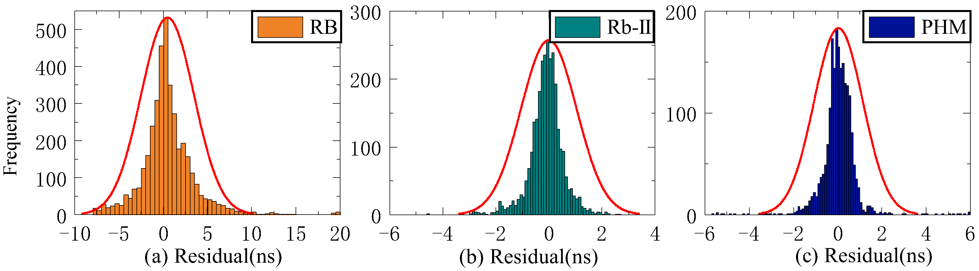
Figure 8.
The ISUP-ISUO residuals of three atomic clocks. (a) The residual distribution of the RB clock. (b) The residual distribution of the Rb-II clock. (c) The residual distribution of the PHM clock.
Figure 8.
The ISUP-ISUO residuals of three atomic clocks. (a) The residual distribution of the RB clock. (b) The residual distribution of the Rb-II clock. (c) The residual distribution of the PHM clock.
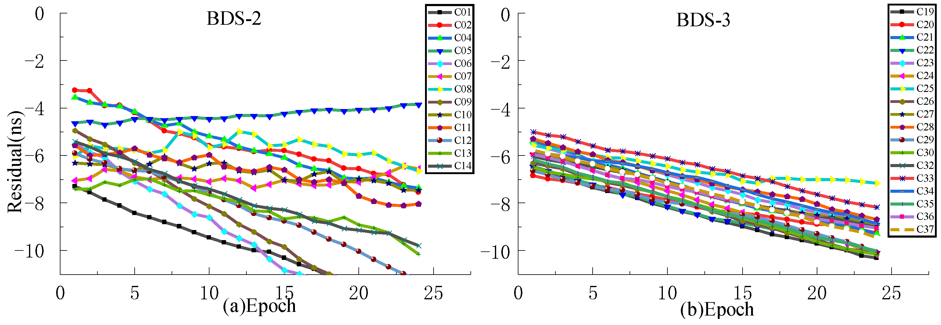
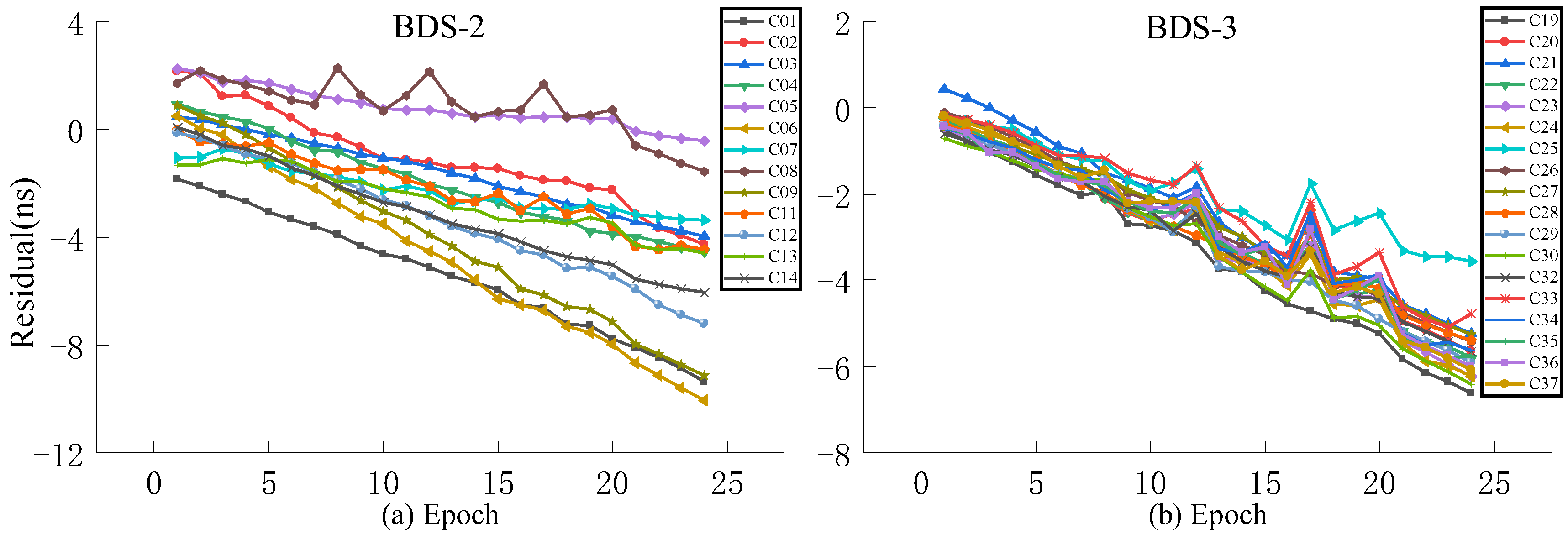
Figure 9.
The residual plot of the ISUP model using the initial hour update ultra-fast clock product of the next day. (a) The residual value of BDS-2 predicted after 6 h. (b) The residual value of BDS-3 predicted after 6 h.
Figure 9.
The residual plot of the ISUP model using the initial hour update ultra-fast clock product of the next day. (a) The residual value of BDS-2 predicted after 6 h. (b) The residual value of BDS-3 predicted after 6 h.
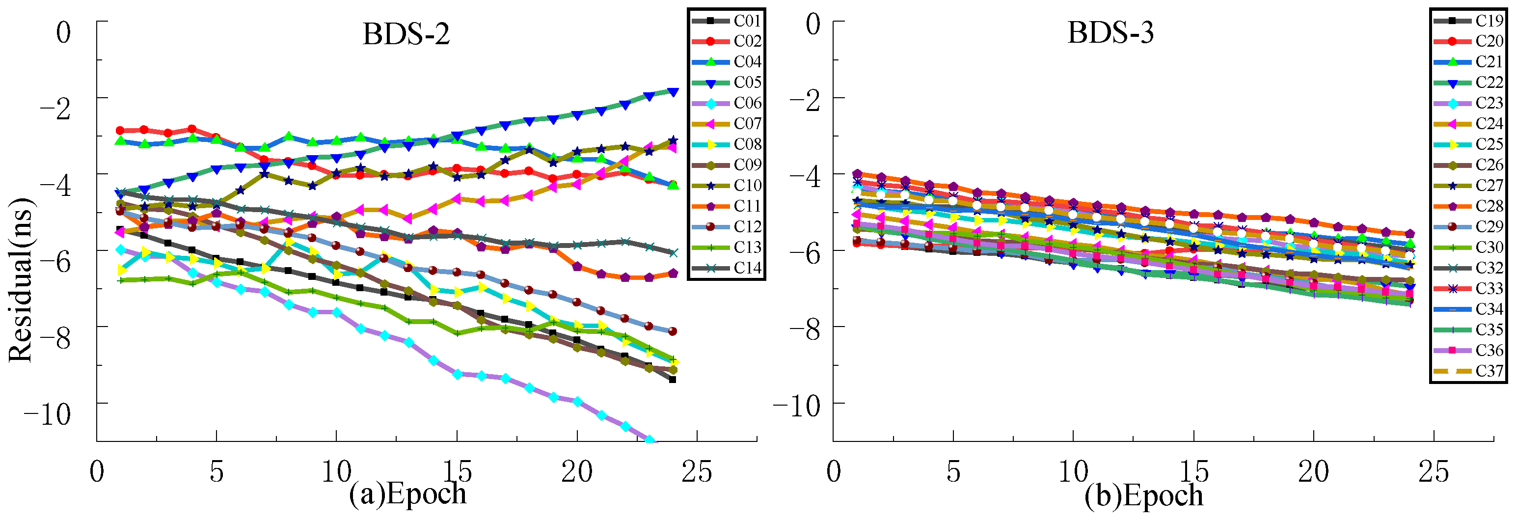
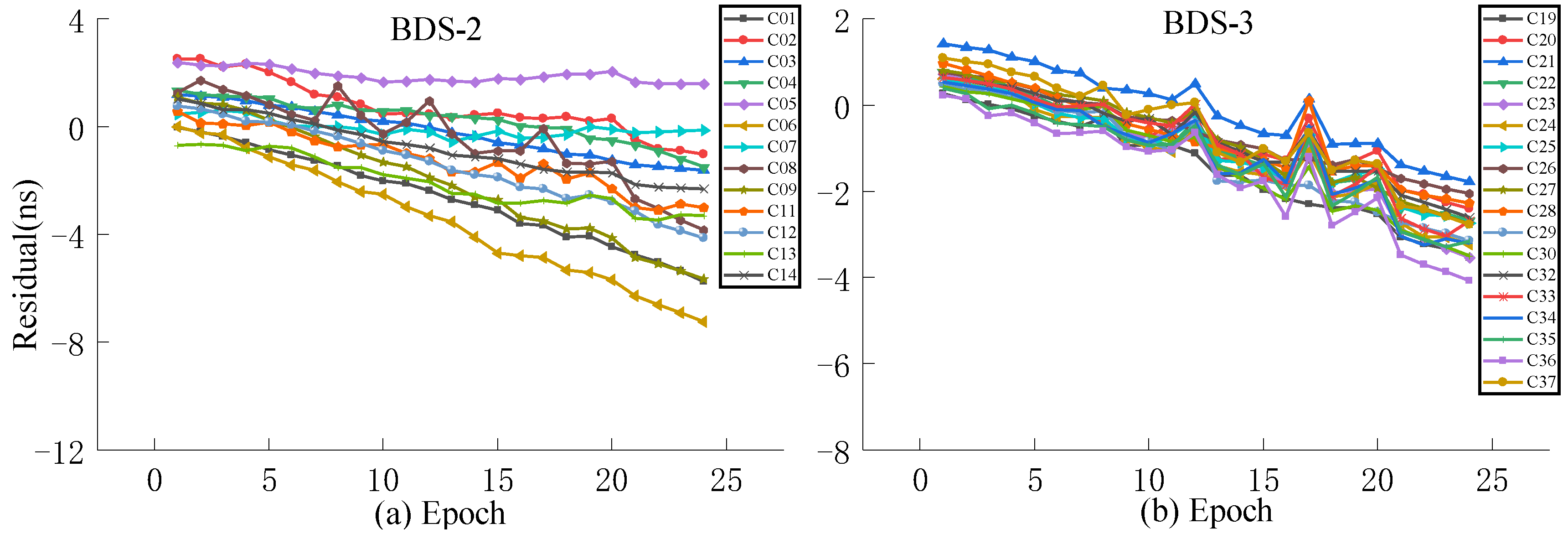
Figure 10.
The residual plot of QP model using the initial hour update ultra-fast clock product of the next day. (a) The residual value of BDS-2 predicted after 6 h. (b) The residual value of BDS-3 predicted after 6 h.
Figure 10.
The residual plot of QP model using the initial hour update ultra-fast clock product of the next day. (a) The residual value of BDS-2 predicted after 6 h. (b) The residual value of BDS-3 predicted after 6 h.
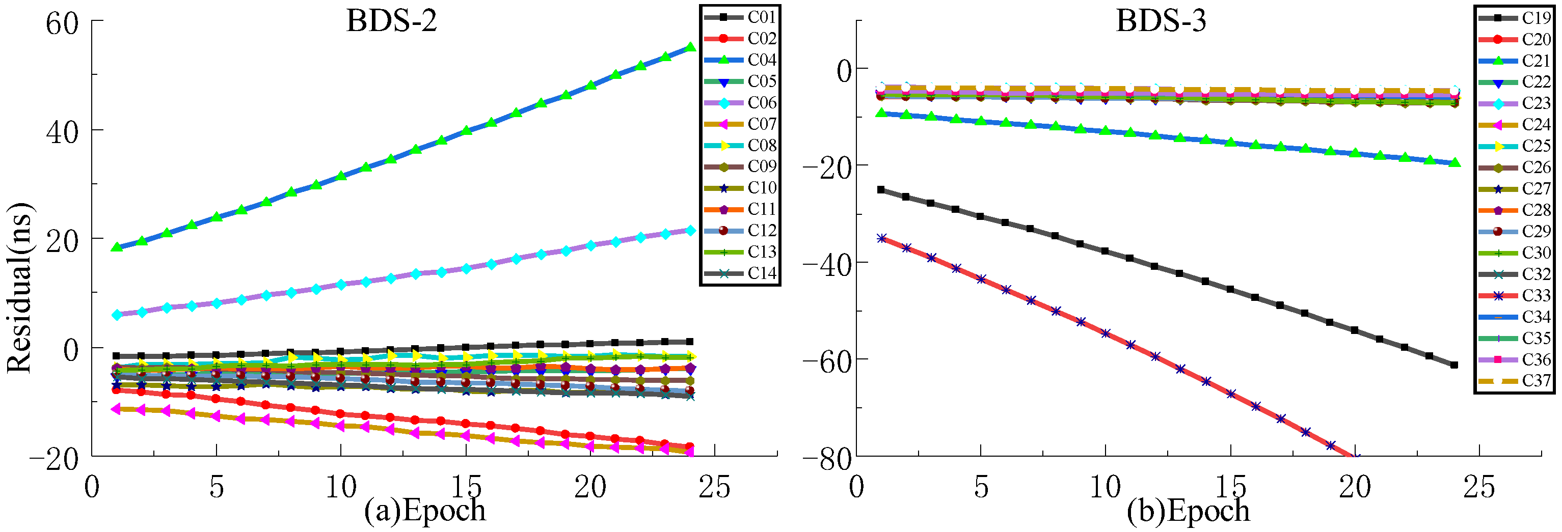
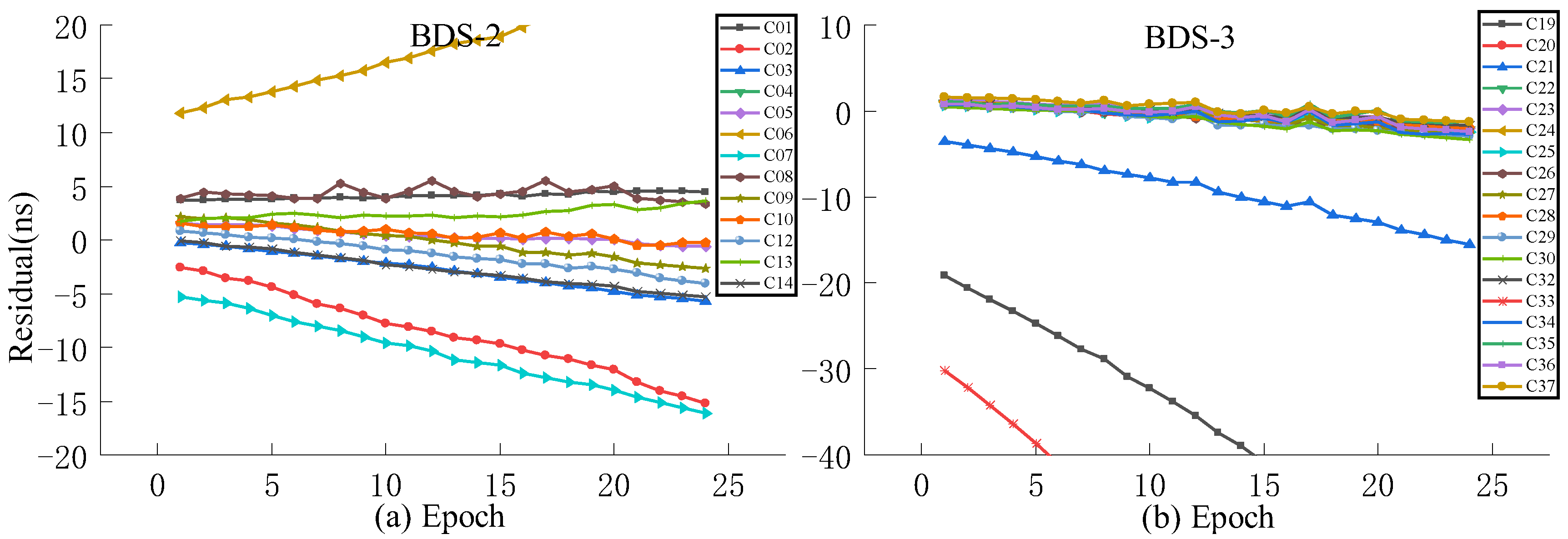
Figure 11.
The residual plot of GM model using the initial hour update ultra-fast clock product of the next day. (a) The residual value of BDS-2 predicted after 6 h. (b) The residual value of BDS-3 predicted after 6 h.
Figure 11.
The residual plot of GM model using the initial hour update ultra-fast clock product of the next day. (a) The residual value of BDS-2 predicted after 6 h. (b) The residual value of BDS-3 predicted after 6 h.
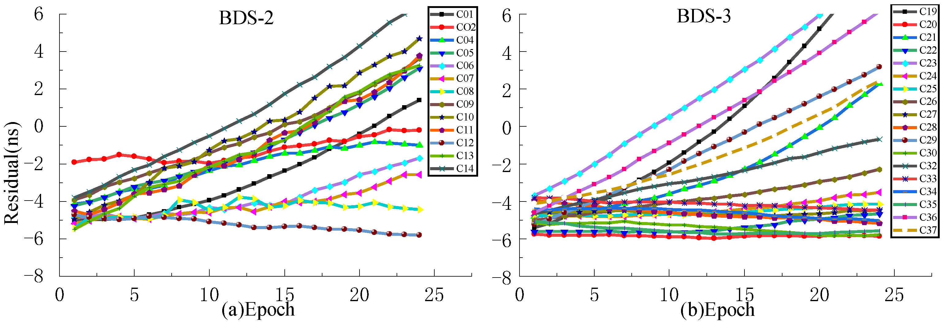
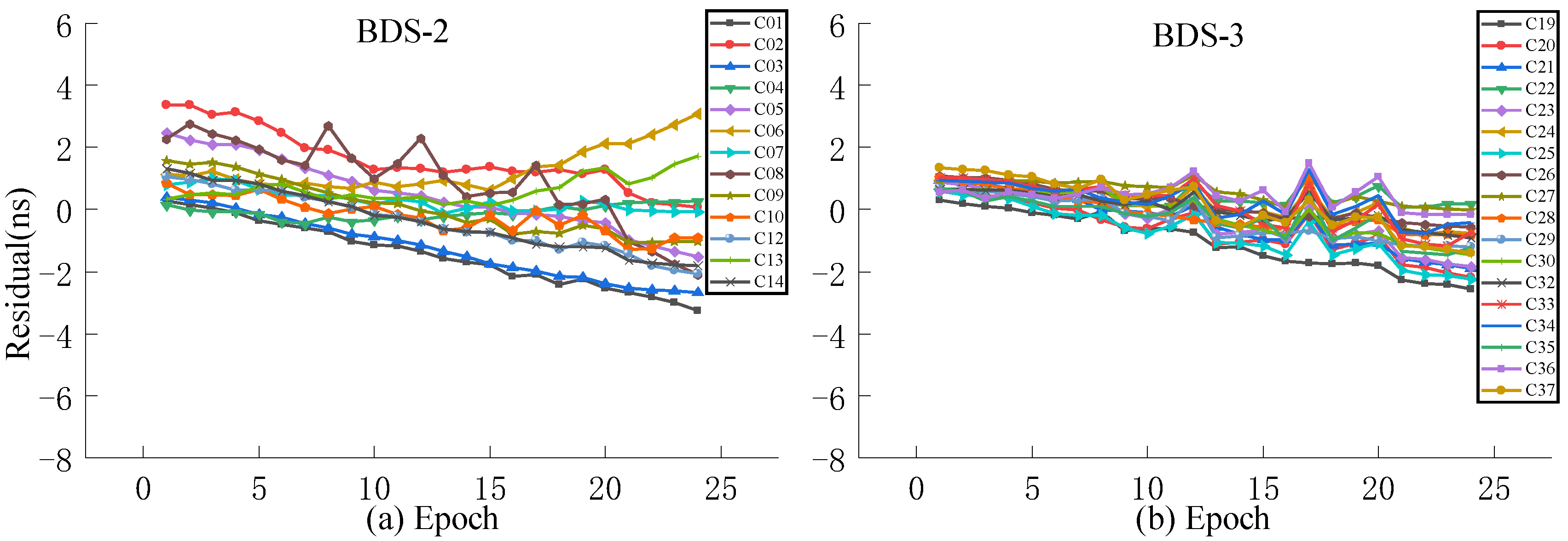
Figure 12.
The residual plot of the SSA-ELM model using the initial hour update ultra-fast clock product of the next day. (a) The residual value of BDS-2 predicted after 6 h. (b) The residual value of BDS-3 predicted after 6 h.
Figure 12.
The residual plot of the SSA-ELM model using the initial hour update ultra-fast clock product of the next day. (a) The residual value of BDS-2 predicted after 6 h. (b) The residual value of BDS-3 predicted after 6 h.
Figure 13.
The residual plot of the ISUP model using the 6th hour update ultra-fast clock product of the day. (a) The residual value of BDS-2 predicted after 6 h. (b) The residual value of BDS-3 predicted after 6 h.
Figure 13.
The residual plot of the ISUP model using the 6th hour update ultra-fast clock product of the day. (a) The residual value of BDS-2 predicted after 6 h. (b) The residual value of BDS-3 predicted after 6 h.
Figure 14.
The residual plot of the QP model using the 6th hour update ultra-fast clock product of the day. (a) The residual value of BDS-2 predicted after 6 h. (b) The residual value of BDS-3 predicted after 6 h.
Figure 14.
The residual plot of the QP model using the 6th hour update ultra-fast clock product of the day. (a) The residual value of BDS-2 predicted after 6 h. (b) The residual value of BDS-3 predicted after 6 h.
Figure 15.
The residual plot of the GM model using the 6th hour update ultra-fast clock product of the day. (a) The residual value of BDS-2 predicted after 6 h. (b) The residual value of BDS-3 predicted after 6 h.
Figure 15.
The residual plot of the GM model using the 6th hour update ultra-fast clock product of the day. (a) The residual value of BDS-2 predicted after 6 h. (b) The residual value of BDS-3 predicted after 6 h.
Figure 16.
The residual plot of the SSA-ELM model using the 6th hour update ultra-fast clock product of the day. (a) The residual value of BDS-2 predicted after 6 h. (b) The residual value of BDS-3 predicted after 6 h.
Figure 16.
The residual plot of the SSA-ELM model using the 6th hour update ultra-fast clock product of the day. (a) The residual value of BDS-2 predicted after 6 h. (b) The residual value of BDS-3 predicted after 6 h.
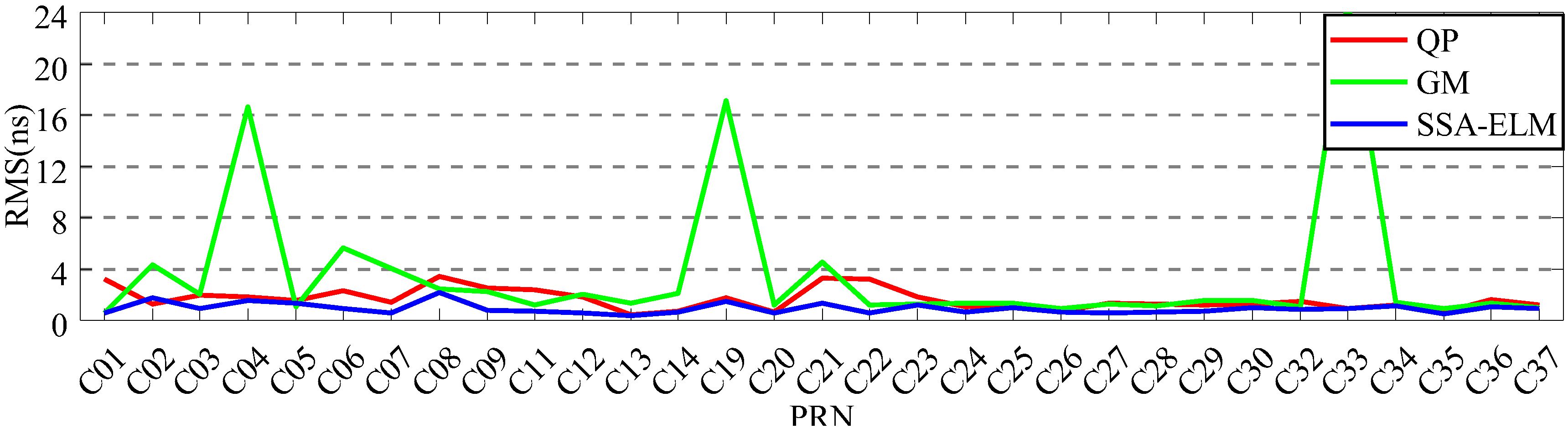
Figure 17.
The prediction accuracies of BDS for 6 h obtained using 6 h of SCB data.
Figure 17.
The prediction accuracies of BDS for 6 h obtained using 6 h of SCB data.
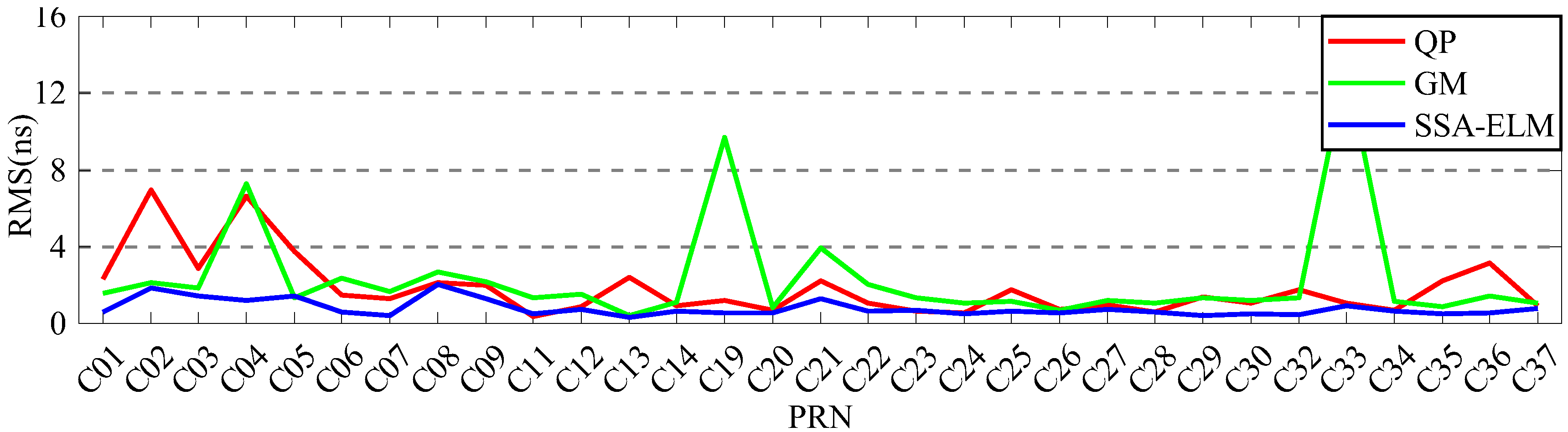
Figure 18.
The prediction accuracies of BDS for 6 h obtained using 12 h of SCB data.
Figure 18.
The prediction accuracies of BDS for 6 h obtained using 12 h of SCB data.
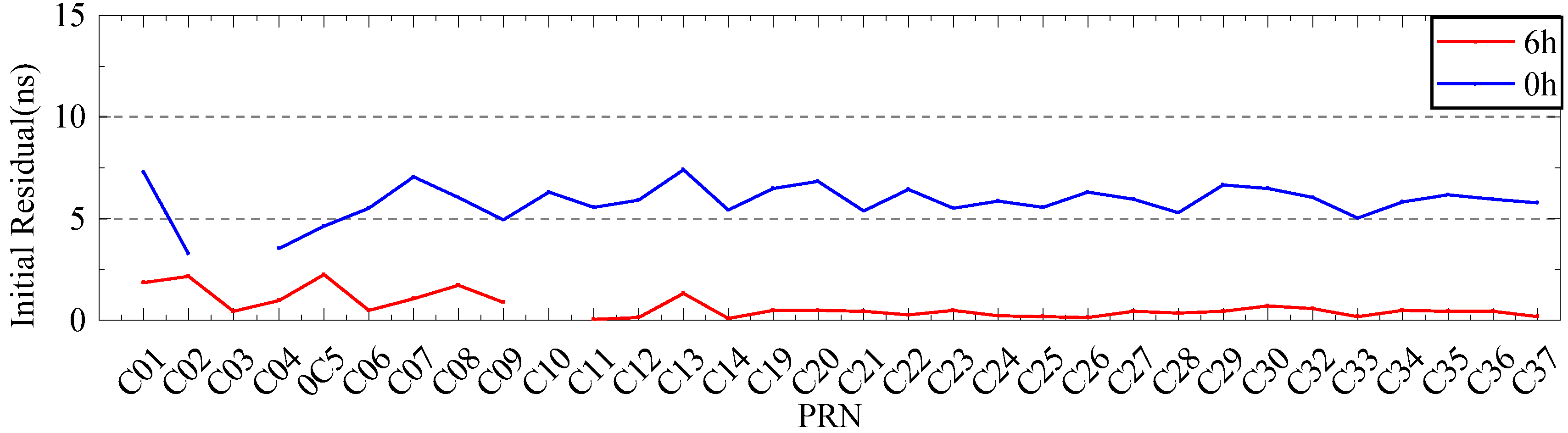
Figure 19.
The initial residual value with a DOY of 196.
Figure 19.
The initial residual value with a DOY of 196.
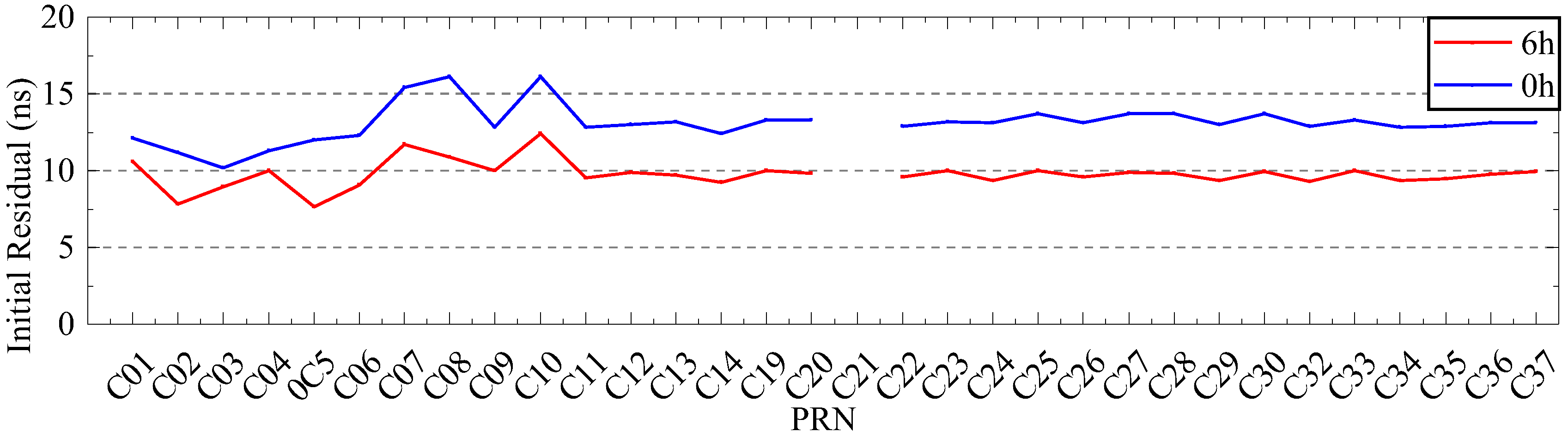
Figure 20.
The initial residual value with a DOY of 198.
Figure 20.
The initial residual value with a DOY of 198.
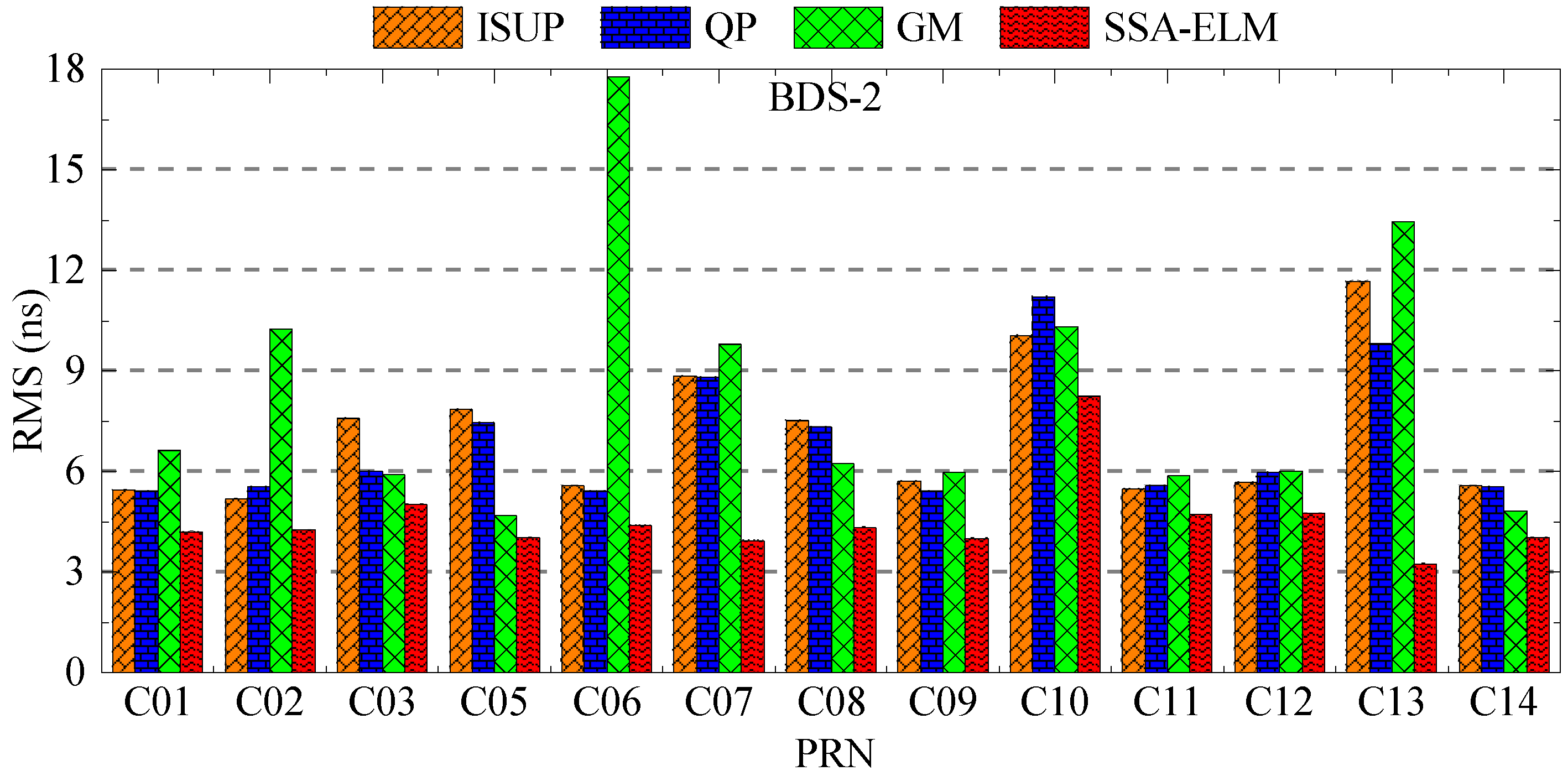
Figure 21.
Multiday average prediction accuracy of BDS-2.
Figure 21.
Multiday average prediction accuracy of BDS-2.
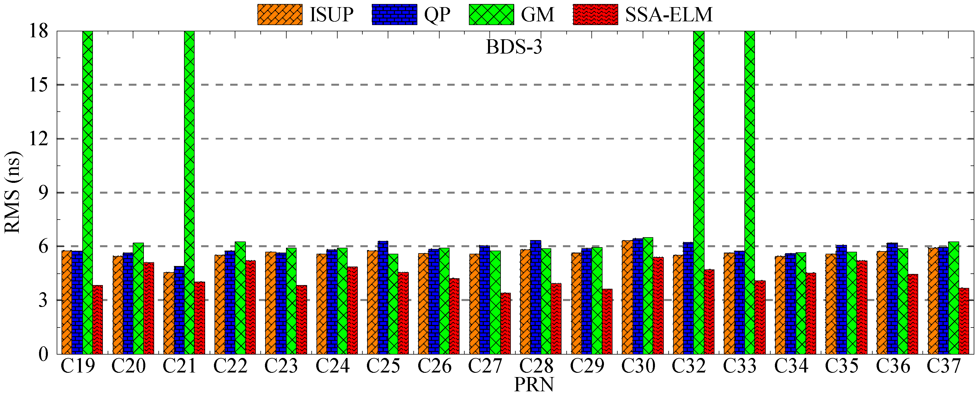
Figure 22.
Multiday average prediction accuracy of BDS-3.
Figure 22.
Multiday average prediction accuracy of BDS-3.
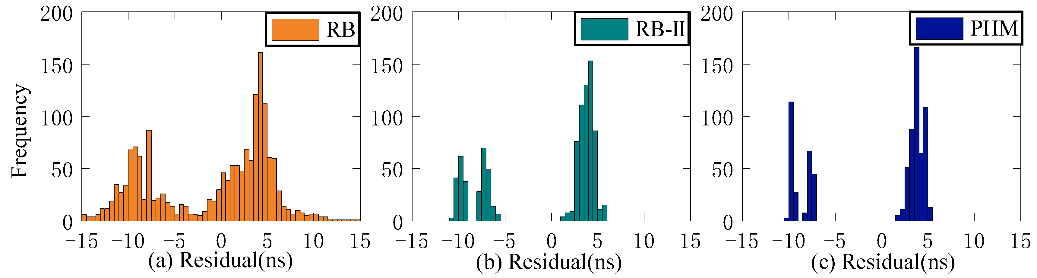
Figure 23.
Multiday prediction residual statistics of the ISUP model. (a) The residual distribution of the RB clock. (b) The residual distribution of the Rb-II clock. (c) The residual distribution of the PHM clock.
Figure 23.
Multiday prediction residual statistics of the ISUP model. (a) The residual distribution of the RB clock. (b) The residual distribution of the Rb-II clock. (c) The residual distribution of the PHM clock.
Figure 24.
Multiday prediction residual statistics of the QP model. (a) The residual distribution of the RB clock. (b) The residual distribution of the Rb-II clock. (c) The residual distribution of the PHM clock.
Figure 24.
Multiday prediction residual statistics of the QP model. (a) The residual distribution of the RB clock. (b) The residual distribution of the Rb-II clock. (c) The residual distribution of the PHM clock.
Figure 25.
Multiday prediction residual statistics of the GM model. (a) The residual distribution of the RB clock. (b) The residual distribution of the Rb-II clock. (c) The residual distribution of the PHM clock.
Figure 25.
Multiday prediction residual statistics of the GM model. (a) The residual distribution of the RB clock. (b) The residual distribution of the Rb-II clock. (c) The residual distribution of the PHM clock.
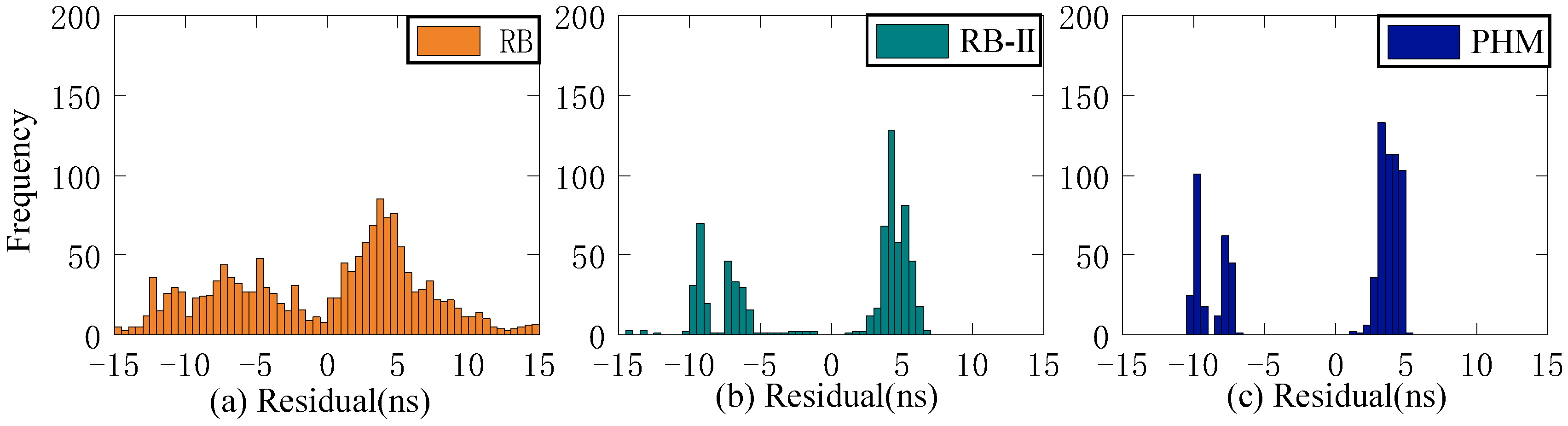
Figure 26.
Multiday prediction residual statistics of the SSA-ELM model. (a) The residual distribution of the RB clock. (b) The residual distribution of the Rb-II clock. (c) The residual distribution of the PHM clock.
Figure 26.
Multiday prediction residual statistics of the SSA-ELM model. (a) The residual distribution of the RB clock. (b) The residual distribution of the Rb-II clock. (c) The residual distribution of the PHM clock.
Table 1.
Types of BDS satellite atomic clocks used in this work.
Table 1.
Types of BDS satellite atomic clocks used in this work.
| Satellite | Clock Type | PRN |
|---|
| BDS-2 | Rb | C01, C02, C03, C04, C05, C06, C07, C08, C09, C10, C11, C12, C13, C14 |
| BDS-3 | Rb-II | C19, C20, C21, C22, C23, C24, C32, C33, C36, C37 |
| PHM | C25, C26, C27, C28, C29, C30, C34, C35 |
Table 2.
The accuracy statistics of different reference clocks (ns).
Table 2.
The accuracy statistics of different reference clocks (ns).
| Reference Clock | C11 | C20 | C27 |
|---|
| Second Difference | Rb | Rb-II | PHM | Rb | Rb-II | PHM | Rb | Rb-II | PHM |
|---|
| ISUP-ISC | 2.68 | 6.00 | 4.75 | 6.41 | 0.92 | 1.97 | 4.30 | 1.89 | 0.87 |
| ISUO-ISC | 2.60 | 5.32 | 4.18 | 5.54 | 0.89 | 1.86 | 3.61 | 1.65 | 0.68 |
| ISUP-ISUO | 1.89 | 0.83 | 0.77 | 1.78 | 0.39 | 0.42 | 1.74 | 0.46 | 0.49 |
| Mean | 2.39 | 4.05 | 3.23 | 4.58 | 0.73 | 1.42 | 3.22 | 1.33 | 0.68 |
Table 3.
The average accuracy statistics of different reference clocks for 13 days (ns).
Table 3.
The average accuracy statistics of different reference clocks for 13 days (ns).
| Reference Clock | Rb | Rb-II | PHM |
|---|
| Second Difference | Rb | Rb-II | PHM | Rb | Rb-II | PHM | Rb | Rb-II | PHM |
|---|
| ISUP-ISC | 6.74 | 5.72 | 4.49 | 9.60 | 1.10 | 2.12 | 7.58 | 2.37 | 1.41 |
| ISUO-ISC | 5.32 | 5.33 | 4.27 | 8.08 | 0.70 | 1.59 | 6.36 | 1.72 | 0.80 |
| ISUP-ISUO | 3.57 | 3.02 | 2.71 | 3.60 | 0.93 | 1.15 | 3.04 | 1.15 | 1.05 |
| Mean | 5.21 | 4.69 | 3.82 | 7.10 | 0.91 | 1.62 | 5.66 | 1.75 | 1.09 |
Table 4.
The average STD statistics of different atomic clocks (ns).
Table 4.
The average STD statistics of different atomic clocks (ns).
| Second Difference | Rb | Rb-II | PHM | Mean |
|---|
| ISUP-ISC | 3.71 | 1.41 | 0.99 | 2.03 |
| ISUO-ISC | 2.78 | 0.73 | 0.63 | 1.38 |
| ISUP-ISUO | 2.97 | 1.04 | 0.91 | 1.64 |
| Mean | 3.15 | 1.06 | 0.84 | |
Table 5.
The average RMS values of 3 h for different prediction models based on 24 h of SCB data (ns).
Table 5.
The average RMS values of 3 h for different prediction models based on 24 h of SCB data (ns).
| Model | ISUP | QP | GM | SSA-ELM | Enhancement with ISUP (%) | Enhancement with QP (%) | Enhancement with GM (%) |
|---|
| Rb | 1.75 | 1.09 | 2.88 | 0.97 | 44.67 | 11.58 | 66.32 |
| Rb-II | 1.65 | 0.56 | 1.37 | 0.55 | 66.57 | 1.99 | 59.85 |
| PHM | 1.62 | 0.50 | 0.50 | 0.49 | 70.01 | 2.81 | 3.20 |
| Mean | 1.67 | 0.72 | 1.58 | 0.67 | 60.42 | 5.46 | 57.59 |
Table 6.
The average RMS values of 6 h for different prediction models based on 24 h of SCB data (ns).
Table 6.
The average RMS values of 6 h for different prediction models based on 24 h of SCB data (ns).
| Model | ISUP | QP | GM | SSA-ELM | Enhancement with ISUP (%) | Enhancement with QP (%) | Enhancement with GM (%) |
|---|
| Rb | 3.19 | 1.88 | 3.93 | 1.13 | 64.66 | 39.93 | 71.25 |
| Rb-II | 3.35 | 1.48 | 2.09 | 0.80 | 76.04 | 45.71 | 61.72 |
| PHM | 3.19 | 1.48 | 1.27 | 0.76 | 76.10 | 48.31 | 40.05 |
| Mean | 3.25 | 1.61 | 2.43 | 0.90 | 72.27 | 44.65 | 62.96 |
Table 7.
The average RMS values of 6 h for three prediction models based on 6 h of SCB data (ns).
Table 7.
The average RMS values of 6 h for three prediction models based on 6 h of SCB data (ns).
| Model | QP | GM | SSA-ELM | Enhancement with QP (%) | Enhancement with GM (%) |
|---|
| Rb | 2.62 | 2.12 | 1.01 | 61.43 | 52.35 |
| Rb-II | 1.34 | 1.64 | 0.71 | 47.21 | 56.79 |
| PHM | 1.17 | 1.09 | 0.58 | 50.84 | 47.14 |
| Mean | 1.71 | 1.62 | 0.76 | 53.16 | 52.09 |
Table 8.
The average RMS values of 6 h for three prediction models based on 12 h of SCB data (ns).
Table 8.
The average RMS values of 6 h for three prediction models based on 12 h of SCB data (ns).
| Model | QP | GM | SSA-ELM | Enhancement with QP (%) | Enhancement with GM (%) |
|---|
| Rb | 1.89 | 2.40 | 0.97 | 48.33 | 59.40 |
| Rb-II | 1.68 | 1.60 | 0.93 | 44.56 | 41.46 |
| PHM | 1.08 | 1.24 | 0.77 | 29.08 | 38.28 |
| Mean | 1.55 | 1.75 | 0.89 | 40.66 | 46.38 |
Table 9.
The statistics of the average RMS values of initial residuals in different clock bias files.
Table 9.
The statistics of the average RMS values of initial residuals in different clock bias files.
| Clock Type | Rb | Rb-II | PHM | Mean |
|---|
| 0h | 9.75 | 9.42 | 9.64 | 9.60 |
| 6h | 5.16 | 4.96 | 5.13 | 5.08 |
Table 10.
The average RMS values of 6 days for three different prediction models (ns).
Table 10.
The average RMS values of 6 days for three different prediction models (ns).
| Model | ISUP | QP | GM | SSA-ELM | Enhancement with ISUP (%) | Enhancement with QP (%) | Enhancement with GM (%) |
|---|
| Rb | 7.08 | 6.88 | 7.50 | 4.54 | 35.90 | 33.98 | 39.43 |
| Rb-II | 5.54 | 5.76 | 6.07 | 4.39 | 20.79 | 23.86 | 27.72 |
| PHM | 5.72 | 6.06 | 5.86 | 4.36 | 23.86 | 28.17 | 25.72 |
| Mean | 6.11 | 6.23 | 6.48 | 4.43 | 26.85 | 28.67 | 30.96 |

 ,
, 


