
Real-Time Compensation for SLD Light-Power Fluctuation in an Interferometric Fiber-Optic Gyroscope

Abstract
:1. Introduction
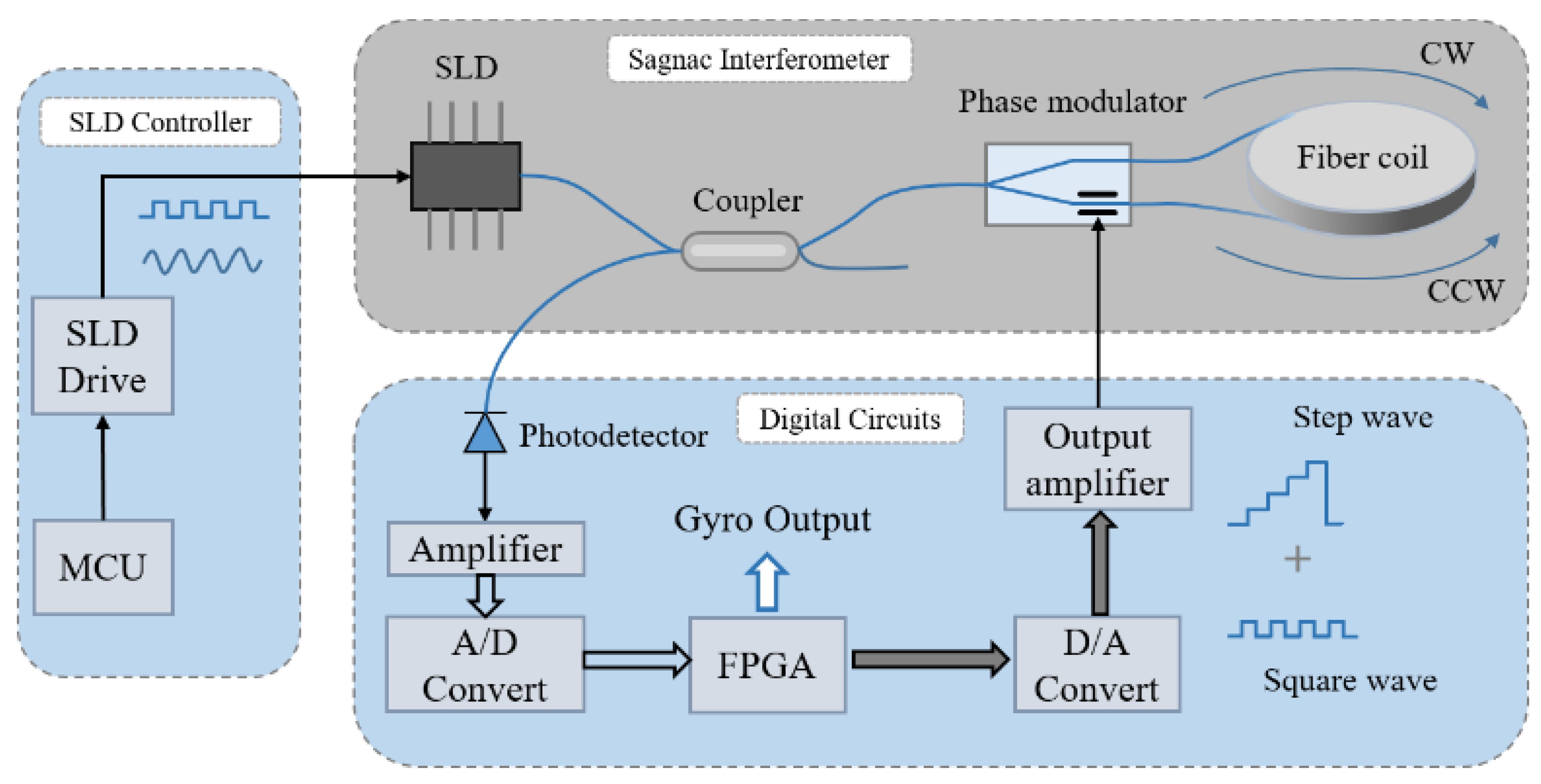
2. Basic Principles of Closed-Loop IFOGs
3. Analysis
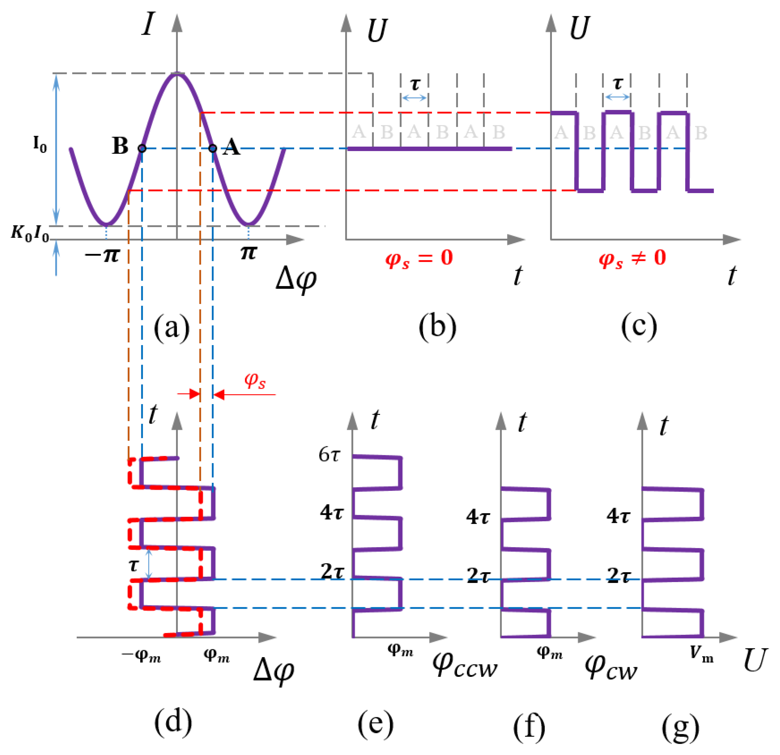
3.1. Principle of Error Generation
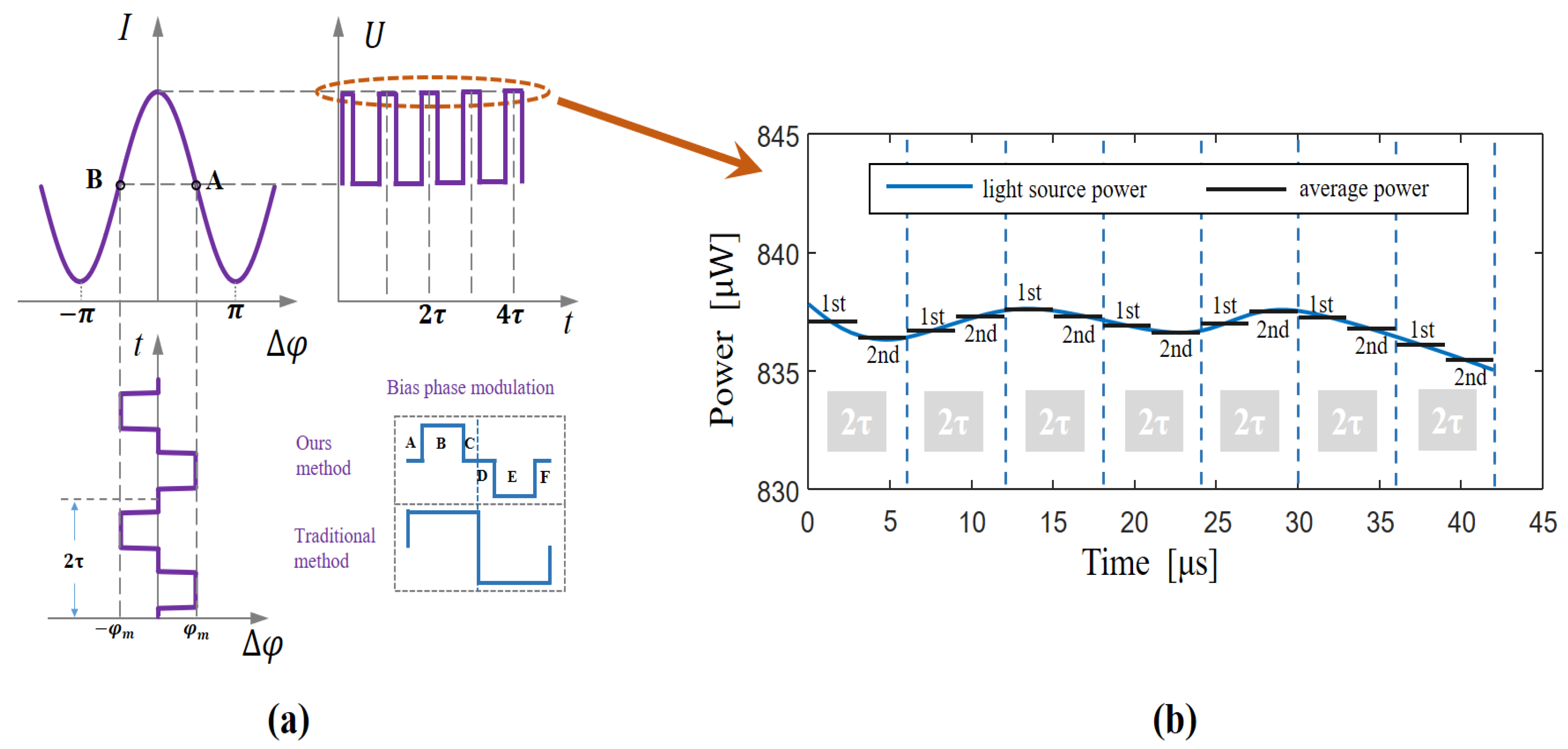
3.2. Light-Source Power Signal Demodulation Method
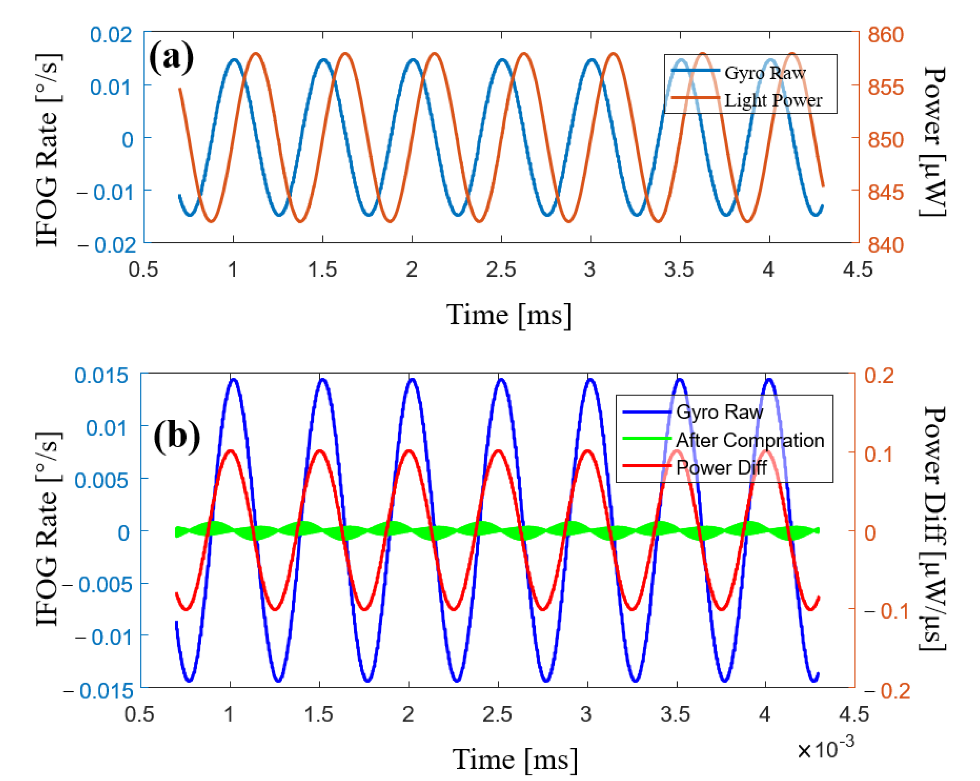
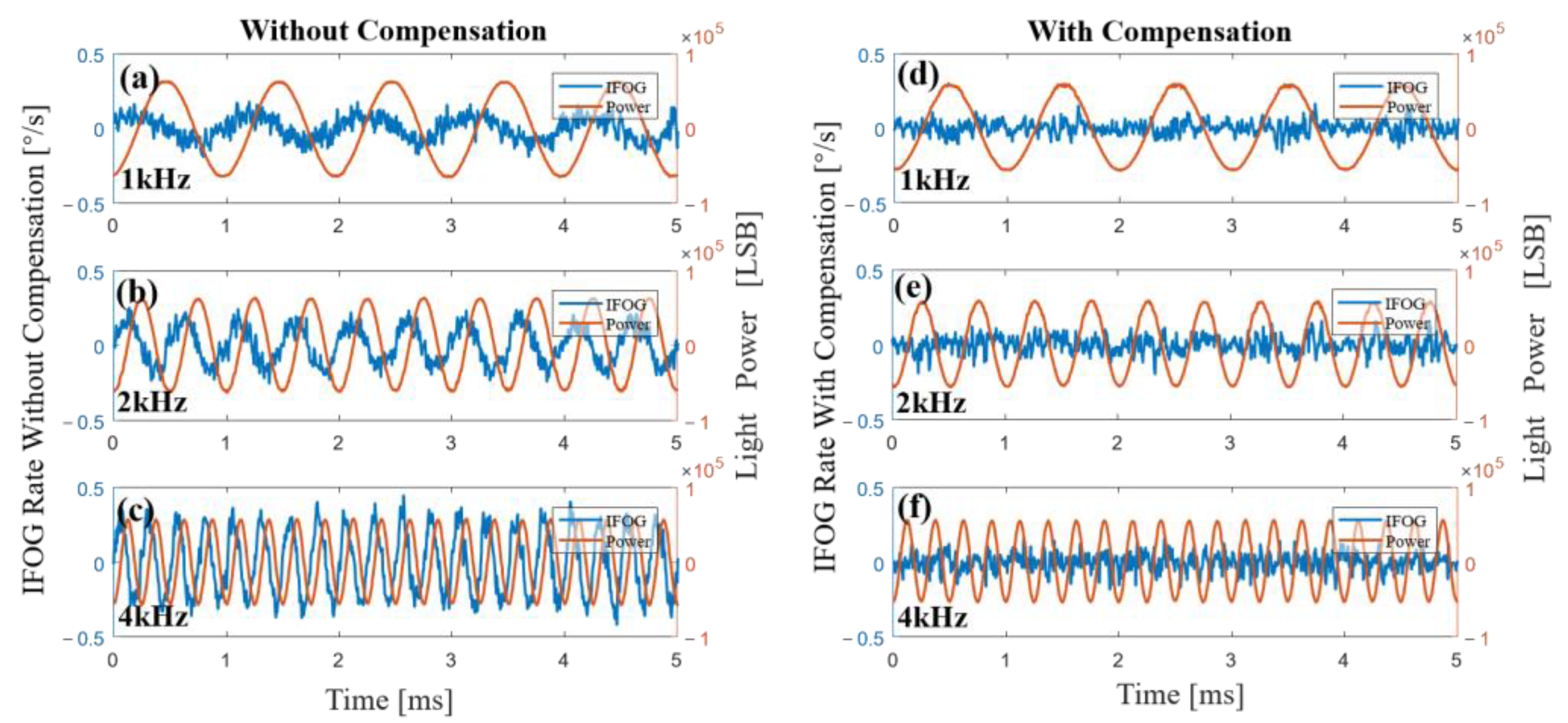
3.3. Error Compensation Simulations
4. Experimental Section
4.1. Demodulation of the Light-Source Power Signal
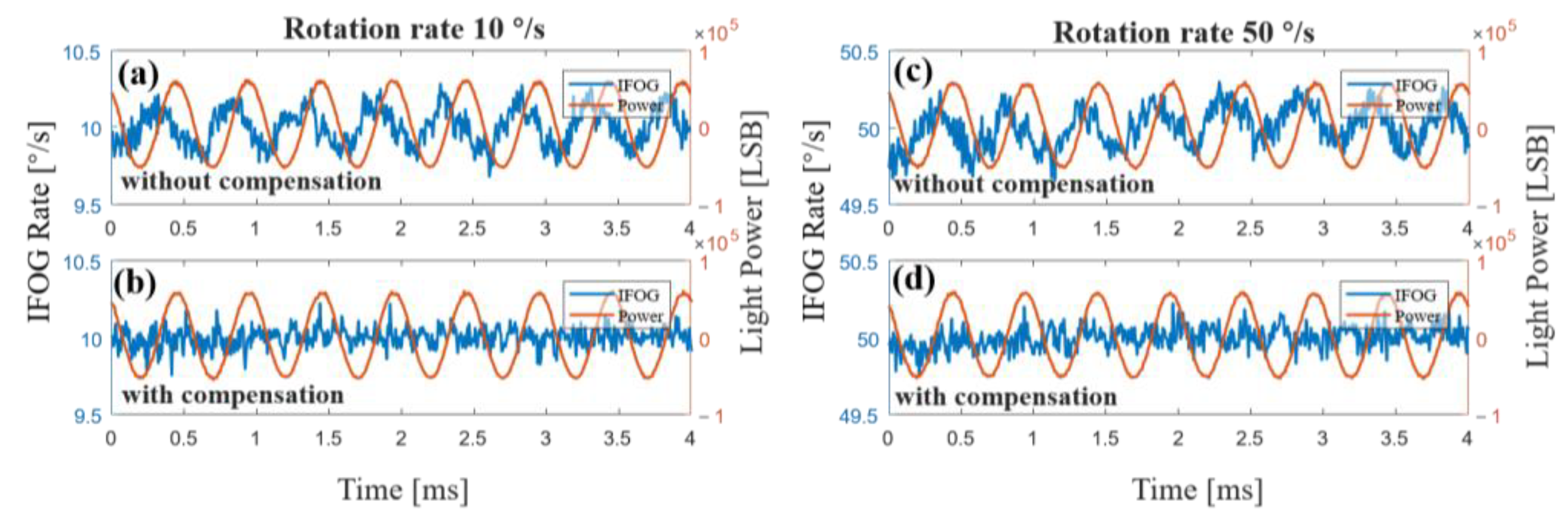
4.2. Error Compensation
5. Conclusions
Author Contributions
Funding
Institutional Review Board Statement
Informed Consent Statement
Data Availability Statement
Conflicts of Interest
References
- Mao, N.; Xu, J.; Li, J.; He, H. A LSTM-RNN-based fiber optic gyroscope drift compensation. Math. Probl. Eng. 2021, 2021, 1636001. [Google Scholar] [CrossRef]
- Wang, Z.; Wang, G.; Kumar, S.; Marques, C.; Min, R.; Li, X. Recent advancements in resonant fiber optic gyro—A Review. IEEE Sens. J. 2022, 22, 18240–18252. [Google Scholar] [CrossRef]
- Shang, K.; Lei, M.; Xiang, Q.; Na, Y.; Zhang, L. Tactical-grade interferometric fiber optic gyroscope based on an integrated optical chip. Opt. Commun. 2021, 485, 126729. [Google Scholar] [CrossRef]
- Zhao, S.; Zhou, Y.; Shu, X. Study on nonlinear error calibration of fiber optical gyroscope scale factor based on LSTM. Measurement 2022, 190, 110783. [Google Scholar] [CrossRef]
- Li, X.; Liu, P.; Guang, X.; Xu, Z.; Guan, L.; Li, G. Temperature dependence of faraday effect-induced bias error in a fiber optic gyroscope. Sensors 2017, 17, 2046. [Google Scholar] [CrossRef]
- Chen, X.; Jiang, L.; Yang, M.; Yang, J.; Shu, X. Research on the mean-wavelength drift mechanism of SLD light source in FOG. J. Phys. Conf. Ser. 2019, 1300, 012047. [Google Scholar] [CrossRef]
- Zhang, C.; Zhang, S.; Pan, X.; Jin, J. Six-state phase modulation for reduced crosstalk in a fiber optic gyroscope. Opt. Express 2018, 26, 10535–10549. [Google Scholar] [CrossRef]
- Skalský, M.; Havránek, Z.; Fialka, J. Efficient Modulation and Processing Method for Closed-Loop Fiber Optic Gyroscope with Piezoelectric Modulator. Sensors 2019, 19, 1710. [Google Scholar] [CrossRef]
- Hui, F.; Tianjin, M.L.; Ma, L.; Zuo, W.; Zhang, S.; Zhang, X.M. Investigation on near Gaussian-shaped spectrum erbium-doped fiber source which applied to the fiber optic gyroscope. In Proceedings of the 2017 24th Saint Petersburg International Conference on Integrated Navigation Systems (ICINS), Saint Petersburg, Russia, 29–31 May 2017; pp. 1–4. [Google Scholar]
- Fei, H.; Mao-chun, L.; Lin, M. Double-Pass Backward ASE light source which applied to the three-axis FOG. J. Chin. Inert. Technol. 2016, 24, 158–162. [Google Scholar]
- Chen, X.; Yang, J.; Zhou, Y.; Shu, X. An improved temperature compensation circuit for SLD light source of fiber-optic gyroscope. J. Phys. Conf. Ser. 2017, 916, 012027. [Google Scholar] [CrossRef]
- Ji, Z.; Ma, C. The novel stable control scheme of the light source power in the closed-loop fiber optic gyroscope. J. Phys. Conf. Ser. 2011, 276, 012127. [Google Scholar] [CrossRef] [Green Version]
- Zhang, F.; Wang, Y.; Lin, X.; Cheng, Y.; Zhang, Z.; Liu, Y.; Liao, L.; Xing, Y.; Yang, L.; Dai, N.; et al. Gain-tailored Yb/Ce codoped aluminosilicate fiber for laser stability improvement at high output power. Opt. Express 2019, 27, 20824–20836. [Google Scholar] [CrossRef] [PubMed]
- Yan, J.; Miao, L.; Chen, M.; Huang, T.; Che, S.; Shu, X. Research on the feedback control characteristics and parameter optimization of closed-loop fiber optic gyroscope. Optik 2021, 229, 166298. [Google Scholar] [CrossRef]
- Komljenovic, T.; Bowers, J.E. High temperature stability, low coherence and low relative intensity noise semiconductor sources for interferometric sensors. Opt. Express 2016, 24, 22777–22787. [Google Scholar] [CrossRef] [PubMed]
- Xue, L.; Zhou, Y.; Li, J.; Liu, W.; Xing, E.; Chen, J.; Tang, J.; Liu, J. Error analysis of dual-polarization fiber optic gyroscope under the magnetic field-variable temperature field. Opt. Fiber Technol. 2022, 71, 102926. [Google Scholar] [CrossRef]
- Cao, Y.; Xu, W.; Lin, B.; Zhu, Y.; Meng, F.; Zhao, X.; Ding, J.; Lian, Z.; Xu, Z.; Yu, Q. A method for temperature error compensation in fiber-optic gyroscope based on machine learning. Optik 2022, 256, 168765. [Google Scholar] [CrossRef]
- Li, J.; Zhou, Y.; Xue, L.; Liu, W.; Xing, E.; Tang, J.; Liu, J. Magnetic error suppression in Polarization-Maintaining fiber optic gyro system with orthogonal polarization states. Opt. Fiber Technol. 2022, 71, 102927. [Google Scholar] [CrossRef]
- Bischel, W.K.; Kouchnir, M.A.; Bitter, M.; Yahalom, R.; Taylor, E.W. Hybrid integration of fiber optic gyroscopes operating in harsh environments. In Nanophotonics and Macrophotonics for Space Environments V; SPIE: Saint-Denis, France, 2011; pp. 197–204. [Google Scholar]
- Zhang, C.; Song, N.; Li, L.; Jin, J.; Yang, D.; Xu, H. Fiber optic gyro R&D at Beihang University. In Proceedings of the OFS2012 22nd International Conference on Optical Fiber Sensors, Beijing, China, 14 October 2012; pp. 71–74. [Google Scholar]
- Pan, X.; Liu, P.; Zhang, S.; Jin, J.; Song, N. Novel Compensation Scheme for the Modulation Gain to Suppress the Quantization-Induced Bias in a Fiber Optic Gyroscope. Sensors 2017, 17, 823. [Google Scholar] [CrossRef]
- Liu, D.; Li, H.; Wang, X.; Liu, H.; Ni, P.; Liu, N.; Feng, L. Interferometric optical gyroscope based on an integrated silica waveguide coil with low loss. Opt. Express 2020, 28, 15718–15730. [Google Scholar] [CrossRef]
- Wang, L.; Halstead, D.R.; Monte, T.D.; Khan, J.A.; Brunner, J.; Heyningen, M.A.K.v. Low-cost, High-end Tactical-grade Fiber Optic Gyroscope Based on Photonic Integrated Circuit. In Proceedings of the 2019 IEEE International Symposium on Inertial Sensors and Systems (INERTIAL), Naples, FL, USA, 1–5 April 2019; pp. 1–2. [Google Scholar]
- Lefevre, H.C. Application of the Sagnac effect in the interferometric fiber-optic gyroscope. Opt. Gyros Appl. 1999, 45, 7. [Google Scholar]
- Vali, V.; Shorthill, R.W. Fiber ring interferometer. Appl. Opt. 1976, 15, 1099–1100. [Google Scholar] [CrossRef] [PubMed]
- Zhang, G.-C. The Principles and Technologies of Fiber-Optic Gyroscope; National Defense Industry Press: Beijing, China, 2008; pp. 244–251. [Google Scholar]
- Li, X.; Zhang, Y.; Zhang, C. Five Points Modulation in Closed Loop Fiber Optic Gyroscope. In Proceedings of the 2009 5th International Conference on Wireless Communications, Networking and Mobile Computing, Beijing, China, 24–26 September 2009; pp. 1–3. [Google Scholar]


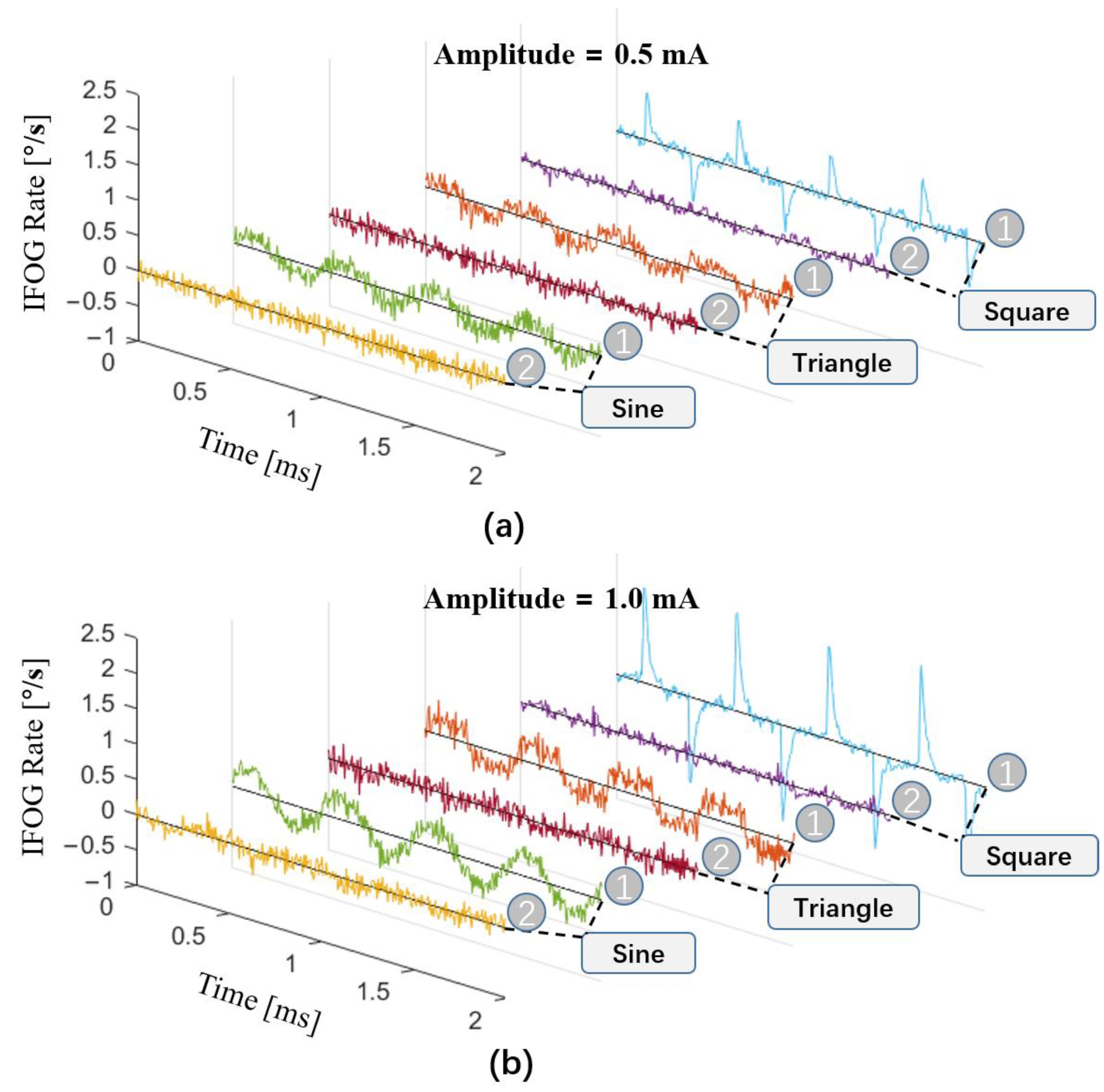
| Waveform | Frequency | Amplitude |
|---|---|---|
| Square | 2 kHz | 0.5 mA |
| Triangle | 1.0 mA | |
| Sine |
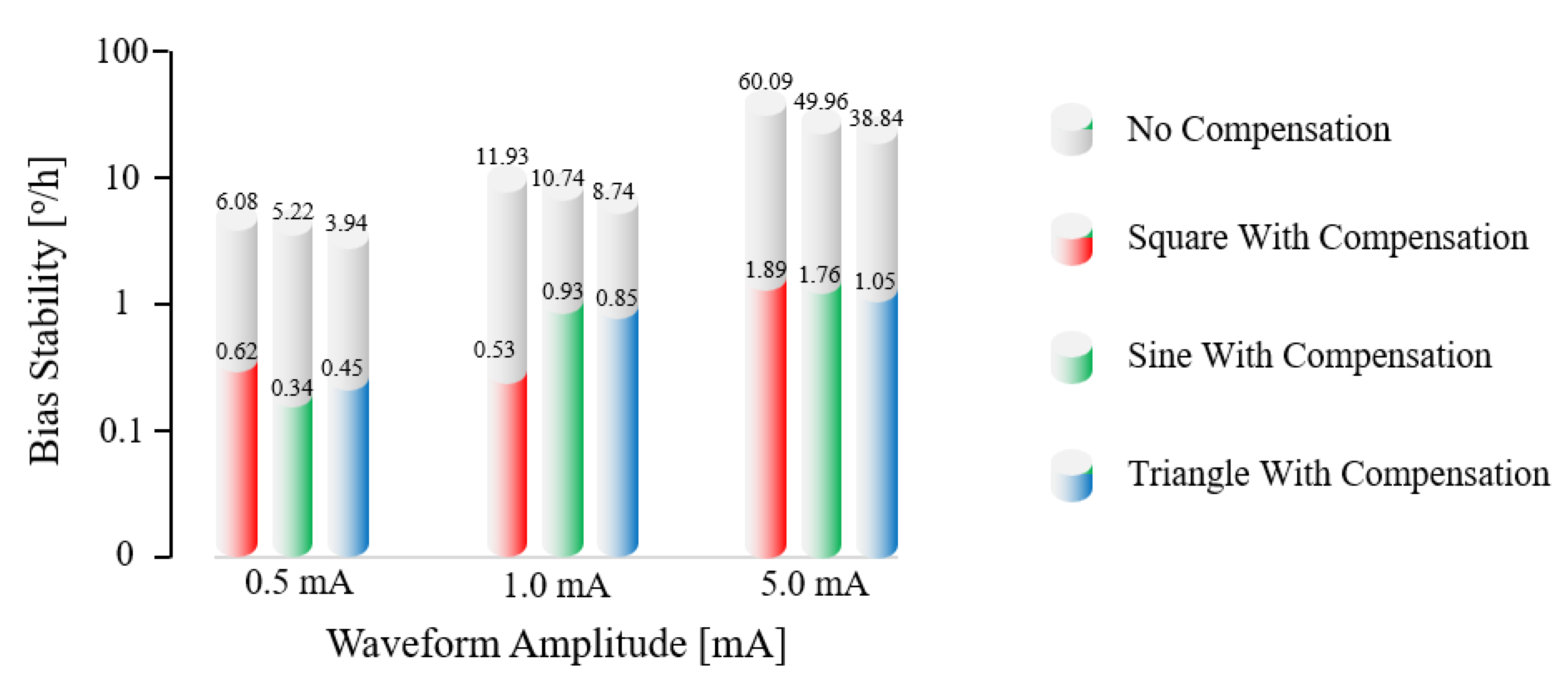
| Waveform | Amplitude (mA) | Stability without Compensation (°/h) | Stability with Compensation (°/h) | Percentage of Improvement |
|---|---|---|---|---|
| Constant | \ | 0.0885 | 0.0874 | 1.2% |
| Square | 0.5 | 6.08 | 0.62 | 89.8% |
| Sine | 0.5 | 5.22 | 0.34 | 93.5% |
| Triangle | 0.5 | 3.94 | 0.45 | 88.6% |
| Square | 1.0 | 11.93 | 0.53 | 95.6% |
| Sine | 1.0 | 10.74 | 0.93 | 91.3% |
| Triangle | 1.0 | 8.74 | 0.85 | 90.3% |
| Square | 5.0 | 60.09 | 1.89 | 96.9% |
| Sine | 5.0 | 49.96 | 1.76 | 96.5% |
| Triangle | 5.0 | 38.84 | 1.05 | 97.3% |
Disclaimer/Publisher’s Note: The statements, opinions and data contained in all publications are solely those of the individual author(s) and contributor(s) and not of MDPI and/or the editor(s). MDPI and/or the editor(s) disclaim responsibility for any injury to people or property resulting from any ideas, methods, instructions or products referred to in the content. |
© 2023 by the authors. Licensee MDPI, Basel, Switzerland. This article is an open access article distributed under the terms and conditions of the Creative Commons Attribution (CC BY) license (https://creativecommons.org/licenses/by/4.0/).
Share and Cite
Zheng, S.; Ren, M.; Luo, X.; Zhang, H.; Feng, G. Real-Time Compensation for SLD Light-Power Fluctuation in an Interferometric Fiber-Optic Gyroscope. Sensors 2023, 23, 1925. https://doi.org/10.3390/s23041925
Zheng S, Ren M, Luo X, Zhang H, Feng G. Real-Time Compensation for SLD Light-Power Fluctuation in an Interferometric Fiber-Optic Gyroscope. Sensors. 2023; 23(4):1925. https://doi.org/10.3390/s23041925
Chicago/Turabian StyleZheng, Shijie, Mengyu Ren, Xin Luo, Hangyu Zhang, and Guoying Feng. 2023. "Real-Time Compensation for SLD Light-Power Fluctuation in an Interferometric Fiber-Optic Gyroscope" Sensors 23, no. 4: 1925. https://doi.org/10.3390/s23041925