
An Unsupervised Learning Approach for Wayside Train Wheel Flat Detection


 , , , and
Abstract
:1. Introduction
- (1)
- Development of an unsupervised data-driven methodology using acceleration responses on the rail for detecting defective wheels from healthy ones;
- (2)
- Implementation of AR, ARX, CWT, and PCA for feature extraction from multiple sensors to transform the time series measurements into damage-sensitive features, where the correlation with the damage can be more easily observed;
- (3)
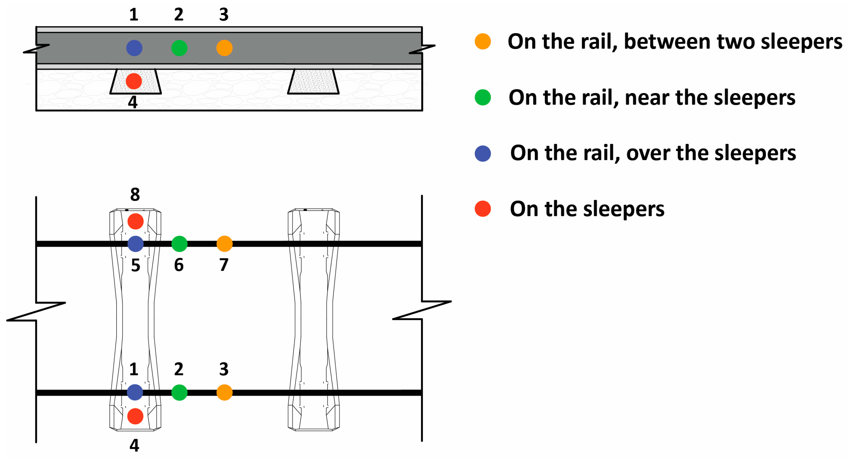
- Analysis of the performance of the four feature extraction methods considering the different number and locations of the sensors on the rails;
- (4)
- Comparison of the sensitivity of the proposed methodologies to the side (left vs. right) of the defective wheel in a train axle;
- (5)
- Evaluation of the effectiveness of the proposed method with respect to the minimalist layout of sensors;
- (6)
- Improvement in wheel flat detection by applying a two-stage fusion process: in the first step, the features from each sensor are merged and, in the second stage, the multi-sensor information is fused to enhance the sensibility to the damage.
2. Numerical Simulation
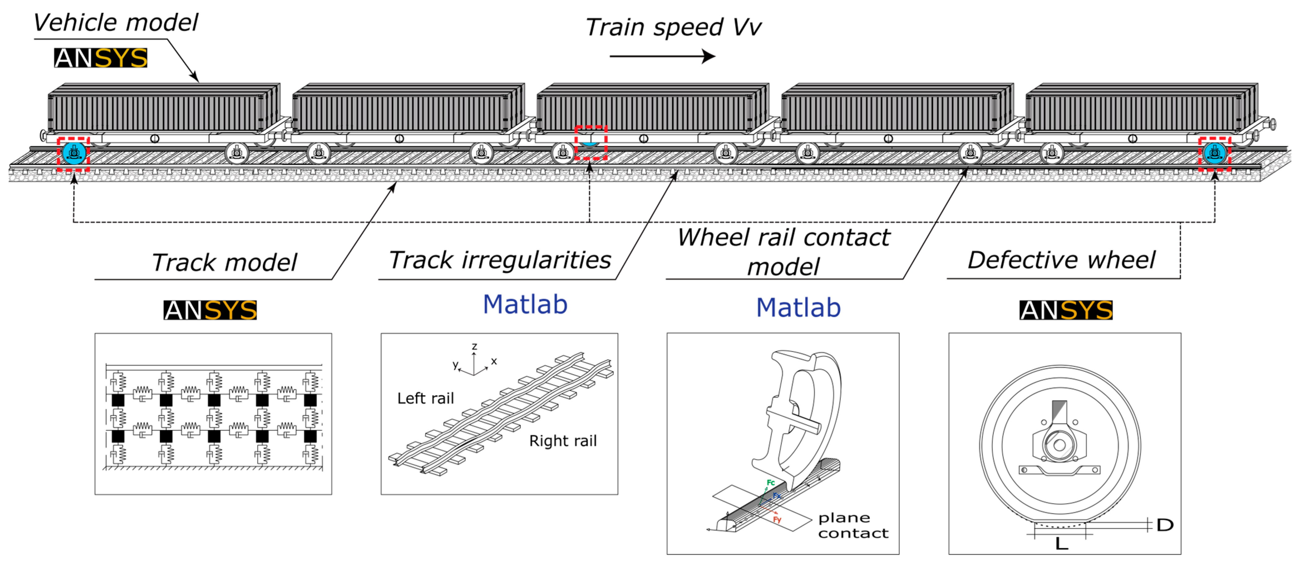
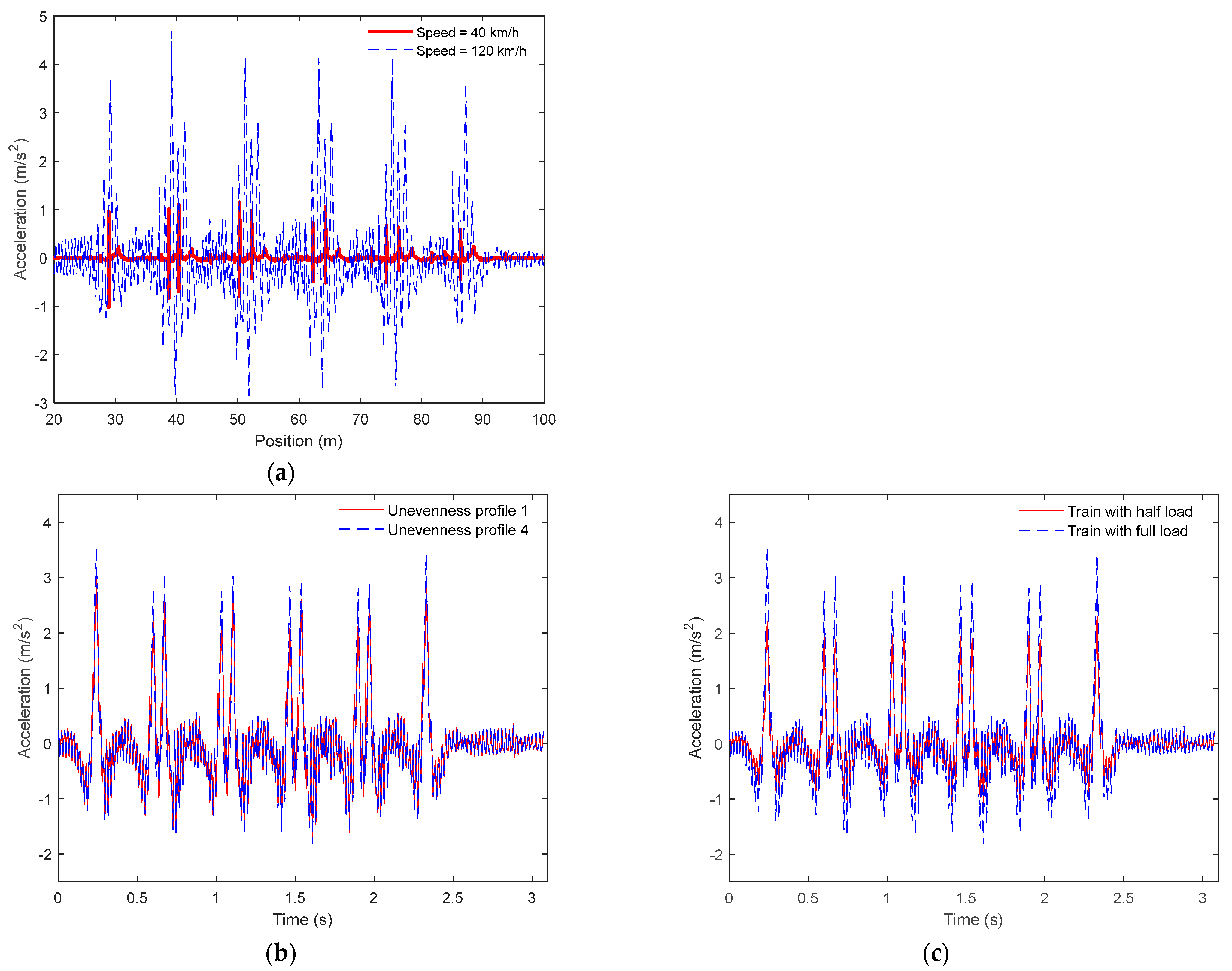
2.1. Train–Track Dynamic Interaction
2.2. Virtual Wayside System
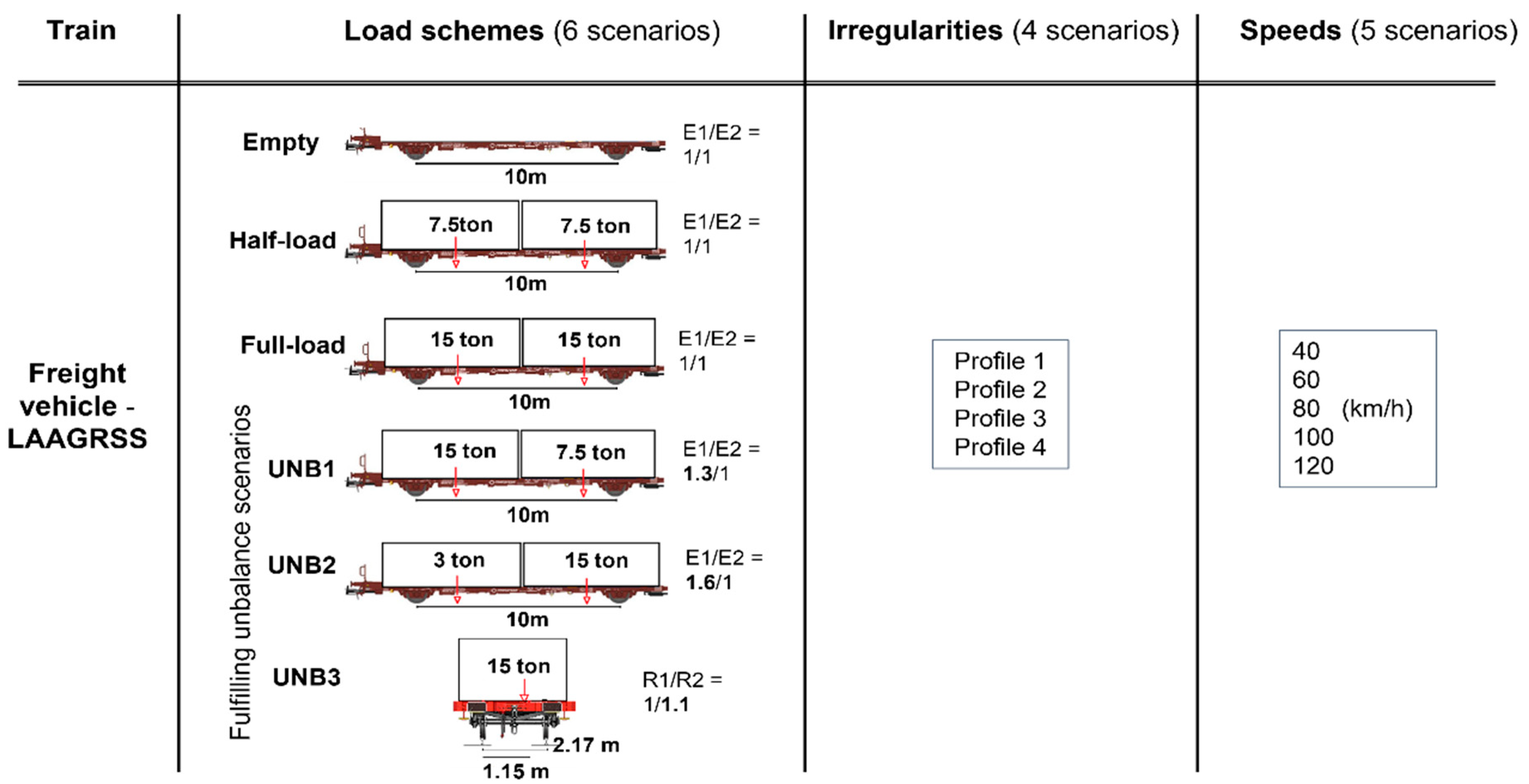
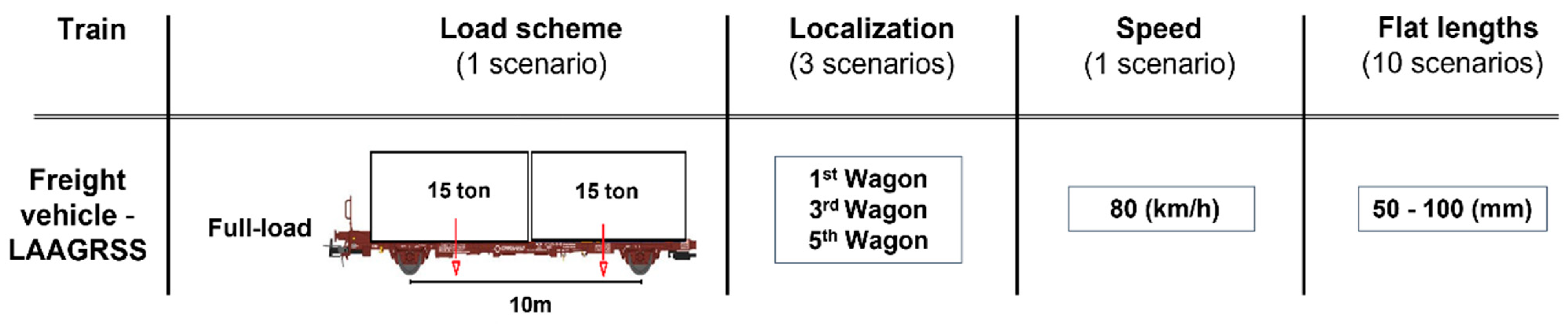
2.3. Baseline and Damaged Scenarios
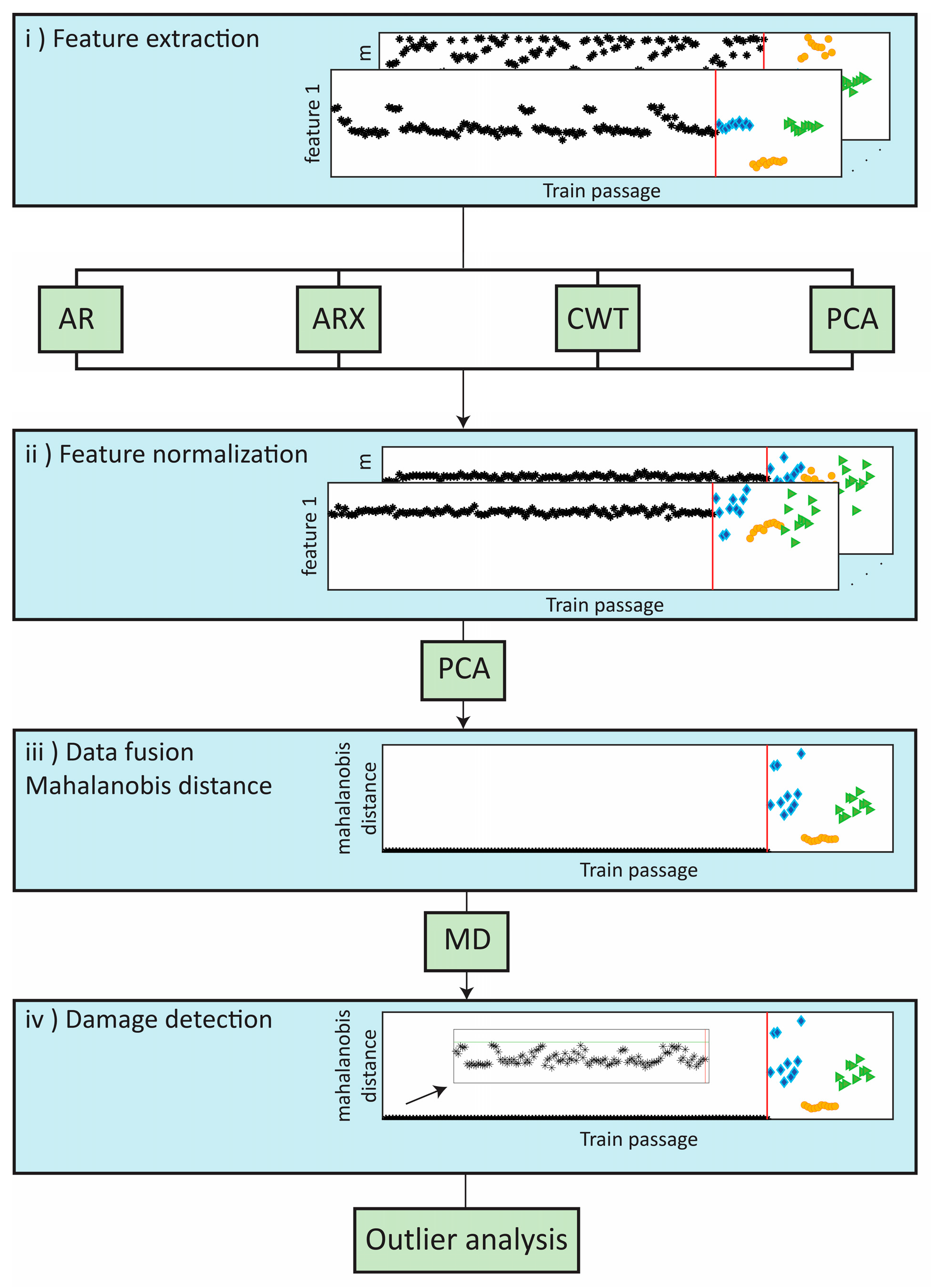
3. Unsupervised Learning Methodology for Wheel Flat Detection
- Features extraction: application of four advanced data-driven models, including the continuous wavelet transform (CWT), auto-regressive model (AR), principal component analysis (PCA), and ARX to extract the damage-sensitive features from the time series;
- Feature normalization: normalization of the extracted features by the principal component analysis (PCA) method to increase the sensitivity to damage and remove environmental and operational variations (EOVs);
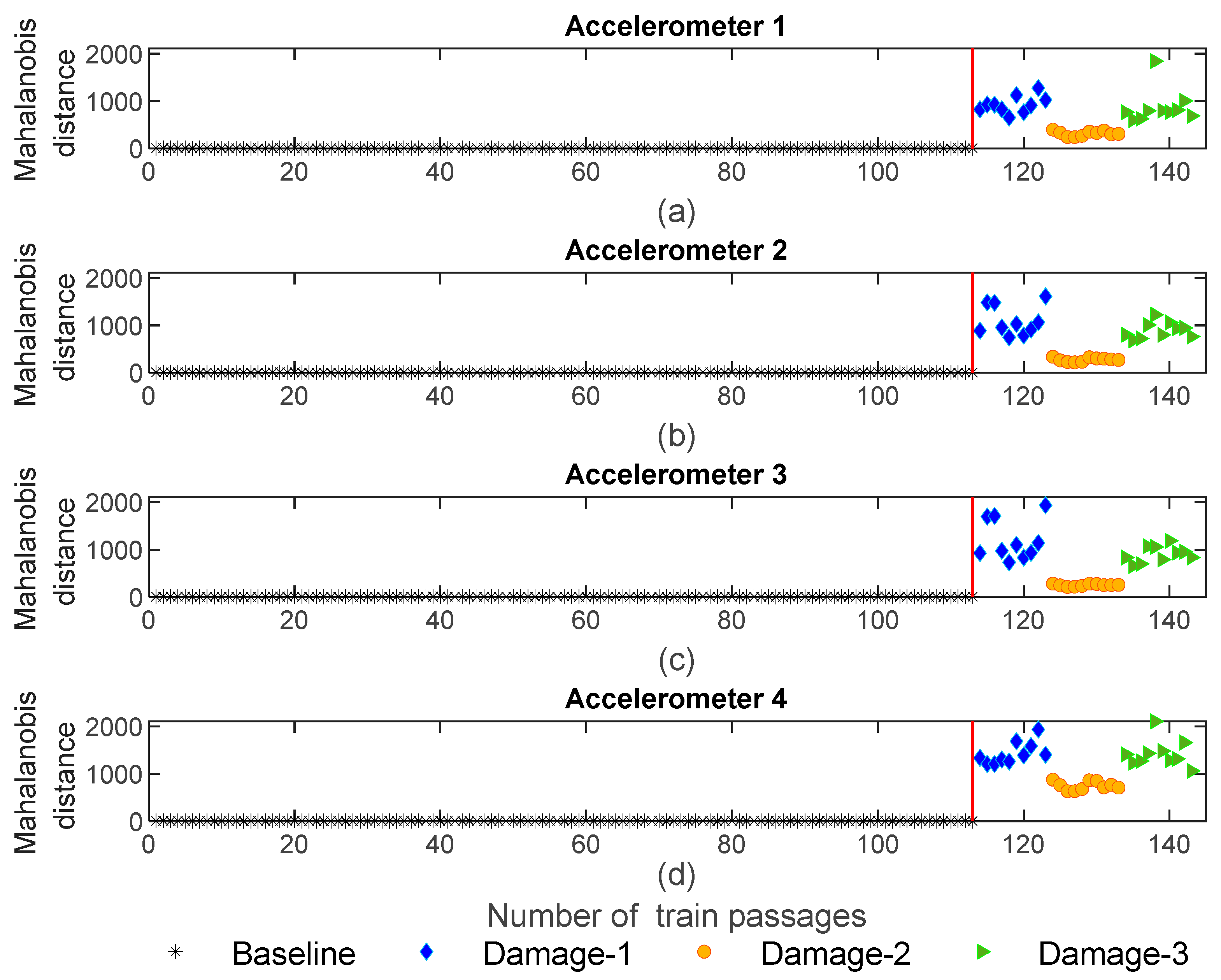
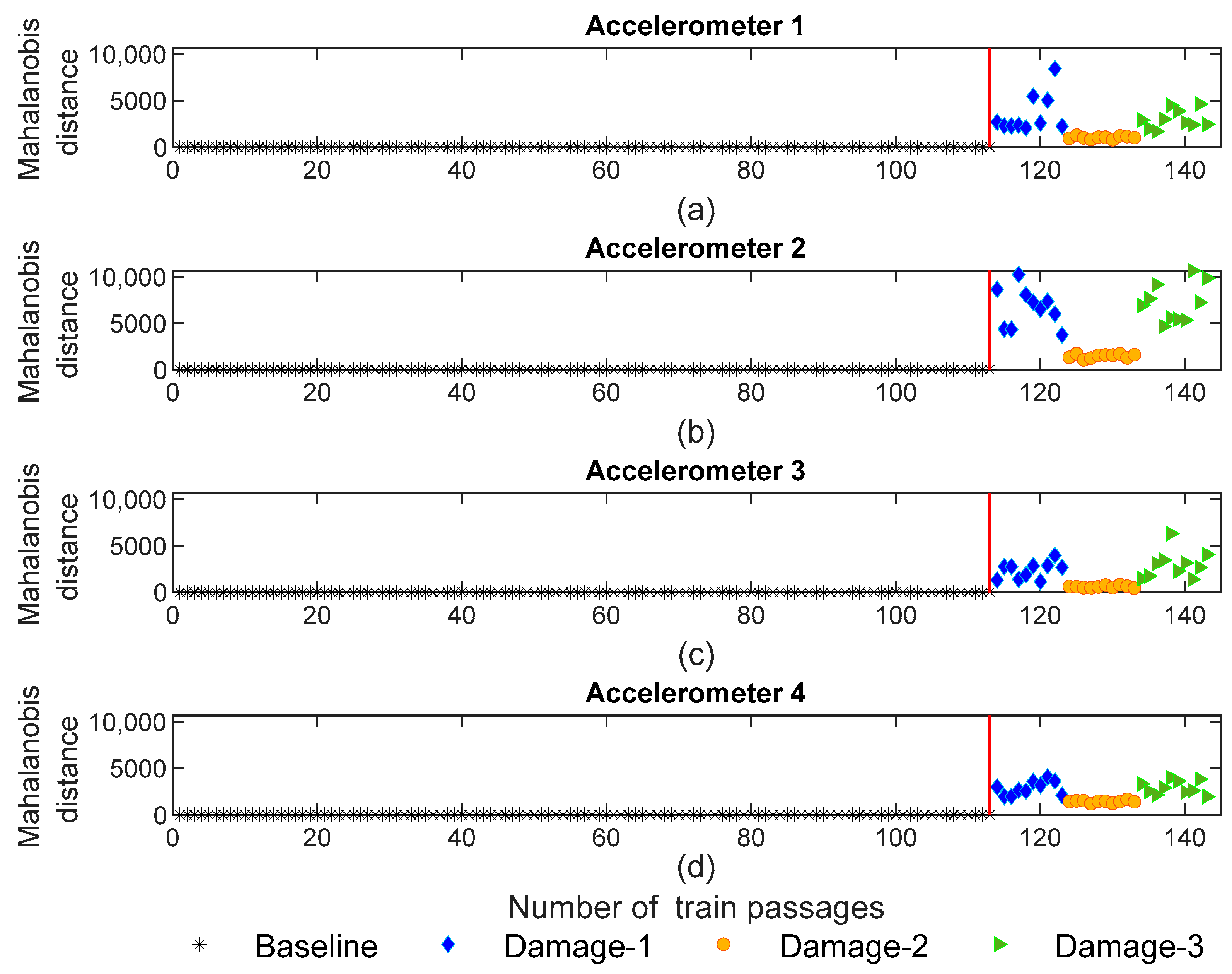
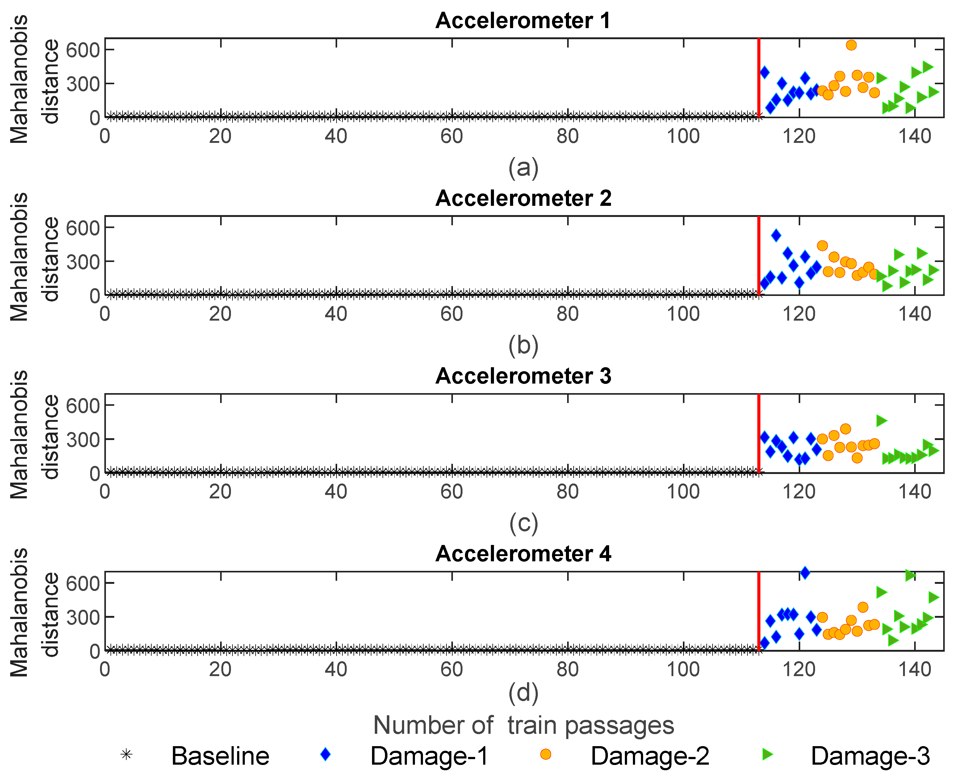
- Data fusion: implementation of a Mahalanobis distance (MD) to merge the features derived from each sensor and detect wheel defects more effectively. In the first stage, the features from each sensor are merged and, in the second stage, the multi-sensor information is fused to enhance the sensibility to the damage [26,32];
- Outlier analyses: upon completion of the previous step, a damage indicator (DI) is generated for each train passage; to distinguish each DI into a defective or a healthy wheel a statistical-based approach is used, in particular, an inverse cumulative distribution function that allows estimating a statistical confidence boundary (CB).
4. Application of the Methodology of Wheel Flat Detection to a Freight Train
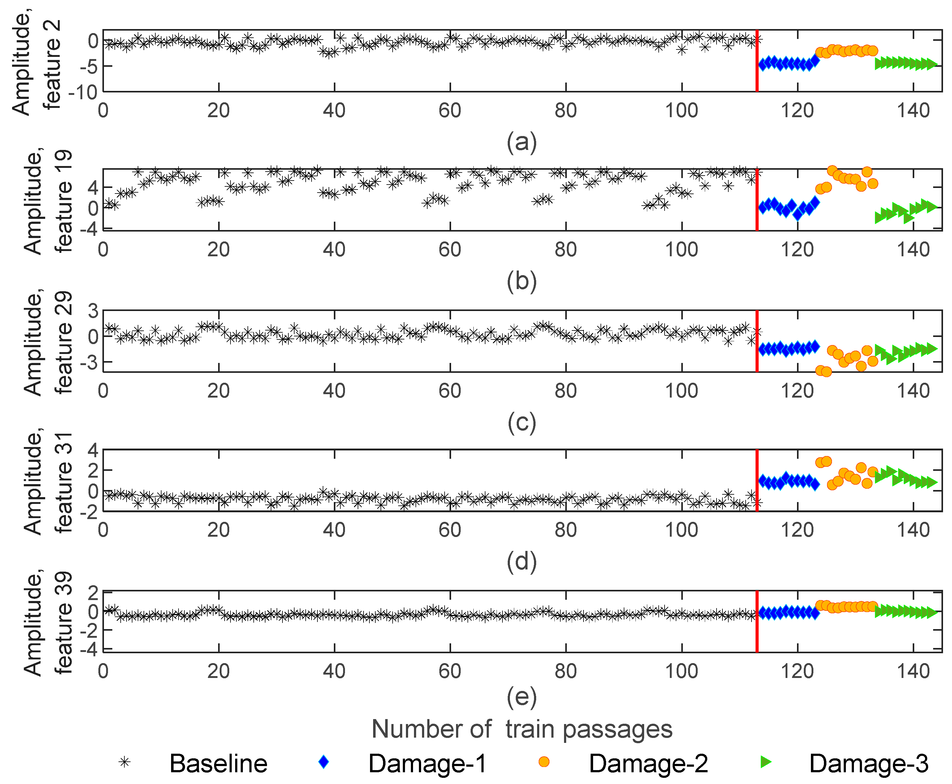
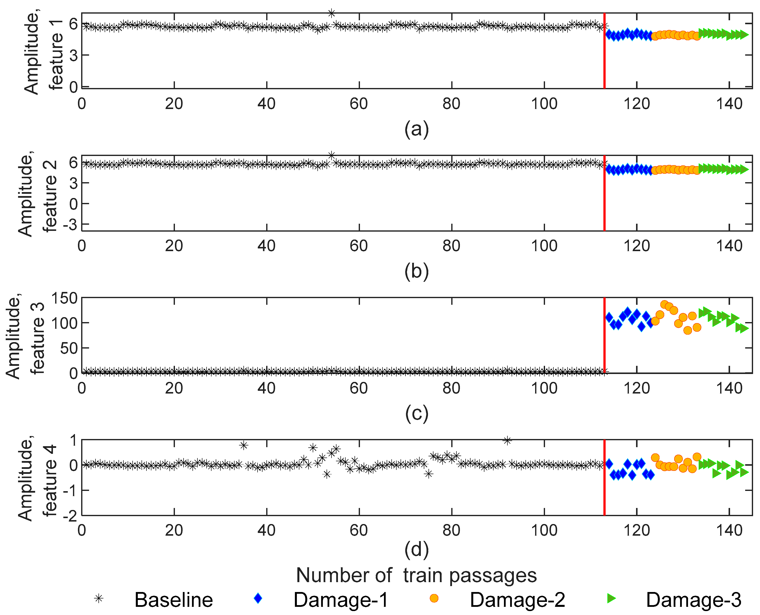
4.1. Feature Extraction
4.1.1. AR Model
4.1.2. ARX Model
4.1.3. CWT
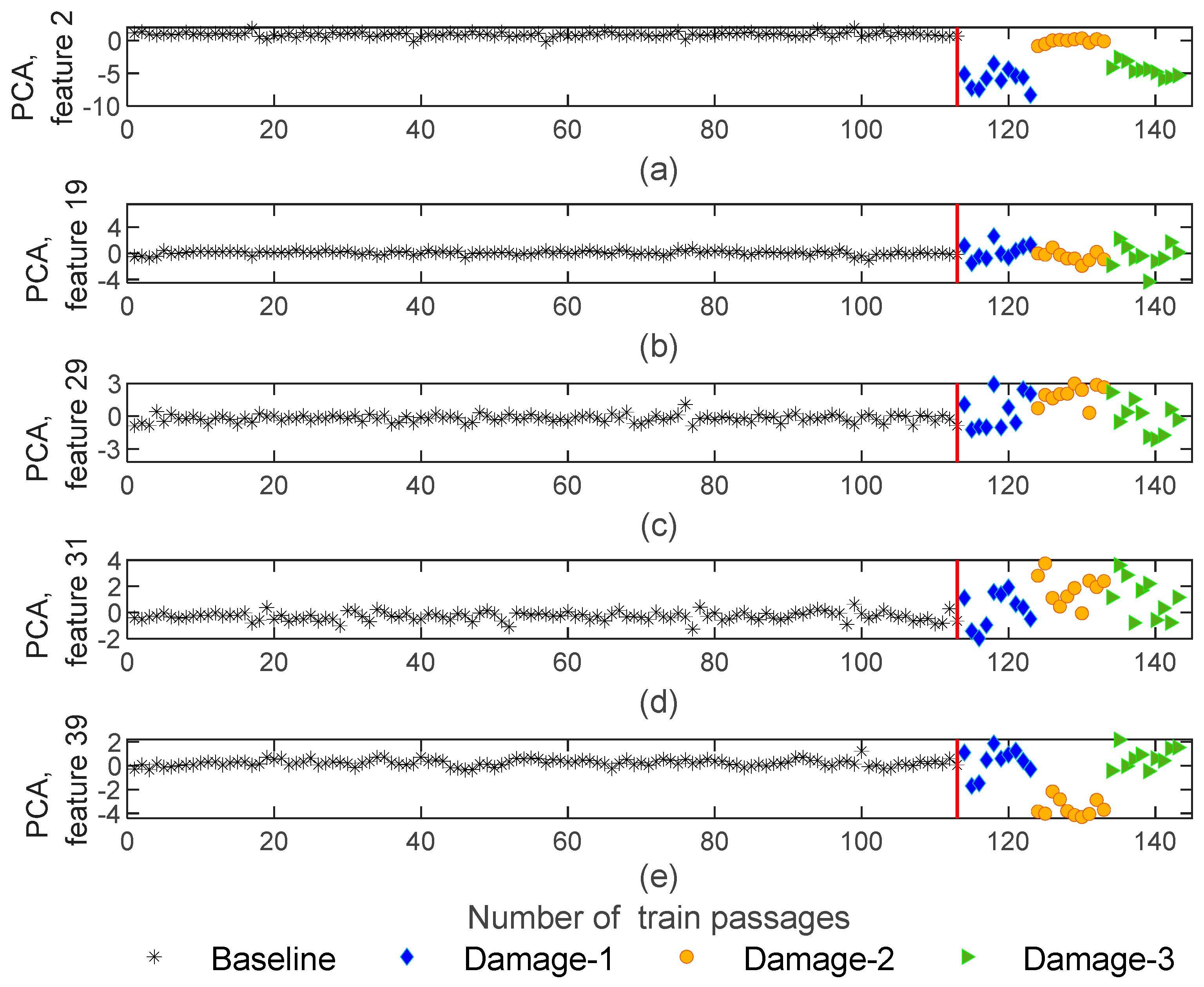
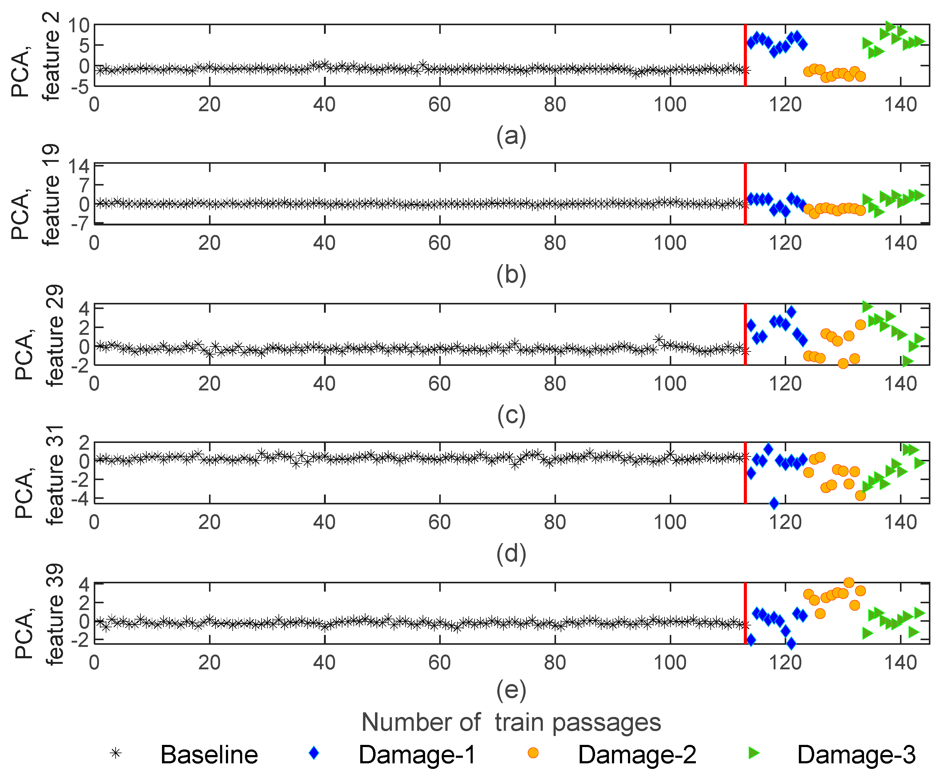
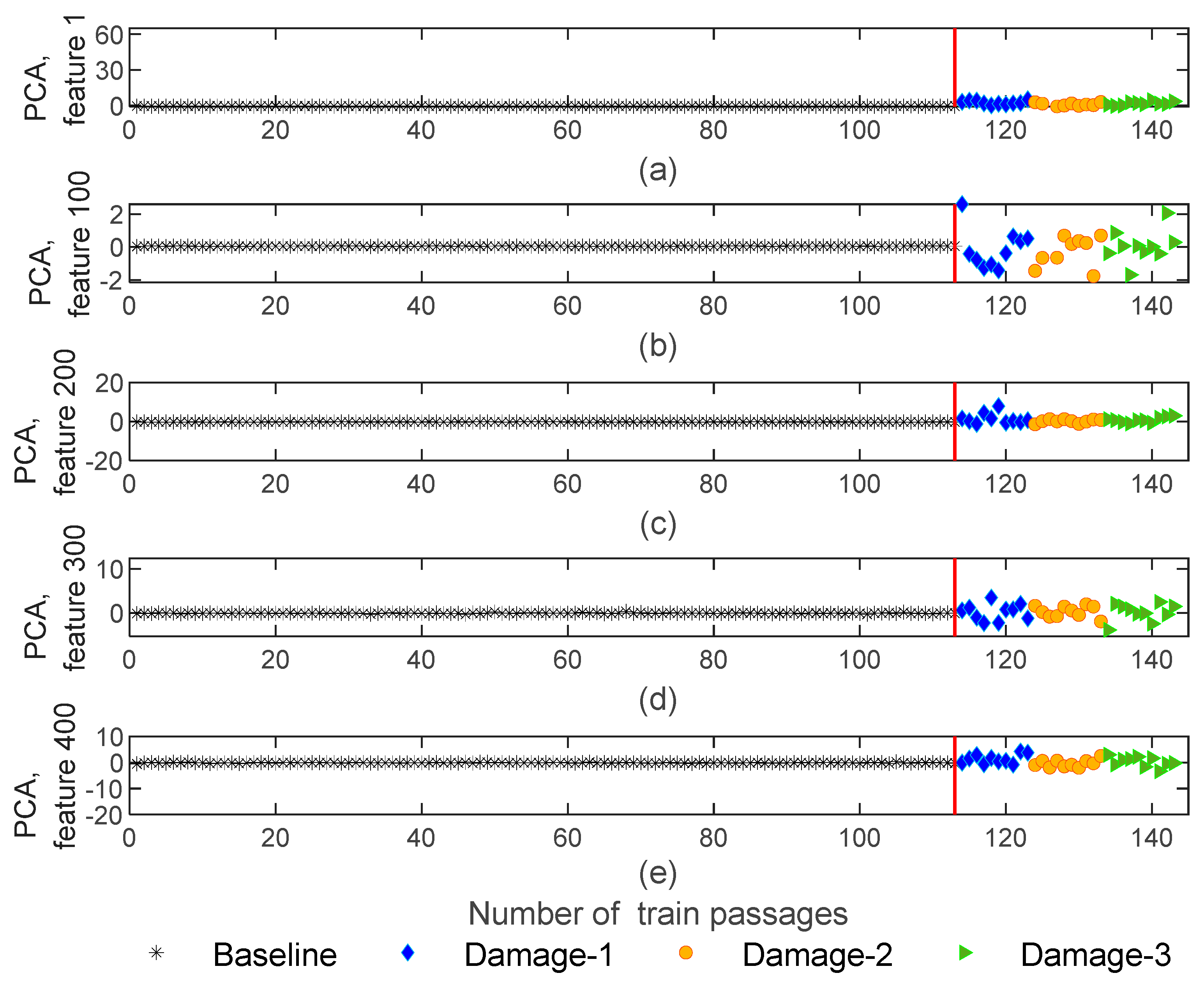
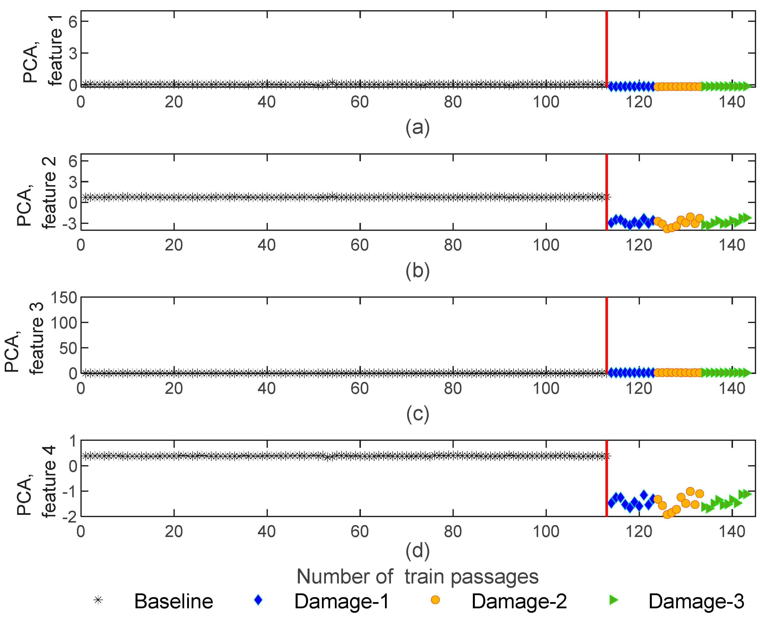
4.1.4. PCA
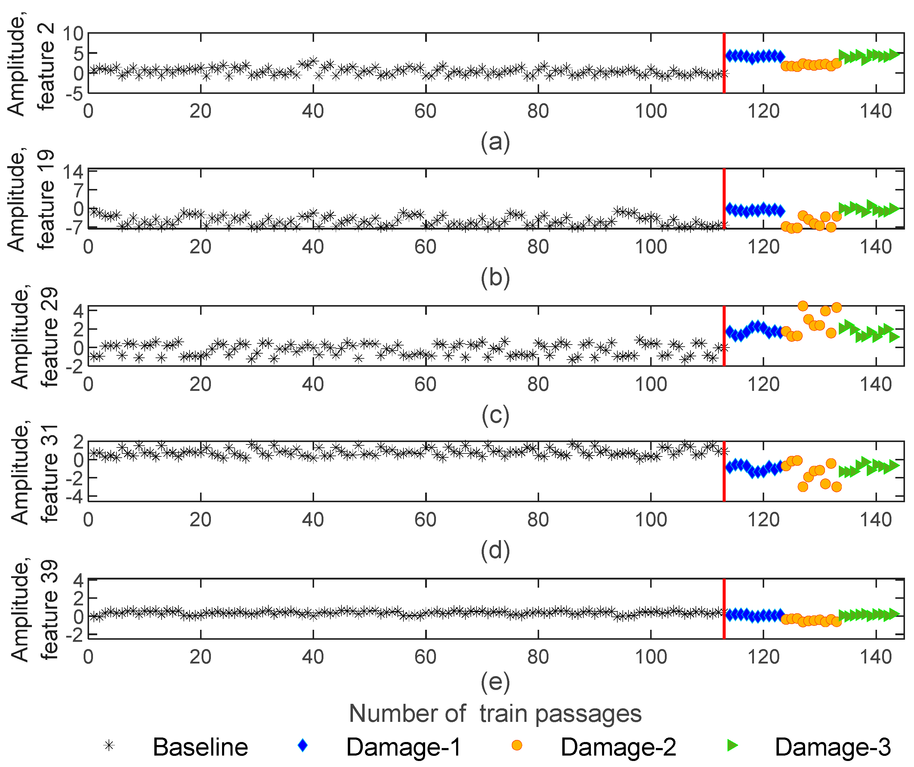
4.2. Feature Normalization
4.2.1. AR Model
4.2.2. ARX Model
4.2.3. CWT
4.2.4. PCA
4.3. Data Fusion
4.3.1. AR Model
4.3.2. ARX Model
4.3.3. CWT
4.3.4. PCA
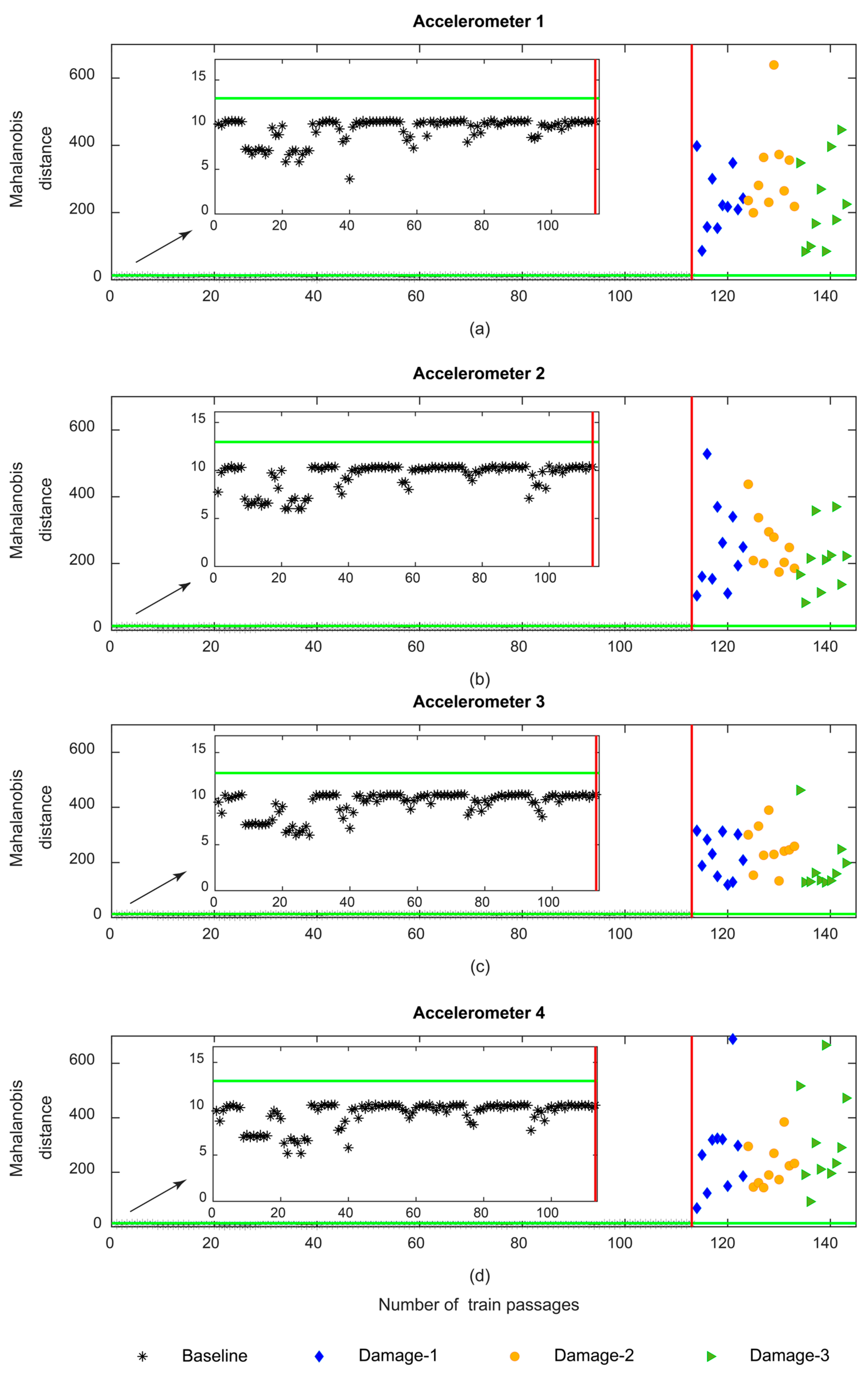
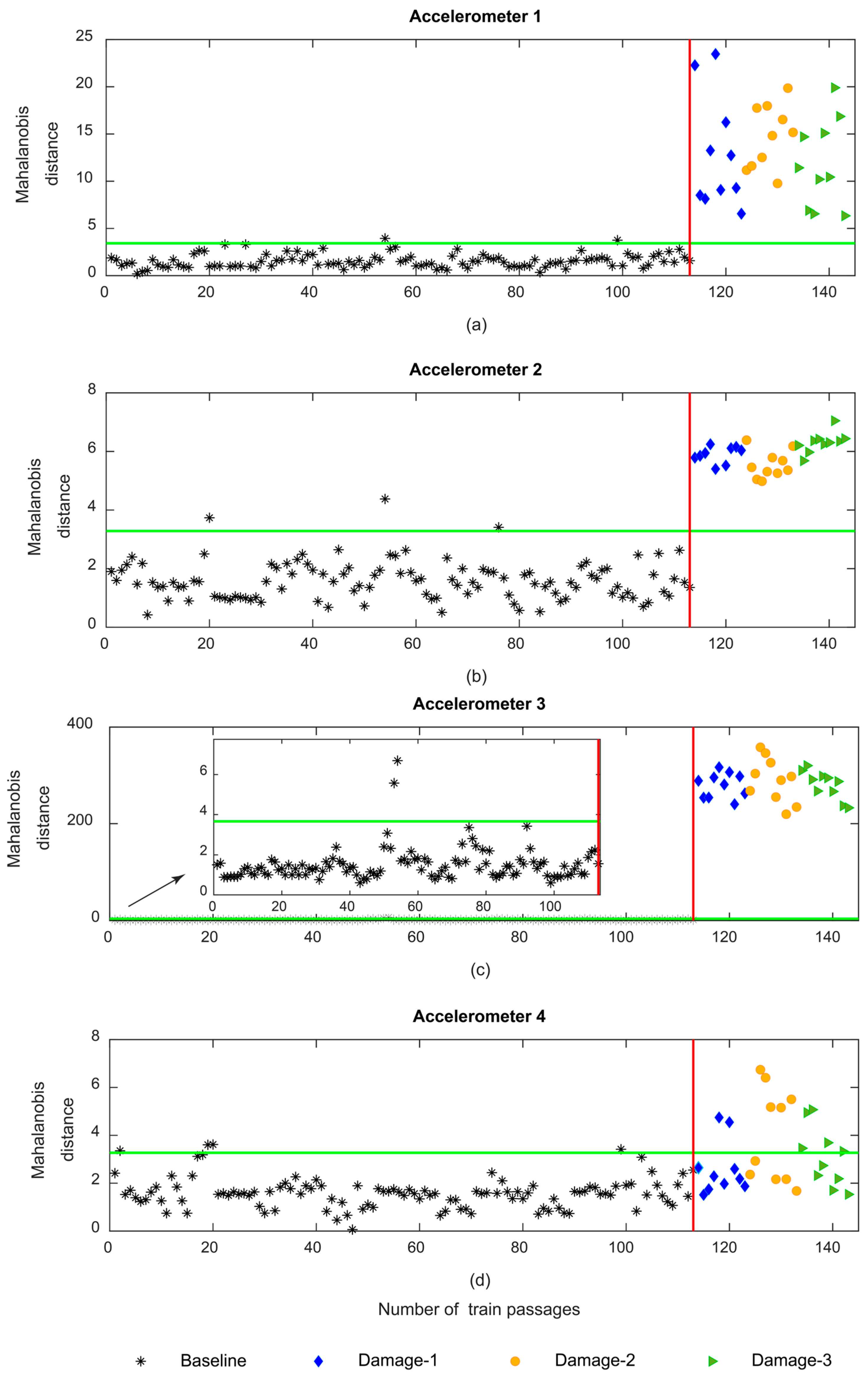
4.4. Outlier Analysis
4.4.1. AR Model
4.4.2. ARX Model
4.4.3. CWT
4.4.4. PCA
5. Conclusions
- the AR and ARX methods are the most accurate feature extraction methods for wheel flat damage detection as they can robustly detect defects; these two methods are sensitive to the side of the damage being the most promising to automatically distinguish an existing defective wheel on the right side from the left side in future works;
- the CWT method is only capable of detecting damaged wheels and is not sensitive to the side of the defect;
- the accuracy of the PCA method to detect the defective wheel is low and damage detection using this method lacks reliability;
- the ARX method is the only method that can robustly detect the wheel flat with accelerometers placed in the sleepers.
- One of the novelties of this research in relation to previous works [5,8] is the comparison of the accuracy of four different feature extraction techniques using an unsupervised learning methodology to automatically detect a defective wheel, which is a clear step forward in terms of the effectiveness of the proposed method, and allows full implementation for real-world applications.
Author Contributions
Funding
Institutional Review Board Statement
Informed Consent Statement
Data Availability Statement
Acknowledgments
Conflicts of Interest
References
- Meixedo, A.; Santos, J.; Ribeiro, D.; Calçada, R.; Todd, M. Damage detection in railway bridges using traffic-induced dy-namic responses. Eng. Struct. 2021, 238, 112189. [Google Scholar] [CrossRef]
- Mohammadi, M.; Mosleh, A.; Razzaghi, M.; Alves Costa, P.; Calçada, R. Stochastic analysis of railway embankment with uncer-tain soil parameters using polynomial chaos expansion. Struct. Infrastruct. Eng. 2022, 1–20. [Google Scholar] [CrossRef]
- Pintão, B.; Mosleh, A.; Vale, C.; Montenegro, P.; Costa, P. Development and Validation of a Weigh-in-Motion Methodology for Railway Tracks. Sensors 2022, 22, 1976. [Google Scholar] [CrossRef] [PubMed]
- Barke, D.W.; Chiu, W.K. A Review of the Effects of Out-Of-Round Wheels on Track and Vehicle Components. Proc. Inst. Mech. Eng. Part F J. Rail Rapid Transit 2005, 219, 151–175. [Google Scholar] [CrossRef]
- Mosleh, A.; Meixedo, A.; Ribeiro, D.; Montenegro, P.; Calçada, R. Automatic clustering-based approach for train wheels condition monitoring. Int. J. Rail Transp. 2022, 1–26. [Google Scholar] [CrossRef]
- Vale, C. Wheel Flats in the Dynamic Behavior of Ballasted and Slab Railway Tracks. Appl. Sci. 2021, 11, 7127. [Google Scholar]
- General Contract of Use for Wagons—GCU, Edition dated 1 January 2021. Available online: https://gcubureau.org/wp-content/uploads/Contract/2021/20210101_GCU_EN_full_version.pdf (accessed on 29 December 2022).
- Mosleh, A.; Meixedo, A.; Ribeiro, D.; Montenegro, P.; Calçada, R. Early wheel flat detection: An automatic data-driven wavelet-based approach for railways. Veh. Syst. Dyn. 2022, 1–30. [Google Scholar] [CrossRef]
- Nielsen, J.C.O.; Johansson, A. Out-of-round railway wheels-a literature survey. Proc. Inst. Mech. Eng. Part F J. Rail Rapid Transit 2000, 214, 79–91. [Google Scholar] [CrossRef]
- Bosso, N.; Gugliotta, A.; Zampieri, N. Wheel flat detection algorithm for onboard diagnostic. Measurement 2018, 123, 193–202. [Google Scholar] [CrossRef]
- Cavuto, A.; Martarelli, M.; Pandarese, G.; Revel, G.; Tomasini, E. Train wheel diagnostics by laser ultrasonics. Measurement 2016, 80, 99–107. [Google Scholar] [CrossRef]
- Alexandrou, G.; Kouroussis, G.; Verlinden, O. A comprehensive prediction model for vehicle/track/soil dynamic response due to wheel flats. Proc. Inst. Mech. Eng. Part F J. Rail Rapid Transit 2016, 230, 1088–1104. [Google Scholar]
- Amini, A.; Entezami, M.; Huang, Z.; Rowshandel, H.; Papaelias, M. Wayside detection of faults in railway axle bearings using time spectral kurtosis analysis on high-frequency acoustic emission signals. Adv. Mech. Eng. 2016, 8, 1687814016676000. [Google Scholar] [CrossRef] [Green Version]
- Mosleh, A.; Costa, P.A.; Calçada, R. A new strategy to estimate static loads for the dynamic weighing in motion of railway vehicles. Proc. Inst. Mech. Eng. Part F J. Rail Rapid Transit 2019, 234, 183–200. [Google Scholar] [CrossRef]
- Jiang, H.; Lin, J. Fault diagnosis of wheel flat using empirical mode decomposition-Hilbert envelope spectrum. Math. Probl. Eng. 2018, 2018, 8909031 . [Google Scholar] [CrossRef]
- Mosleh, A.; Montenegro, P.A.; Costa, P.A.; Calçada, R. Railway Vehicle Wheel Flat Detection with Multiple Records Using Spectral Kurtosis Analysis. Appl. Sci. 2021, 11, 4002. [Google Scholar] [CrossRef]
- Krummenacher, G.; Ong, C.S.; Koller, S.; Kobayashi, S.; Buhmann, J.M. Wheel Defect Detection with Machine Learning. IEEE Trans. Intell. Transp. Syst. 2018, 19, 1176–1187. [Google Scholar] [CrossRef]
- Ni, Y.-Q.; Zhang, Q.-H. A Bayesian machine learning approach for online detection of railway wheel defects using track-side monitoring. Struct. Health Monit. 2020, 20, 1536–1550. [Google Scholar] [CrossRef]
- Meixedo, A.; Santos, J.; Ribeiro, D.; Calçada, R.; Todd, M.D. Online unsupervised detection of structural changes using train–induced dynamic responses. Mech. Syst. Signal Process. 2022, 165, 108268. [Google Scholar] [CrossRef]
- Alves, V.; Meixedo, A.; Ribeiro, D.; Calçada, R.; Cury, A. Evaluation of the performance of different damage indicators in railway bridges. Procedia Eng. 2015, 114, 746–753. [Google Scholar]
- Javed, K.; Gouriveau, R.; Zerhouni, N.; Nectoux, P. Enabling Health Monitoring Approach Based on Vibration Data for Accurate Prognostics. IEEE Trans. Ind. Electron. 2015, 62, 647–656. [Google Scholar] [CrossRef]
- Shin, S.; Yun, C.B.; Futura, H.; Popovics, J.S. Nondestructive evaluation of crack depth in concrete using PCA-compressed wave transmission function and neural networks. Exp. Mech. 2008, 48, 225–231. [Google Scholar]
- Yan, A.M.; Kerschen, G.; De Boe, P.; Golinval, J.C. Structural damage diagnosis under varying environmental conditions—Part I: A linear analysis. Mech. Syst. Signal Process. 2005, 19, 847–864. [Google Scholar]
- Oh, C.K.; Sohn, H.; Bae, I.-H. Statistical novelty detection within the Yeongjong suspension bridge under environmental and operational variations. Smart Mater. Struct. 2009, 18, 125022. [Google Scholar]
- Figueiredo, E.; Cross, E. Linear approaches to modeling nonlinearities in long-term monitoring of bridges. J. Civ. Struct. Health Monit. 2013, 3, 187–194. [Google Scholar]
- Figueiredo, E.; Park, G.; Farrar, C.R.; Worden, K.; Figueiras, J. Machine learning algorithms for damage detection under operational and environmental variability. Struct. Health Monit. 2010, 10, 559–572. [Google Scholar] [CrossRef]
- Qian, L.; Zhang, L.; Bao, X.; Li, F.; Yang, J. Supervised sparse neighbourhood preserving embedding. IET Image Process. 2017, 11, 190–199. [Google Scholar] [CrossRef]
- Liu, Y.; Shi, Y.; Mu, F.; Cheng, J.; Li, C.; Chen, X. Multimodal MRI volumetric data fusion with convolutional neural networks. IEEE Trans. Instrum. Meas. 2022, 71, 1–15. [Google Scholar]
- Pan, Y.; Sun, Y.; Li, Z.; Gardoni, P. Machine learning approaches to estimate suspension parameters for performance degradation assessment using accurate dynamic simulations. Reliab. Eng. Syst. Saf. 2022, 230, 108950. [Google Scholar]
- Kontolati, K.; Loukrezis, D.; dos Santos, K.R.; Giovanis, D.G.; Shields, M.D. Manifold learning-based polynomial chaos expansions for high-dimensional surrogate models. Int. J. Uncertain. Quantif. 2022, 12, 39–64. [Google Scholar] [CrossRef]
- Wang, J.; Xie, J.; Zhao, R.; Zhang, L.; Duan, L. Multisensory fusion based virtual tool wear sensing for ubiquitous manufacturing. Robot. Comput. Integr. Manuf. 2017, 45, 47–58. [Google Scholar] [CrossRef]
- Bull, L.A.; Worden, K.; Fuentes, R.; Manson, G.; Cross, E.J.; Dervilis, N. Outlier ensembles: A robust method for damage detection and unsupervised feature extraction from high-dimensional data. J. Sound Vib. 2019, 453, 126–150. [Google Scholar]
- Li, Y.; Zuo, M.J.; Lin, J.; Liu, J. Fault detection method for railway wheel flat using an adaptive multiscale morphological filter. Mech. Syst. Signal Process. 2017, 84, 642–658. [Google Scholar] [CrossRef]
- Nick, W.; Asamene, K.; Bullock, G.; Esterline, A.; Sundaresan, M. A study of machine learning techniques for detecting and classifying structural damage. Int. J. Mach. Learn. Comput. 2015, 5, 313. [Google Scholar] [CrossRef]
- Addin, O.; Sapuan, S.M.; Mahdi, E.; Othman, M. A Naïve-Bayes classifier for damage detection in engineering materials. Mater. Des. 2007, 28, 2379–2386. [Google Scholar] [CrossRef]
- Vitola, J.; Pozo, F.; Tibaduiza, D.A.; Anaya, M. Distributed Piezoelectric Sensor System for Damage Identification in Structures Subjected to Temperature Changes. Sensors 2017, 17, 1252. [Google Scholar] [CrossRef]
- Montenegro, P.A.; Neves, S.G.M.; Calçada, R.; Tanabe, M.; Sogabe, M. Wheel–rail contact formulation for analyzing the lateral train–structure dynamic interaction. Comput. Struct. 2015, 152, 200–214. [Google Scholar]
- Hertz, H. Ueber die Berührung fester elastischer Körper. J. Für Die Reine Und Angew. Math. 1882, 92, 156–171. [Google Scholar] [CrossRef]
- Kalker, J.J. Book of Tables for the Herzian Creep-force Law; Faculty of Technical Mathematics and Informatics, Delft University of Technology: Delft, The Netherlands, 1996. [Google Scholar]
- MATLAB®, version R2022a; The MathWorks Inc.: Natick, MA, USA, 2022.
- ANSYS®; Release 19.2; Academic Research: Canonsburg, PA, USA, 2018.
- Mosleh, A.; Montenegro, P.; Alves Costa, P.; Calçada, R. An approach for wheel flat detection of railway train wheels using envelope spectrum analysis. Struct. Infrastruct. Eng. 2021, 17, 1710–1729. [Google Scholar] [CrossRef]
- Mosleh, A.; Montenegro, P.A.; Costa, P.A.; Calçada, R. Approaches for weigh-in-motion and wheel defect detection of railway vehicles. In Rail Infrastructure Resilience; Elsevier: Amsterdam, The Netherlands, 2022; pp. 183–207. [Google Scholar]
- UIC. Code of Practice for the Loading and Securing of Goods on Railway Wagons; UIC: Paris, France, 2022. [Google Scholar]
- Meixedo, A.; Ribeiro, D.; Santos, J.; Calçada, R.; Todd, M.D. Real-Time Unsupervised Detection of Early Damage in Railway Bridges Using Traffic-Induced Responses. In Structural Health Monitoring Based on Data Science Techniques; Springer: Berlin/Heidelberg, Germany, 2022; pp. 117–142. [Google Scholar]
- Tomé, E.S.; Pimentel, M.; Figueiras, J. Damage detection under environmental and operational effects using cointegration analysis–application to experimental data from a cable-stayed bridge. Mech. Syst. Signal Process. 2020, 135, 106386. [Google Scholar]


| Baseline Scenarios | Damaged Scenarios | |
|---|---|---|
| Train | Freight—Laagrss wagon | |
| Number of loading schemes | 6 | 1 (full capacity) |
| Unevenness profiles | 4 | 1 |
| Speeds (km/h) | 40–120 | 80 |
| Noise ratio | 5% | |
| Flat lengths (mm) | − | 50–100 |
| Number of numerical analyses | 100 | 30 |
Disclaimer/Publisher’s Note: The statements, opinions and data contained in all publications are solely those of the individual author(s) and contributor(s) and not of MDPI and/or the editor(s). MDPI and/or the editor(s) disclaim responsibility for any injury to people or property resulting from any ideas, methods, instructions or products referred to in the content. |
© 2023 by the authors. Licensee MDPI, Basel, Switzerland. This article is an open access article distributed under the terms and conditions of the Creative Commons Attribution (CC BY) license (https://creativecommons.org/licenses/by/4.0/).
Share and Cite
Mohammadi, M.; Mosleh, A.; Vale, C.; Ribeiro, D.; Montenegro, P.; Meixedo, A. An Unsupervised Learning Approach for Wayside Train Wheel Flat Detection. Sensors 2023, 23, 1910. https://doi.org/10.3390/s23041910
Mohammadi M, Mosleh A, Vale C, Ribeiro D, Montenegro P, Meixedo A. An Unsupervised Learning Approach for Wayside Train Wheel Flat Detection. Sensors. 2023; 23(4):1910. https://doi.org/10.3390/s23041910
Chicago/Turabian StyleMohammadi, Mohammadreza, Araliya Mosleh, Cecilia Vale, Diogo Ribeiro, Pedro Montenegro, and Andreia Meixedo. 2023. "An Unsupervised Learning Approach for Wayside Train Wheel Flat Detection" Sensors 23, no. 4: 1910. https://doi.org/10.3390/s23041910