
“In the Wild” Video Content as a Special Case of User Generated Content and a System for Its Recognition

Abstract
:1. Introduction
1.1. Research Scope
- Present motivation on what the problem is and why it is important (addressed in Section 1);
- Show our objectives (addressed in Section 1.1);
- Reveal gaps in the literature (addressed in Section 1.2);
- Propose to fill some of these gaps (addressed in Section 1.3);
- Present overview on our overall approach (addressed in Section 2);
- Show results contributing to the literature and to the video analysis research area in general (addressed in Section 3);
- Discuss novelties of the paper (addressed in Section 4).
1.2. Related Work for Multimedia Quality Assessment
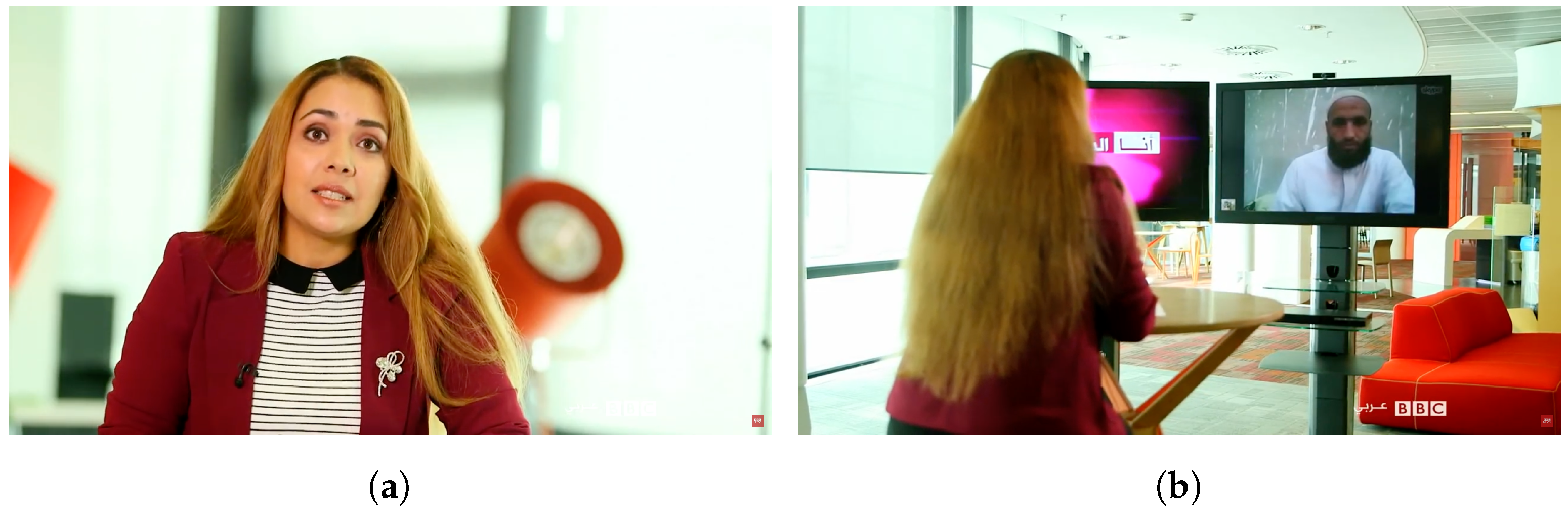
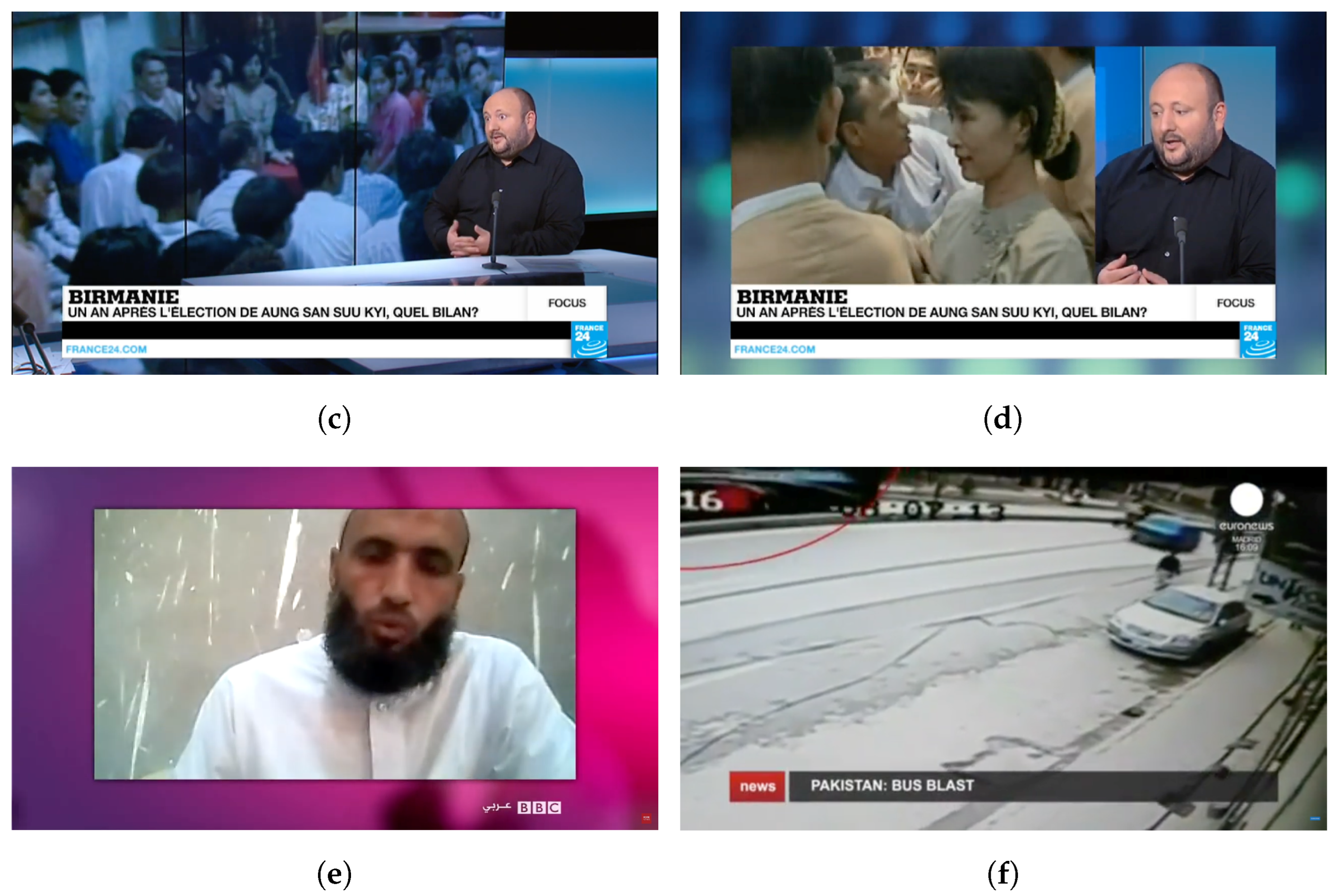
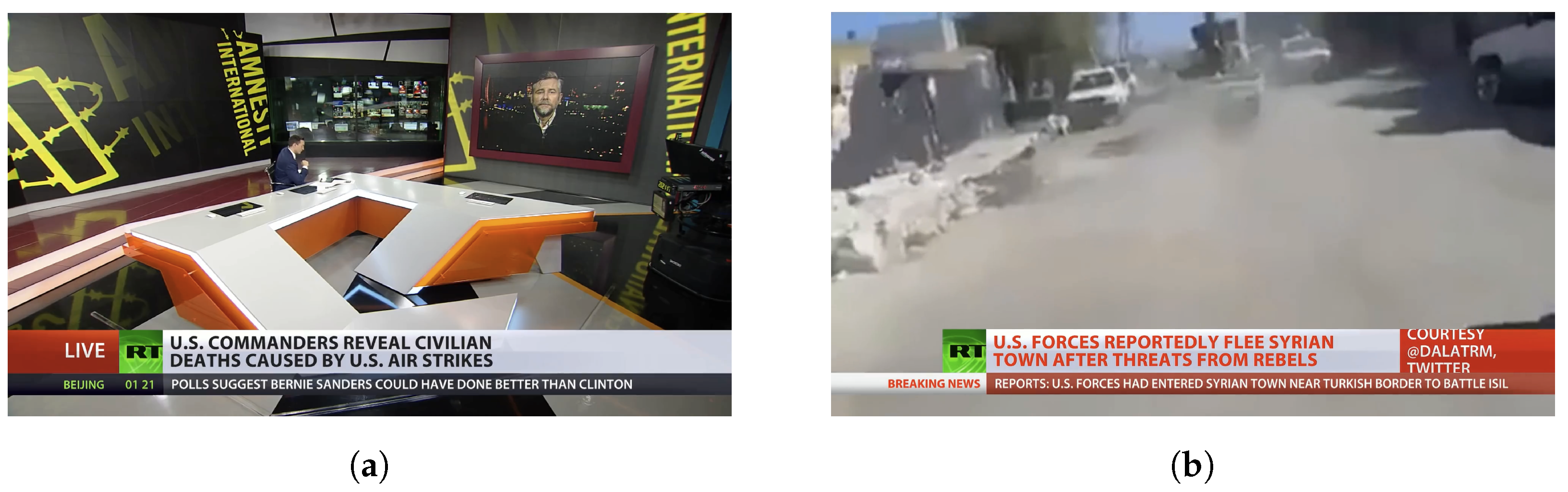
1.3. “In the Wild” Definition
- They are recorded without the use of professional equipment. In particular without using a professional camera to produce videos.
- They are not recorded in a studio. In other words, they are captured in an environment without an intentional lighting setup.
- They are shot without a gimbal or similar image stabilization equipment. In short, these are handheld videos.
- They are not subjected to significant post-processing aimed at intentionally improving their quality. In other words, they are not post-processed at the film production level.
2. Materials and Methods
2.1. Database Construction
- Professional video sequences are those recorded in a film studio or outside using professional equipment with image stabilization. These video sequences are also often post-processed.
- “In the wild” video sequences can best be described as being recorded and processed under natural conditions.
2.2. Database Description
2.3. Video Indicators
2.4. Model
2.4.1. Algorithm
2.4.2. Description of Modeling and Parameters Used
- “max_depth”
- “scale_pos_weight”
- “learning_rate”
- “reg_lambda”
- “colsample_bytree”
- “gamma”
2.4.3. Determination of Hyperparameters
- “max_depth”: 10
- “scale_pos_weight”: 0.6
- “learning_rate”: 0.12
- “reg_lambda”: 0.7
- “colsample_bytree”: 0.7
- “gamma”: 0.3
2.4.4. Model Training
3. Results
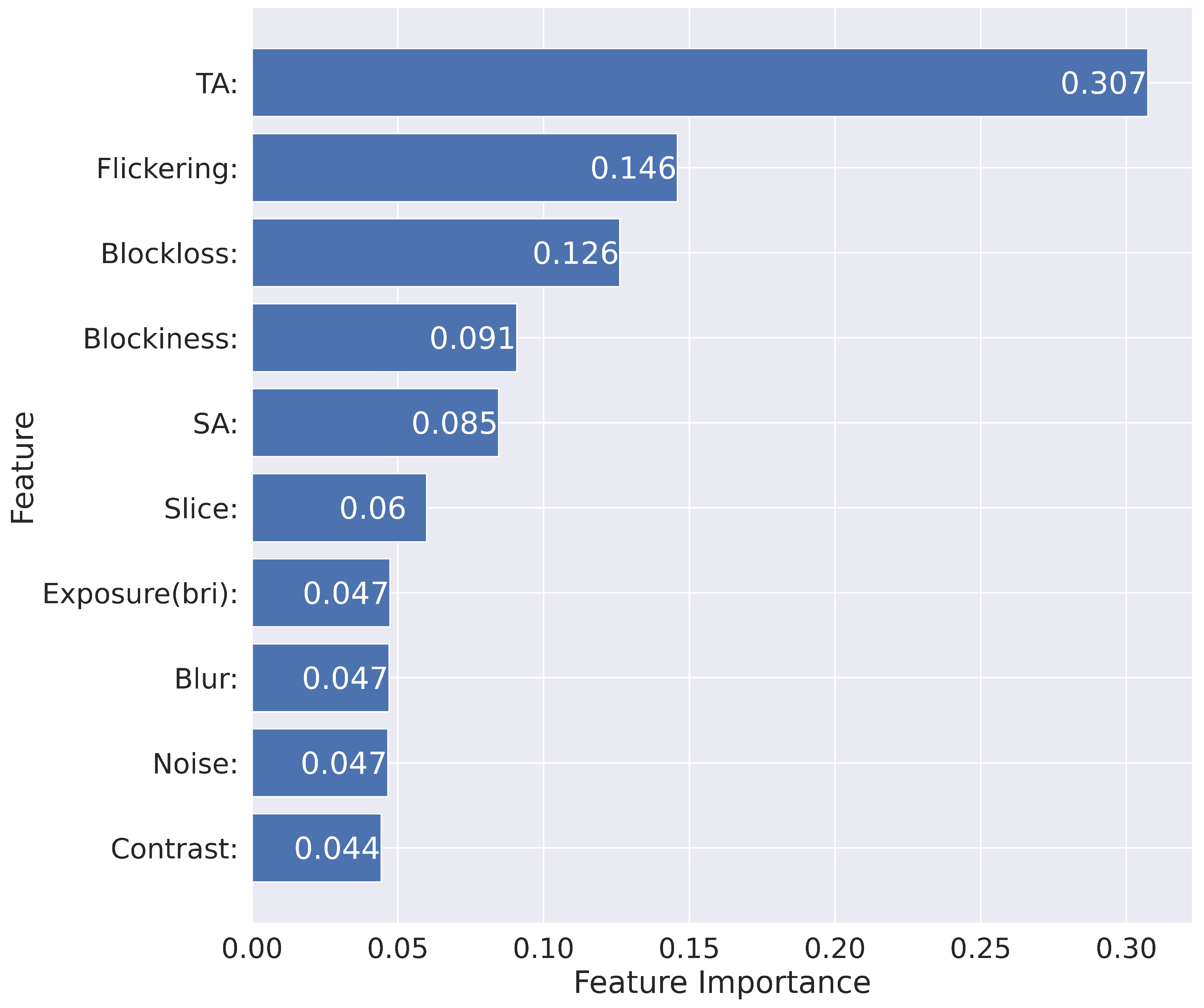
- “In the wild” samples are more difficult to classify.
- The indicators responsible for the errors are as follows. Temporal Activity Block Loss Spatial Activity Slicing Blur and Noise.
- The two most relevant indicators that cause errors were Temporal Activity and Block Loss.
4. Discussion
Supplementary Materials
Author Contributions
Funding
Institutional Review Board Statement
Informed Consent Statement
Data Availability Statement
Acknowledgments
Conflicts of Interest
Appendix A


| Professional | “In the wild” | |
|---|---|---|
| Temporal Activity (TA) | 4.244378042 | 25.96020345 |
| Flickering | −0.787083846 | −0.789469515 |
| Blockloss | 1.648851049 | 2.119697212 |
| Blockiness | 0.956104266 | 0.845652727 |
| Spatial Activity (SA) | 104.2437722 | 70.60911164 |
| Slice | 53.46148252 | 102.3170606 |
| Exposure (brightness) | 125.9440559 | 128.6848485 |
| Blur | 4.102888112 | 3.672139394 |
| Noise | 0.334337063 | 0.321036364 |
| Contrast | 62.00859979 | 43.41147194 |
Appendix B
- $ python −m agh_vqis ./my_video.mp4 −u
- from agh_vqis import process_single_mm_file
- from pathlib import Path
- process_single_mm_file(Path(‘my_video.mp4’), options = {
- ‘ugc’: True
- })
References
- Cisco. Cisco Annual Internet Report (2018–2023) White Paper; Cisco: San Jose, CA, USA, 2020. [Google Scholar]
- Berthon, P.; Pitt, L.; Kietzmann, J.; McCarthy, I.P. CGIP: Managing consumer-generated intellectual property. Calif. Manag. Rev. 2015, 57, 43–62. [Google Scholar] [CrossRef]
- Krumm, J.; Davies, N.; Narayanaswami, C. User-generated content. IEEE Pervasive Comput. 2008, 7, 10–11. [Google Scholar] [CrossRef]
- Zhao, K.; Zhang, P.; Lee, H.M. Understanding the impacts of user-and marketer-generated content on free digital content consumption. Decis. Support Syst. 2022, 154, 113684. [Google Scholar] [CrossRef]
- Zhang, M. Swiss TV Station Replaces Cameras with iPhones and Selfie Sticks. Downloaded Oct. 2015, 1, 2015. [Google Scholar]
- Leszczuk, M.; Janowski, L.; Nawała, J.; Grega, M. User-Generated Content (UGC)/In-The-Wild Video Content Recognition. In Proceedings of the Asian Conference on Intelligent Information and Database Systems, Ho Chi Minh City, Vietnam, 28–30 November 2022; Springer: Cham, Switzerland, 2022; pp. 356–368. [Google Scholar]
- Karadimce, A.; Davcev, D.P. Towards Improved Model for User Satisfaction Assessment of Multimedia Cloud Services. J. Mob. Multimed. 2018, 157–196. [Google Scholar] [CrossRef]
- Li, D.; Jiang, T.; Jiang, M. Quality assessment of in-the-wild videos. In Proceedings of the 27th ACM International Conference on Multimedia (MM ’19), Nice, France, 21–25 October 2019; pp. 2351–2359. [Google Scholar]
- Ying, Z.; Mandal, M.; Ghadiyaram, D.; Bovik, A. Patch-VQ: ‘Patching Up’ the Video Quality Problem. In Proceedings of the IEEE/CVF Conference on Computer Vision and Pattern Recognition (CVPR), Nashville, TN, USA, 20–25 June 2021; pp. 14019–14029. [Google Scholar]
- Tu, Z.; Chen, C.J.; Wang, Y.; Birkbeck, N.; Adsumilli, B.; Bovik, A.C. Video Quality Assessment of User Generated Content: A Benchmark Study and a New Model. In Proceedings of the 2021 IEEE International Conference on Image Processing (ICIP), Anchorage, AK, USA, 19–22 September 2021; IEEE: Piscataway Township, MJ, USA, 2021; pp. 1409–1413. [Google Scholar] [CrossRef]
- Yi, F.; Chen, M.; Sun, W.; Min, X.; Tian, Y.; Zhai, G. Attention Based Network For No-Reference UGC Video Quality Assessment. In Proceedings of the 2021 IEEE International Conference on Image Processing (ICIP), Anchorage, AK, USA, 19–22 September 2021; IEEE: Piscataway Township, MJ, USA, 2021; pp. 1414–1418. [Google Scholar] [CrossRef]
- Marc Egger, A.; Schoder, D. Who Are We Listening To? Detecting User-Generated Content (Ugc) on the Web. In Proceedings of the European Conference on Information Systems (ECIS 2015), Münster, Germany, 26–29 May 2015. [Google Scholar]
- Guo, J.; Gurrin, C.; Lao, S. Who produced this video, amateur or professional? In Proceedings of the 3rd ACM Conference on INTERNATIONAL Conference on Multimedia Retrieval, Dallas, TX, USA, 16–20 April 2013; pp. 271–278. [Google Scholar]
- Guo, J.; Gurrin, C. Short user-generated videos classification using accompanied audio categories. In Proceedings of the 2012 ACM International Workshop on Audio and Multimedia Methods for Large-Scale Video Analysis, Lisboa, Portugal, 14 October 2012; pp. 15–20. [Google Scholar]
- Leszczuk, M.; Hanusiak, M.; Farias, M.C.Q.; Wyckens, E.; Heston, G. Recent developments in visual quality monitoring by key performance indicators. Multimed. Tools Appl. 2016, 75, 10745–10767. [Google Scholar] [CrossRef]
- Nawała, J.; Leszczuk, M.; Zajdel, M.; Baran, R. Software package for measurement of quality indicators working in no-reference model. Multimed. Tools Appl. 2016, 1–7. [Google Scholar] [CrossRef]
- Romaniak, P.; Janowski, L.; Leszczuk, M.; Papir, Z. Perceptual quality assessment for H.264/AVC compression. In Proceedings of the 2012 IEEE Consumer Communications and Networking Conference (CCNC), Las Vegas, NV, USA, 14–17 January 2012; pp. 597–602. [Google Scholar] [CrossRef]
- Mu, M.; Romaniak, P.; Mauthe, A.; Leszczuk, M.; Janowski, L.; Cerqueira, E. Framework for the integrated video quality assessment. Multimed. Tools Appl. 2012, 61, 787–817. [Google Scholar] [CrossRef]
- Leszczuk, M. Assessing Task-Based Video Quality—A Journey from Subjective Psycho-Physical Experiments to Objective Quality Models. In Proceedings of the Multimedia Communications, Services and Security; Dziech, A., Czyżewski, A., Eds.; Springer: Berlin/Heidelberg, Germany, 2011; pp. 91–99. [Google Scholar]
- Janowski, L.; Papir, Z. Modeling subjective tests of quality of experience with a Generalized Linear Model. In Proceedings of the 2009 International Workshop on Quality of Multimedia Experience, Lippstadt, Germany, 5–7 September 2009; pp. 35–40. [Google Scholar] [CrossRef]
- Chen, T.; Guestrin, C. Xgboost: A scalable tree boosting system. In Proceedings of the 22nd Acm Sigkdd International Conference on Knowledge Discovery and Data Mining, San Francisco, CA, USA, 13–17 August 2016; pp. 785–794. [Google Scholar]
- Guarino, A.; Lettieri, N.; Malandrino, D.; Zaccagnino, R.; Capo, C. Adam or Eve? Automatic users’ gender classification via gestures analysis on touch devices. Neural Comput. Appl. 2022, 34, 18473–18495. [Google Scholar] [CrossRef]
- Xu, Z.; Hu, J.; Deng, W. Recurrent convolutional neural network for video classification. In Proceedings of the 2016 IEEE International Conference on Multimedia and Expo (ICME), Seattle, WA, USA, 11–15 July 2016; IEEE: Piscataway Township, NJ, USA, 2016; pp. 1–6. [Google Scholar]
- Seeland M, M.P. Multi-view classification with convolutional neural networks. PLoS ONE 2021, 16, e0245230. [Google Scholar] [CrossRef] [PubMed]
- Tejero-de Pablos, A.; Nakashima, Y.; Sato, T.; Yokoya, N.; Linna, M.; Rahtu, E. Summarization of user-generated sports video by using deep action recognition features. IEEE Trans. Multimed. 2018, 20, 2000–2011. [Google Scholar] [CrossRef]
- Psallidas, T.; Koromilas, P.; Giannakopoulos, T.; Spyrou, E. Multimodal summarization of user-generated videos. Appl. Sci. 2021, 11, 5260. [Google Scholar] [CrossRef]
- Nuutinen, M.; Virtanen, T.; Vaahteranoksa, M.; Vuori, T.; Oittinen, P.; Hakkinen, J. CVD2014—A Database for Evaluating No-Reference Video Quality Assessment Algorithms. IEEE Trans. Image Process. 2016, 25, 3073–3086. [Google Scholar] [CrossRef] [PubMed]
- Ghadiyaram, D.; Pan, J.; Bovik, A.C.; Moorthy, A.K.; Panda, P.; Yang, K.C. In-Capture Mobile Video Distortions: A Study of Subjective Behavior and Objective Algorithms. IEEE Trans. Circuits Syst. Video Technol. 2018, 28, 2061–2077. [Google Scholar] [CrossRef]
- Hosu, V.; Hahn, F.; Jenadeleh, M.; Lin, H.; Men, H.; Szirányi, T.; Li, S.; Saupe, D. The Konstanz natural video database (KoNViD-1k). In Proceedings of the 2017 Ninth International Conference on Quality of Multimedia Experience (QoMEX), Erfurt, Germany, 31 May–2 June 2017; pp. 1–6. [Google Scholar]
- Pinson, M.H.; Boyd, K.S.; Hooker, J.; Muntean, K. How to choose video sequences for video quality assessment. In Proceedings of the Seventh International Workshop on Video Processing and Quality Metrics for Consumer Electronics (VPQM-2013), Scottsdale, AZ, USA, 30 January–1 February 2013; pp. 79–85. [Google Scholar]
- Badiola, A.; Zorrilla, A.M.; Garcia-Zapirain Soto, B.; Grega, M.; Leszczuk, M.; Smaïli, K. Evaluation of Improved Components of AMIS Project for Speech Recognition, Machine Translation and Video/Audio/Text Summarization. In Proceedings of the International Conference on Multimedia Communications, Services and Security, Kraków, Poland, 8–9 October 2020; Springer: Cham, Switzerland, 2020; pp. 320–331. [Google Scholar]


| Format | Number of Samples |
|---|---|
| 144p | 2512 |
| 360p | 98 |
| 480p | 310 |
| 720p | 7893 |
| 1080p | 1254 |
| # | Name | Description |
|---|---|---|
| 1 | Blockiness [17] | Block boundary artefacts, also known as checker-boarding, quilting, or macro-blocking |
| 2 | Spatial Activity (SA) [17] | The degree of detail in a video, such as the presence of sharp edges, minute details, and textures |
| 3 | Block Loss [15] | A vision artefact resulting in the loss of selected image blocks |
| 4 | Blur [17,18] | Loss of high spatial frequency image detail, typically at sharp edges, as a result |
| 5 | Temporal Activity (TA) [17] | The amount of temporal change in a video sequence frames |
| 6 | Exposure (brightness) [19] | The amount of light reaching the surface of the electronic image sensor per unit area |
| 7 | Contrast | The disparity in shape, colour, and lighting that exists between several elements of an image |
| 8 | Noise [20] | Unpredictable changes in the brightness or colour of frames |
| 9 | Slicing [15] | A vision artefact resulting in the loss of selected image slices |
| 10 | Flickering [17] | Frequently fluctuating colour or brightness throughout the time dimension |
| Model Name | Average Value | Largest Value | Smallest Value | Standard Deviation |
|---|---|---|---|---|
| XGBClassifier (with tunable parameters) | 91.60% | 92.50% | 90.70% | 0.005 |
| XGBClassifier (default) | 89.90% | 91.10% | 88.80% | 0.006 |
| AdaBoostClassifier (default) | 89.50% | 90.80% | 88.40% | 0.007 |
| SVC (default) | 87.50% | 89.00% | 85.90% | 0.007 |
| LogisticRegression (default) | 88.20% | 89.50% | 87.00% | 0.006 |
| DecisionTreeClassifier (default) | 87.20% | 88.20% | 86.70% | 0.005 |
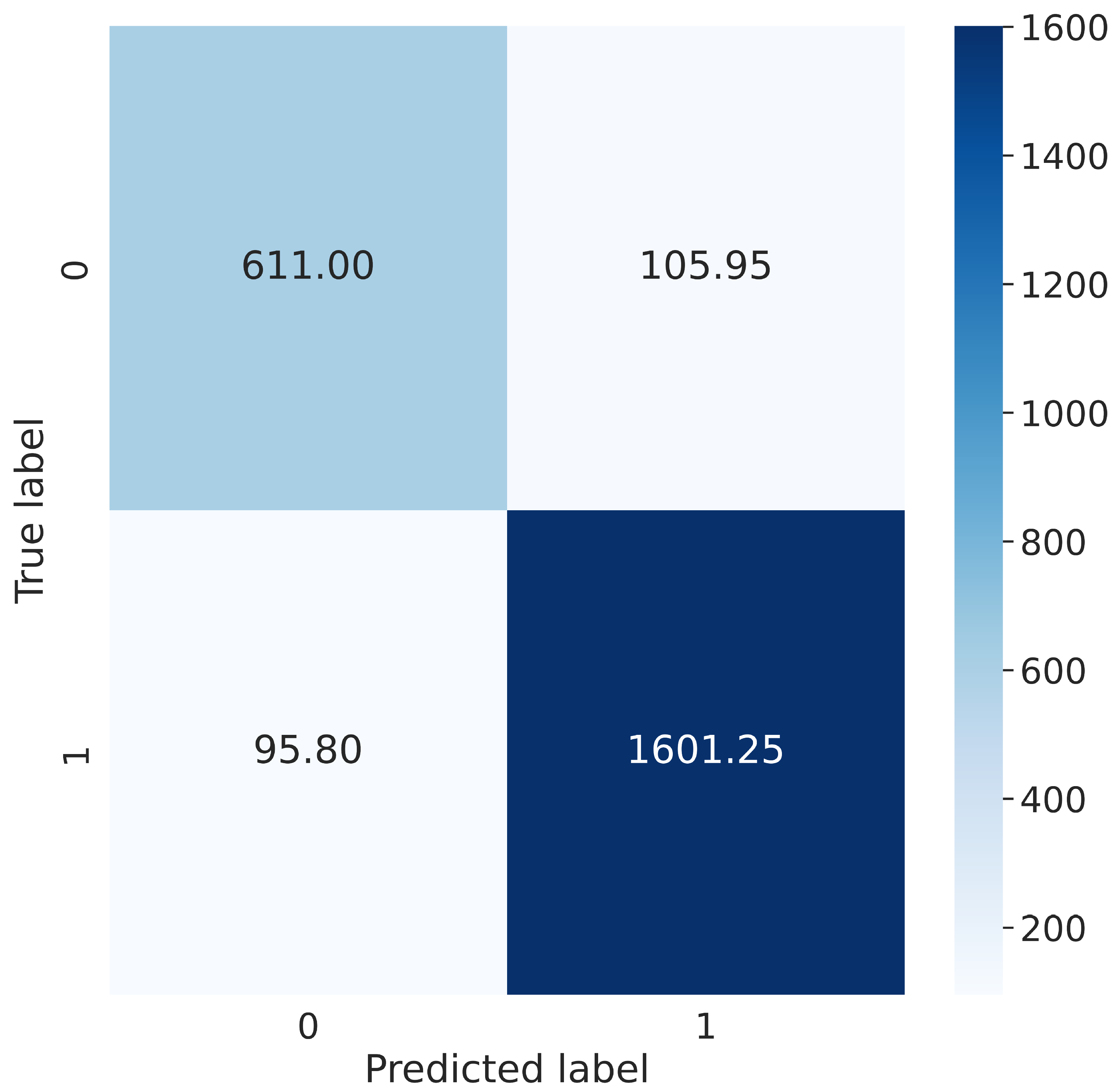
| Sample Category | Precision | Recall | F1-Score |
|---|---|---|---|
| “In the wild” Content | 0.8520 | 0.8655 | 0.8590 |
| Proffesionally Generated Content | 0.9445 | 0.9370 | 0.9395 |
| “In the Wild”Correct | “In the Wild”Wrong | PRO Correct | PRO Wrong | |
|---|---|---|---|---|
| Temporal Activity (TA) | 8.31% | 53.86% | 9.67% | 133.62% |
| Flickering | 0.24% | 1.89% | 0.14% | 1.57% |
| Blockloss | 2.15% | 40.89% | 8.92% | 161.58% |
| Blockiness | 0.86% | 8.56% | 0.52% | 8.10% |
| Spatial Activity (SA) | 2.00% | 9.89% | 1.92% | 36.75% |
| Slice | 4.21% | 103.72% | 4.27% | 80.48% |
| Exposure (brightness) | 0.43% | 0.74% | 0.28% | 2.01% |
| Blur | 0.43% | 3.14% | 3.09% | 46.71% |
| Noise | 4.74% | 43.92% | 2.97% | 65.56% |
| Contrast | 0.81% | 1.01% | 0.45% | 1.46% |
| Model Name | Accuracy | Precision | Recall | F1-Score |
|---|---|---|---|---|
| CNN | 89.60% | 92.16% | 93.30% | 0.93 |
| CNN-LSTM | 89.67% | 92.66% | 92.78% | 0.93 |
| Model Name | Precision | Recall | F1-Score |
|---|---|---|---|
| XGBClassifier (with tunable parameters) | 91.75% | 91.75% | 0.917 |
| XGBClassifier (default) | 90.00% | 90.00% | 0.9000 |
| AdaBoostClassifier (default) | 89.45% | 89.45% | 0.8945 |
| SVC (default) | 87.30% | 87.40% | 0.8705 |
| LogisticRegression (default) | 87.75% | 87.90% | 0.8775 |
| DecisionTreeClassifier (default) | 87.30% | 87.10% | 0.8715 |
Disclaimer/Publisher’s Note: The statements, opinions and data contained in all publications are solely those of the individual author(s) and contributor(s) and not of MDPI and/or the editor(s). MDPI and/or the editor(s) disclaim responsibility for any injury to people or property resulting from any ideas, methods, instructions or products referred to in the content. |
© 2023 by the authors. Licensee MDPI, Basel, Switzerland. This article is an open access article distributed under the terms and conditions of the Creative Commons Attribution (CC BY) license (https://creativecommons.org/licenses/by/4.0/).
Share and Cite
Leszczuk, M.; Kobosko, M.; Nawała, J.; Korus, F.; Grega, M. “In the Wild” Video Content as a Special Case of User Generated Content and a System for Its Recognition. Sensors 2023, 23, 1769. https://doi.org/10.3390/s23041769
Leszczuk M, Kobosko M, Nawała J, Korus F, Grega M. “In the Wild” Video Content as a Special Case of User Generated Content and a System for Its Recognition. Sensors. 2023; 23(4):1769. https://doi.org/10.3390/s23041769
Chicago/Turabian StyleLeszczuk, Mikołaj, Marek Kobosko, Jakub Nawała, Filip Korus, and Michał Grega. 2023. "“In the Wild” Video Content as a Special Case of User Generated Content and a System for Its Recognition" Sensors 23, no. 4: 1769. https://doi.org/10.3390/s23041769