

A Feature-Trajectory-Smoothed High-Speed Model for Video Anomaly Detection

Abstract
:1. Introduction
- A a video anomaly-detection model, namely, FTS-LSTM, is proposed. In this model, an FTS loss is designed to enable the LSTM layer to learn videos’ temporal regularity better.
- A new indicator to detect anomalies, namely, the FTS indicator, is proposed. It can detect anomalies precisely with a high speed.
- This work has good generalization capability and can easily transfer to other models with LSTM layers.
2. Related Work
2.1. Traditional Machine Learning Stage
2.2. Deep Learning Stage
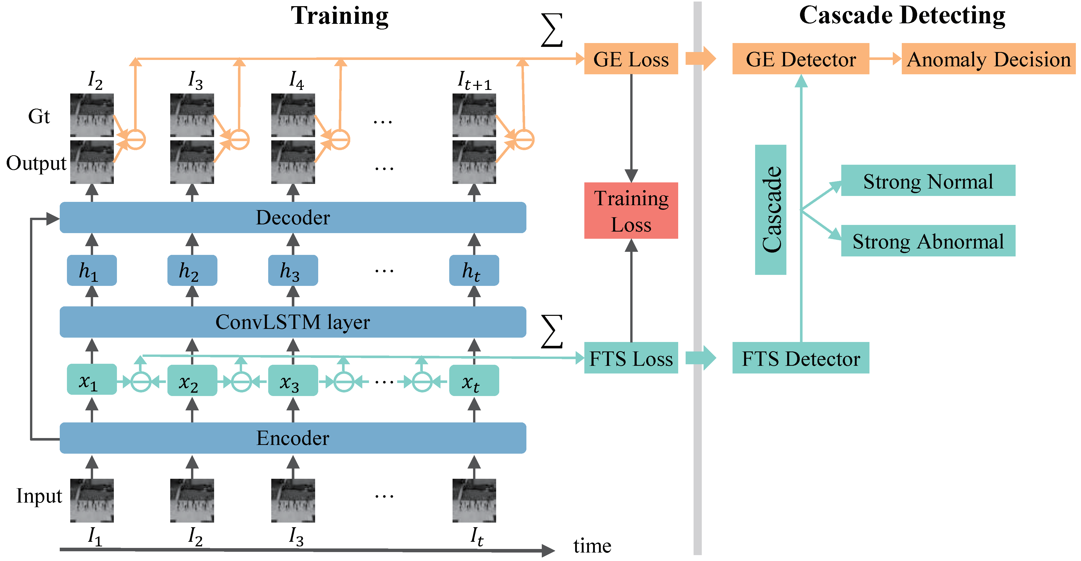
3. Method
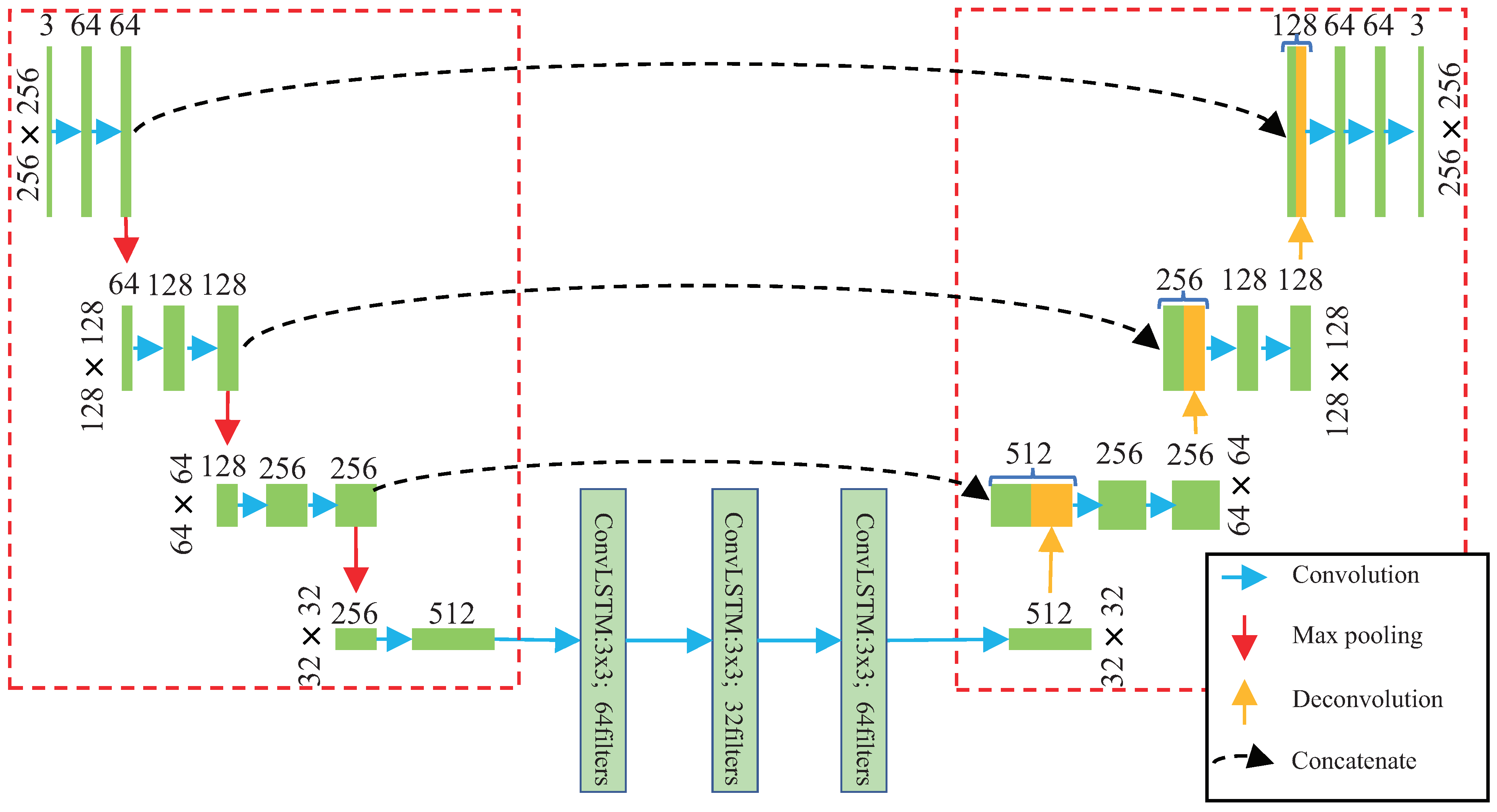
3.1. Network Structure

3.1.1. Encoder Module
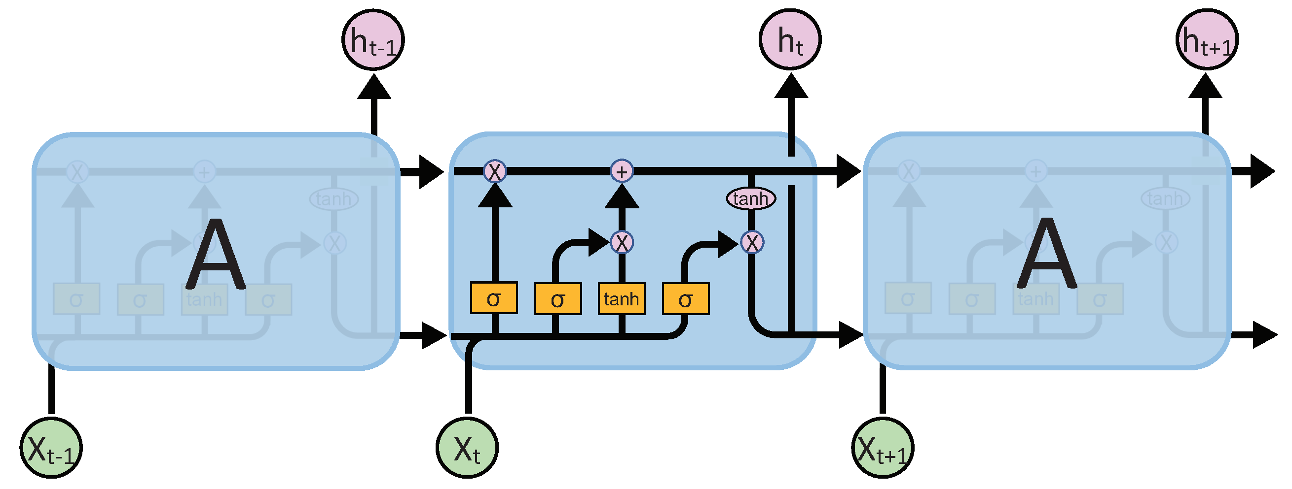
3.1.2. ConvLSTM Module
3.1.3. Decoder Module
3.2. The Training Process
3.2.1. The GE Loss
3.2.2. FTS Loss
3.2.3. Global Training Loss
3.3. Detecting Process
3.3.1. The GE Detector
3.3.2. The FTS Detector
3.3.3. Cascade
3.3.4. Discussion
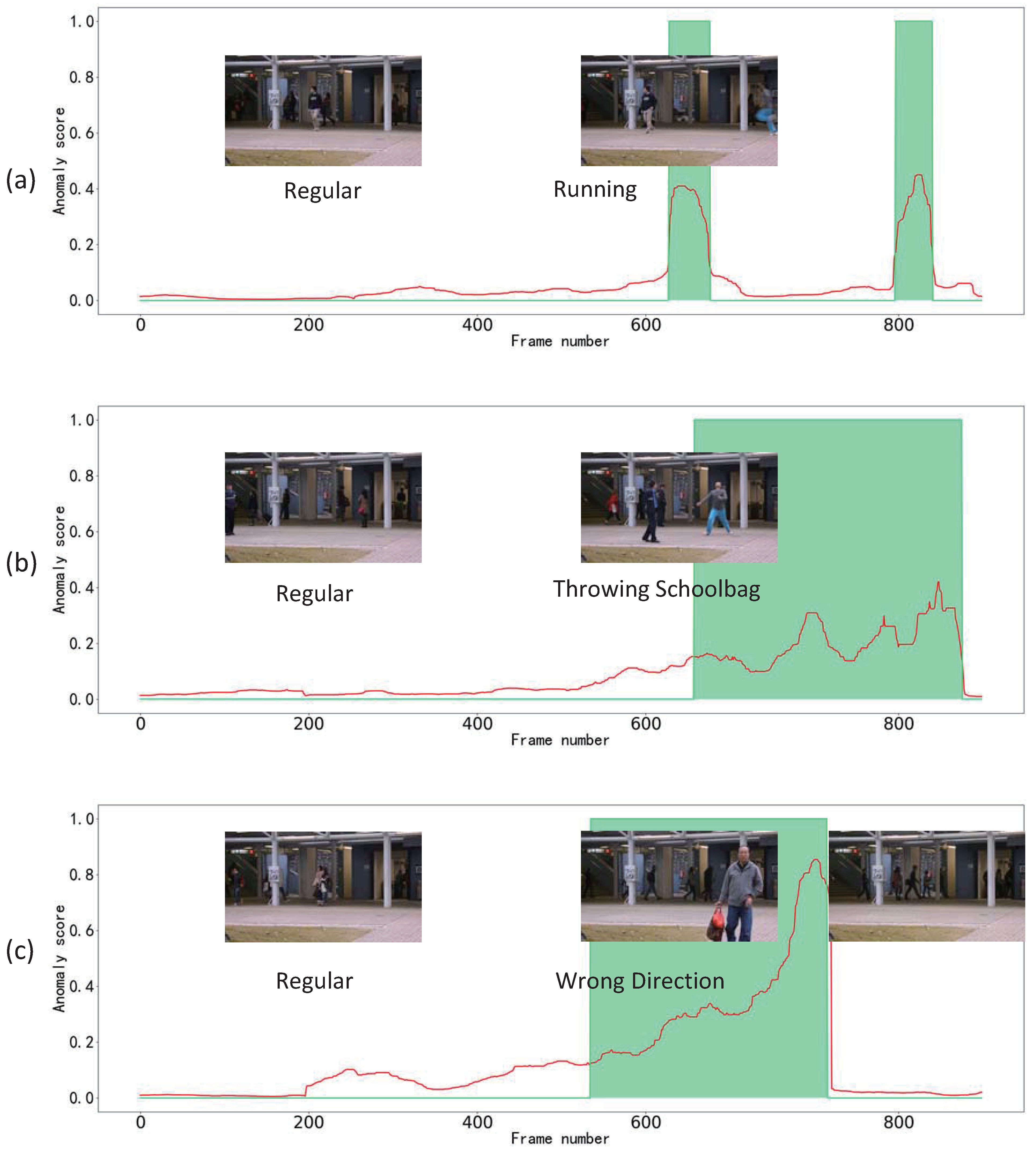
4. Results
4.1. Datasets
4.2. Implementation Details
4.3. Evaluation Metric
4.4. Anomaly-Detection Performances
4.5. Ablation Study
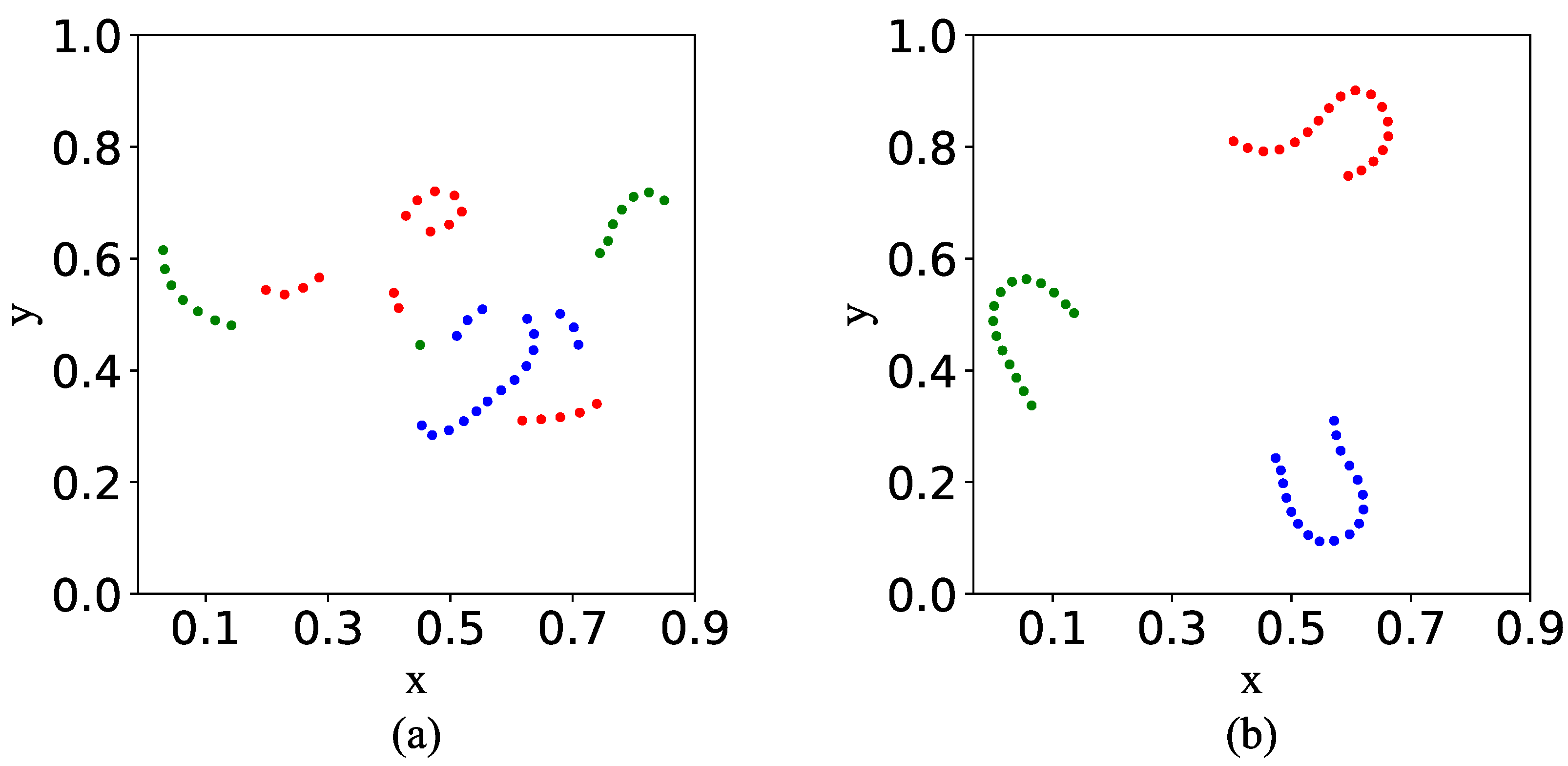
4.5.1. Feature Space TSNE Visualization

| Method | – | Ped1 | Ped2 | Avenue | SH | Speed |
|---|---|---|---|---|---|---|
| Deep Distance-based | DeepOC [14] | 83.5 | 96.9 | 86.6 | – | 40 FPS |
| Deep Probability-based | Tang et al. [20] | 84.7 | 96.3 | 85.1 | 71.5 | 30 FPS |
| Aggregation methods | STAN [21] | 82.1 | 96.5 | 87.2 | – | – |
| TAM-Net [22] | 83.5 | 98.1 | 78.3 | – | – | |
| MAAS [23] | 85.8 | 99.0 | 92.1 | 69.7 | 4 FPS | |
| Deep Generation-error-based | Unet [8] | 83.1 | 95.4 | 85.1 | 72.8 | 12 FPS |
| Ts-Unet [48] | – | 97.8 | 88.4 | – | 12 FPS | |
| sRNN [19] | – | 92.2 | 83.5 | 69.6 | 10 FPS | |
| MemAE [40] | – | 94.1 | 83.3 | 71.2 | 38 FPS | |
| Zhou et al. [41] | 83.9 | 96.0 | 86.0 | – | – | |
| FTS-LSTM (ours) | 83.5 | 98.3 | 91.1 | 72.9 | 117 FPS |


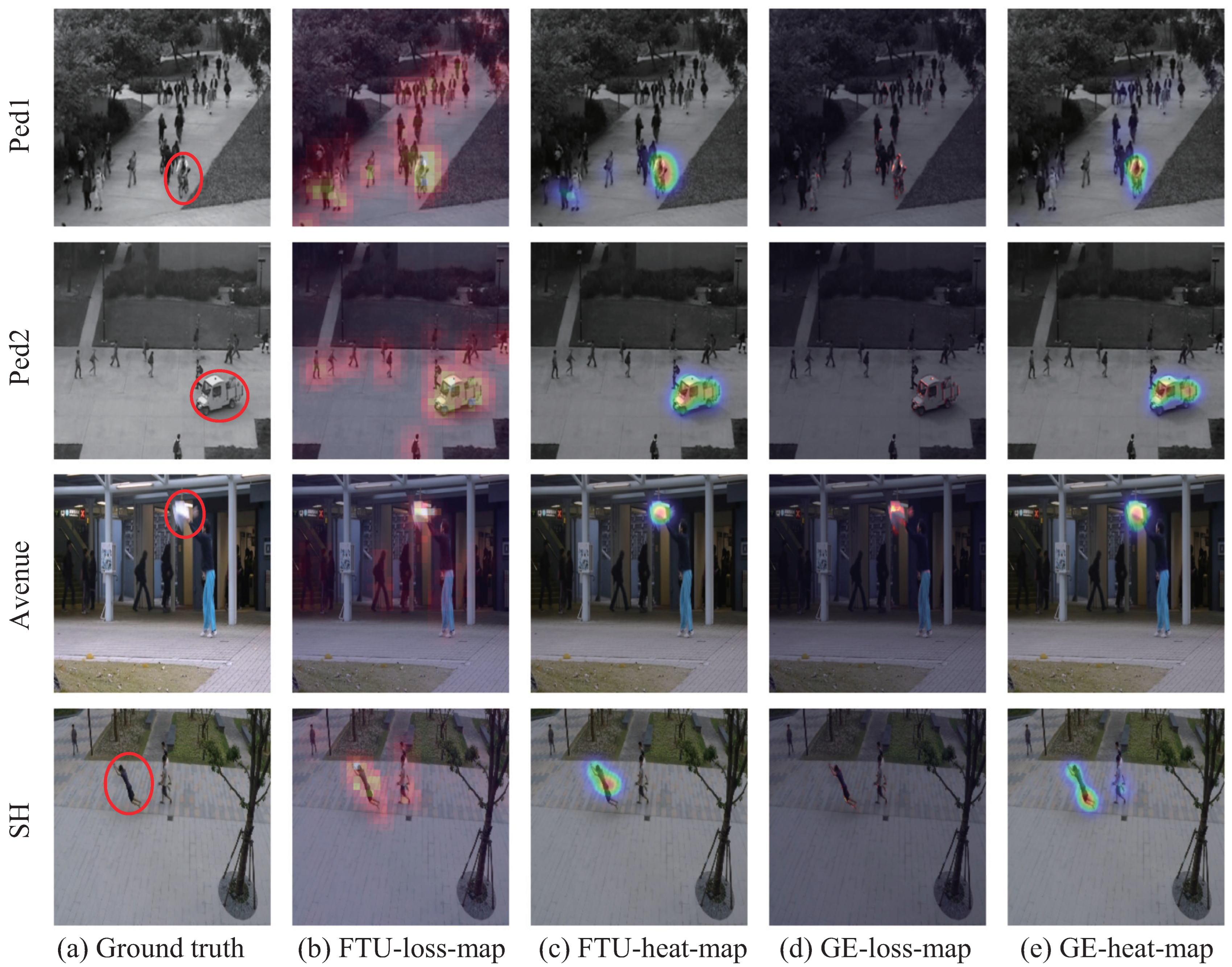
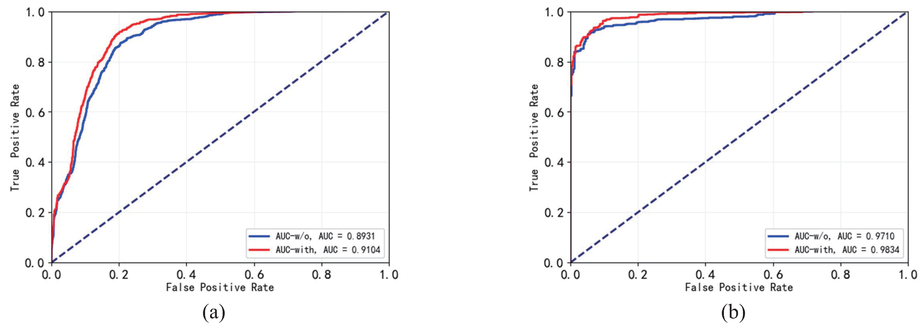
4.5.2. Impact of FTS Loss on the GE Detector
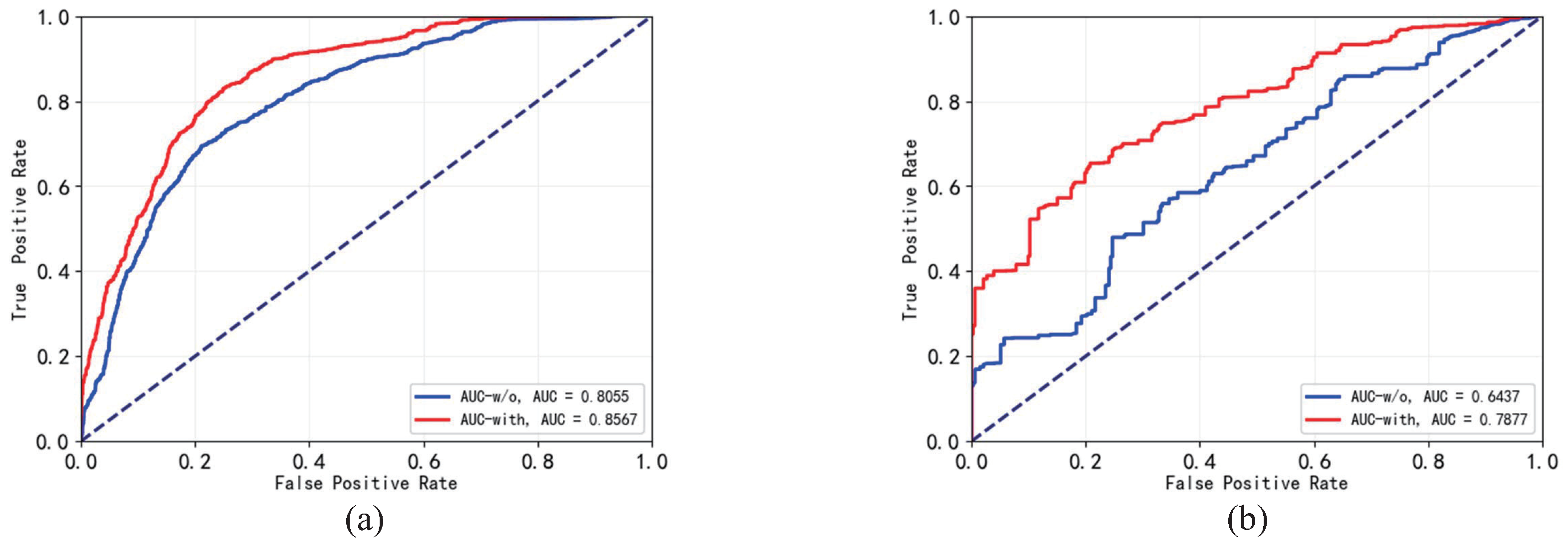
4.5.3. Impact of the FTS Loss on FTS Detector
4.5.4. Detection Speed Analysis
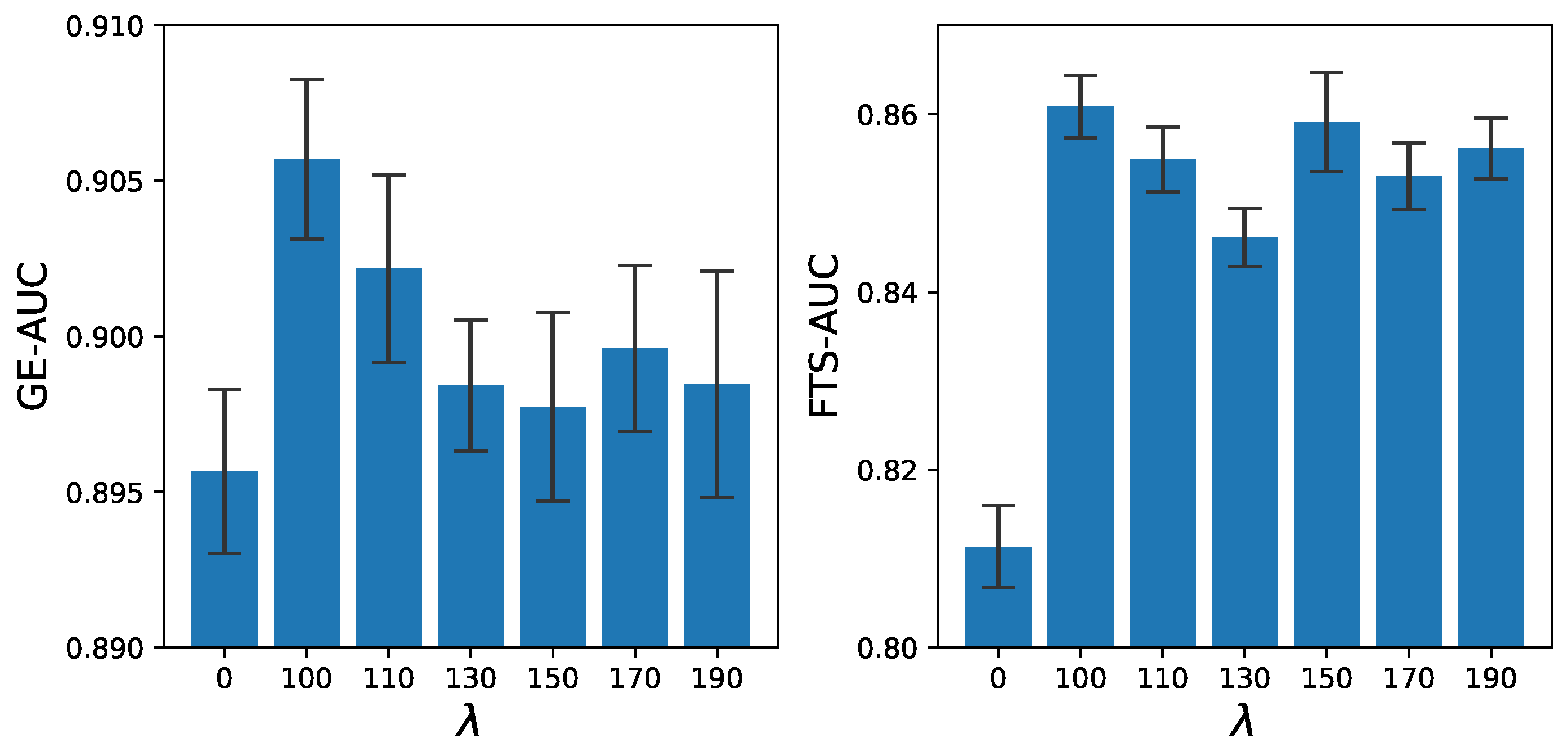
4.5.5. Impact of Weight
4.5.6. Generality
4.6. Limitation
5. Conclusions
Author Contributions
Funding
Institutional Review Board Statement
Informed Consent Statement
Data Availability Statement
Conflicts of Interest
References
- Xiao, T.; Zhang, C.; Zha, H. Learning to detect anomalies in surveillance video. IEEE Signal Process. Lett. 2015, 22, 1477–1481. [Google Scholar] [CrossRef]
- Prasad, N.R.; Almanza-Garcia, S.; Lu, T.T. Anomaly detection. Comput. Mater. Contin. 2009, 14, 1–22. [Google Scholar] [CrossRef]
- Kim, I.; Jeon, Y.; Kang, J.W.; Gwak, J. RAG-PaDiM: Residual Attention Guided PaDiM for Defects Segmentation in Railway Tracks. J. Electr. Eng. Technol. 2022. [Google Scholar] [CrossRef]
- Kang, J.; Kim, C.S.; Kang, J.W.; Gwak, J. Recurrent Autoencoder Ensembles for Brake Operating Unit Anomaly Detection on Metro Vehicles. Comput. Mater. Contin. 2022, 73, 1–4. [Google Scholar] [CrossRef]
- Kang, J.; Kim, C.S.; Kang, J.W.; Gwak, J. Anomaly detection of the brake operating unit on metro vehicles using a one-class lstm autoencoder. Appl. Sci. 2021, 11, 9290. [Google Scholar] [CrossRef]
- Zhang, T.; Aftab, W.; Mihaylova, L.; Langran-Wheeler, C.; Rigby, S.; Fletcher, D.; Maddock, S.; Bosworth, G. Recent Advances in Video Analytics for Rail Network Surveillance for Security, Trespass and Suicide Prevention—A Survey. Sensors 2022, 22, 4324. [Google Scholar] [CrossRef]
- Khan, S.W.; Hafeez, Q.; Khalid, M.I.; Alroobaea, R.; Hussain, S.; Iqbal, J.; Almotiri, J.; Ullah, S.S. Anomaly Detection in Traffic Surveillance Videos Using Deep Learning. Sensors 2022, 22, 6563. [Google Scholar] [CrossRef]
- Liu, W.; Luo, W.; Lian, D.; Gao, S. Future Frame Prediction for Anomaly Detection—A New Baseline. In Proceedings of the 2018 IEEE/CVF Conference on Computer Vision and Pattern Recognition, Salt Lake City, UT, USA, 18–22 June 2018; pp. 6536–6545. [Google Scholar] [CrossRef]
- Ullah, W.; Ullah, A.; Hussain, T.; Khan, Z.A.; Baik, S.W. An efficient anomaly recognition framework using an attention residual lstm in surveillance videos. Sensors 2021, 21, 2811. [Google Scholar] [CrossRef]
- Dubey, S.; Boragule, A.; Gwak, J.; Jeon, M. Anomalous event recognition in videos based on joint learning of motion and appearance with multiple ranking measures. Appl. Sci. 2021, 11, 1344. [Google Scholar] [CrossRef]
- Ionescu, R.T.; Smeureanu, S.; Alexe, B.; Popescu, M. Unmasking the Abnormal Events in Video. In Proceedings of the 2017 IEEE International Conference on Computer Vision (ICCV), Venice, Italy, 22–29 October 2017; pp. 2914–2922. [Google Scholar] [CrossRef]
- Oza, P.; Patel, V.M. One-Class Convolutional Neural Network. IEEE Signal Process. Lett. 2019, 26, 277–281. [Google Scholar] [CrossRef]
- Weixiang, J.; Gong, L. One-class neural network for video anomaly detection and localization. Electron. Meas. Instrum. 2021, 35, 60–65. [Google Scholar]
- Wu, P.; Liu, J.; Shen, F. A Deep One-Class Neural Network for Anomalous Event Detection in Complex Scenes. IEEE Trans. Neural Netw. Learn. Syst. 2019, 31, 2609–2622. [Google Scholar] [CrossRef] [PubMed]
- Abati, D.; Porrello, A.; Calderara, S.; Cucchiara, R. Latent space autoregression for novelty detection. In Proceedings of the IEEE Computer Society Conference on Computer Vision and Pattern Recognition, Long Beach, CA, USA, 16–17 June 2019; IEEE Computer Society: Washington, DC, USA, 2019; Volume 2019, pp. 481–490. [Google Scholar] [CrossRef]
- Wang, T.; Xu, X.; Shen, F.; Yang, Y. A Cognitive Memory-Augmented Network for Visual Anomaly Detection. IEEE/CAA J. Autom. Sin. 2021, 8, 1296–1307. [Google Scholar] [CrossRef]
- Sabokrou, M.; Pourreza, M.; Fayyaz, M.; Entezari, R.; Fathy, M.; Gall, J.; Adeli, E. AVID: Adversarial Visual Irregularity Detection. In Computer Vision—ACCV 2018, Proceedings of the 14th Asian Conference on Computer Vision, Perth, Australia, 2–6 December 2018; Lecture Notes in Computer Science (Including Subseries Lecture Notes in Artificial Intelligence and Lecture Notes in Bioinformatics); Springer: Cham, Switzerland, 2018; Volume 11366 LNCS, pp. 488–505. [Google Scholar] [CrossRef]
- Song, H.; Sun, C.; Wu, X.; Chen, M.; Jia, Y. Learning Normal Patterns via Adversarial Attention-Based Autoencoder for Abnormal Event Detection in Videos. IEEE Trans. Multimed. 2020, 22, 2138–2148. [Google Scholar] [CrossRef]
- Luo, W.; Liu, W.; Lian, D.; Tang, J.; Duan, L.; Peng, X.; Gao, S. Video Anomaly Detection with Sparse Coding Inspired Deep Neural Networks. IEEE Trans. Pattern Anal. Mach. Intell. 2021, 43, 1070–1084. [Google Scholar] [CrossRef]
- Tang, Y.; Zhao, L.; Zhang, S.; Gong, C.; Li, G.; Yang, J. Integrating prediction and reconstruction for anomaly detection. Pattern Recognit. Lett. 2020, 129, 123–130. [Google Scholar] [CrossRef]
- Lee, S.; Kim, H.G.; Ro, Y.M. STAN: Spatio-Temporal Adversarial Networks for Abnormal Event Detection. In Proceedings of the 2018 IEEE International Conference on Acoustics, Speech and Signal Processing (ICASSP), Calgary, AB, Canada, 15–20 April 2018; pp. 1323–1327. [Google Scholar] [CrossRef] [Green Version]
- Ji, X.; Li, B.; Zhu, Y. TAM-Net: Temporal Enhanced Appearance-to-Motion Generative Network for Video Anomaly Detection. In Proceedings of the 2020 International Joint Conference on Neural Networks (IJCNN), Glasgow, UK, 19–24 July 2020; pp. 1–8. [Google Scholar] [CrossRef]
- Wang, Z.; Zhang, Y.; Wang, G.; Xie, P. Main-Auxiliary Aggregation Strategy for Video Anomaly Detection. IEEE Signal Process. Lett. 2021, 28, 1794–1798. [Google Scholar] [CrossRef]
- Chong, Y.S.; Tay, Y.H. Abnormal Event Detection in Videos Using Spatiotemporal Autoencoder. In Advances in Neural Networks—ISNN 2017; Lecture Notes in Computer Science; Springer: Cham, Switzerland, 2017; Volume 10262, pp. 189–196. [Google Scholar] [CrossRef]
- Luo, W.; Liu, W.; Gao, S. Remembering history with convolutional LSTM for anomaly detection. In Proceedings of the 2017 IEEE International Conference on Multimedia and Expo (ICME), Hong Kong, China, 10–14 July 2017; pp. 439–444. [Google Scholar] [CrossRef]
- Hasan, M.; Choi, J.; Neumann, J.; Roy-Chowdhury, A.K.; Davis, L.S. Learning Temporal Regularity in Video Sequences. In Proceedings of the 2016 IEEE Conference on Computer Vision and Pattern Recognition (CVPR), Seattle, WA, USA, 27–30 June 2016; pp. 733–742. [Google Scholar] [CrossRef]
- Huang, C.; Wen, J.; Xu, Y.; Jiang, Q.; Yang, J.; Wang, Y.; Zhang, D. Self-Supervised Attentive Generative Adversarial Networks for Video Anomaly Detection. IEEE Trans. Neural Netw. Learn. Syst. 2022, 1–15. [Google Scholar] [CrossRef]
- Ionescu, R.T.; Smeureanu, S.; Popescu, M.; Alexe, B. Detecting Abnormal Events in Video Using Narrowed Normality Clusters. In Proceedings of the 2019 IEEE Winter Conference on Applications of Computer Vision (WACV), Waikoloa Village, HI, USA, 7–11 January 2019; pp. 1951–1960. [Google Scholar] [CrossRef]
- Hinami, R.; Mei, T.; Satoh, S. Joint Detection and Recounting of Abnormal Events by Learning Deep Generic Knowledge. In Proceedings of the 2017 IEEE International Conference on Computer Vision (ICCV), Venice, Italy, 22–29 October 2017; pp. 3639–3647. [Google Scholar] [CrossRef]
- Pruteanu-Malinici, I.; Carin, L. Infinite Hidden Markov Models for Unusual-Event Detection in Video. IEEE Trans. Image Process. 2008, 17, 811–822. [Google Scholar] [CrossRef]
- Xiang, T.; Gong, S. Incremental and adaptive abnormal behaviour detection. Comput. Vis. Image Underst. 2008, 111, 59–73. [Google Scholar] [CrossRef] [Green Version]
- Hu, X.; Huang, Y.; Gao, X.; Luo, L.; Duan, Q. Squirrel-cage local binary pattern and its application in video anomaly detection. IEEE Trans. Inf. Forensics Secur. 2019, 14, 1007–1022. [Google Scholar] [CrossRef]
- Gnouma, M.; Ejbali, R.; Zaied, M. Video Anomaly Detection and Localization in Crowded Scenes. Adv. Intell. Syst. Comput. 2020, 951, 87–96. [Google Scholar] [CrossRef]
- Lu, C.; Shi, J.; Jia, J. Abnormal Event Detection at 150 FPS in MATLAB. In Proceedings of the 2013 IEEE International Conference on Computer Vision, Sydney, NSW, Australia, 1–8 December 2013; pp. 2720–2727. [Google Scholar] [CrossRef]
- Cong, Y.; Yuan, J.; Liu, J. Sparse reconstruction cost for abnormal event detection. In Proceedings of the IEEE Computer Society Conference on Computer Vision and Pattern Recognition, Colorado Springs, CO, USA, 20–25 June 2011; pp. 3449–3456. [Google Scholar] [CrossRef]
- Chu, W.; Xue, H.; Yao, C.; Cai, D. Sparse Coding Guided Spatiotemporal Feature Learning for Abnormal Event Detection in Large Videos. IEEE Trans. Multimed. 2019, 21, 246–255. [Google Scholar] [CrossRef]
- Fan, Y.; Wen, G.; Li, D.; Qiu, S.; Levine, M.D.; Xiao, F. Video anomaly detection and localization via Gaussian Mixture Fully Convolutional Variational Autoencoder. Comput. Vis. Image Underst. 2020, 195, 102920. [Google Scholar] [CrossRef]
- Sabokrou, M.; Khalooei, M.; Fathy, M.; Adeli, E. Adversarially Learned One-Class Classifier for Novelty Detection. In Proceedings of the 2018 IEEE/CVF Conference on Computer Vision and Pattern Recognition, Salt Lake City, UT, USA, 18–22 June 2018; pp. 3379–3388. [Google Scholar] [CrossRef]
- Ravanbakhsh, M.; Nabi, M.; Sangineto, E.; Marcenaro, L.; Regazzoni, C.; Sebe, N. Abnormal event detection in videos using generative adversarial nets. In Proceedings of the 2017 IEEE International Conference on Image Processing (ICIP), Beijing, China, 17–20 September 2017; pp. 1577–1581. [Google Scholar] [CrossRef]
- Gong, D.; Liu, L.; Le, V.; Saha, B.; Mansour, M.R.; Venkatesh, S.; Van Den Hengel, A. Memorizing Normality to Detect Anomaly: Memory-Augmented Deep Autoencoder for Unsupervised Anomaly Detection. In Proceedings of the 2019 IEEE/CVF International Conference on Computer Vision (ICCV), Seoul, Republic of Korea, 27 October–2 November 2019; Volume 2019, pp. 1705–1714. [Google Scholar] [CrossRef]
- Zhou, J.T.; Zhang, L.; Fang, Z.; Du, J.; Peng, X.; Xiao, Y. Attention-Driven Loss for Anomaly Detection in Video Surveillance. IEEE Trans. Circuits Syst. Video Technol. 2020, 30, 4639–4647. [Google Scholar] [CrossRef]
- Medel, J.R.; Savakis, A. Anomaly Detection in Video Using Predictive Convolutional Long Short-Term Memory Networks. arXiv 2016, arXiv:1612.00390. [Google Scholar]
- Lu, Y.; Kumar, K.M.; Nabavi, S.S.; Wang, Y. Future Frame Prediction Using Convolutional VRNN for Anomaly Detection. In Proceedings of the 2019 16th IEEE International Conference on Advanced Video and Signal Based Surveillance (AVSS), Taipei, Taiwan, 18–21 September 2019; pp. 1–8. [Google Scholar] [CrossRef]
- Nair, V.; Hinton, G.E. Rectified Linear Units Improve Restricted Boltzmann Machines. In Proceedings of the 27th International Conference on International Conference on Machine Learning (ICML’10), Madison, WI, USA, 21–24 June 2010; pp. 807–814. [Google Scholar]
- Wang, Z.; Yang, Z.; Zhang, Y.J. A promotion method for generation error-based video anomaly detection. Pattern Recognit. Lett. 2020, 140, 88–94. [Google Scholar] [CrossRef]
- Mahadevan, V.; Li, W.; Bhalodia, V.; Vasconcelos, N. Anomaly detection in crowded scenes. In Proceedings of the 2010 IEEE Computer Society Conference on Computer Vision and Pattern Recognition, San Francisco, CA, USA, 13–18 June 2010; pp. 1975–1981. [Google Scholar] [CrossRef]
- Kingma, D.P.; Ba, J. Adam: A Method for Stochastic Optimization. arXiv 2014, arXiv:1412.6980. [Google Scholar]
- Wang, Z.; Yang, Z.; Zhang, Y.; Su, N.; Wang, G. Image and Graphics. In Ts-Unet: A Temporal Smoothed Unet for Video Anomaly Detection, Proceedings of the 11th International Conference on Image and Graphics, Shanghai, China, 13–15 September 2017; Springer: Berlin/Heidelberg, Germany, 2017; Volume 10666, pp. 447–461. [Google Scholar] [CrossRef]


| FTS Loss | Ped1 | Ped2 | Avenue | SH | |
|---|---|---|---|---|---|
| GE saliency of | w/o | 1.930 | 3.657 | 2.645 | 1.184 |
| Anomalous frames | with | 2.205 | 3.985 | 2.656 | 1.366 |
| ROC/AUC | w/o | 82.73 | 97.10 | 89.31 | 71.20 |
| with | 83.51 | 98.34 | 91.04 | 72.92 |
| FTS Loss | Ped1 | Ped2 | Avenue | SH | |
|---|---|---|---|---|---|
| FTS saliency of | w/o | 0.086 | 0.055 | 0.342 | 0.342 |
| Anomalous frames | with | 0.162 | 0.122 | 0.639 | 0.374 |
| ROC/AUC | w/o | 64.02 | 64.37 | 80.55 | 67.22 |
| with | 70.22 | 78.77 | 85.67 | 68.71 |
| ROC/AUC | Speed | ||||
|---|---|---|---|---|---|
| Ped1 | Ped2 | Avenue | SH | ||
| FTS Detector | 70.22 | 78.77 | 85.67 | 68.71 | 186 FPS |
| GE Detector | 83.51 | 98.34 | 91.04 | 72.92 | 50 FPS |
| Cascade | 83.51 | 98.34 | 91.14 | 72.92 | 117 FPS |
| FTS Loss | Ped2 | Avenue | Average | |
|---|---|---|---|---|
| Saliency of Anomalous frames | w/o | 0.9278 | 1.086 | 1.0007 |
| with | 1.104 | 1.192 | 1.148 | |
| ROC/AUC | w/o | 76.51 | 79.18 | 77.85 |
| with | 82.25 | 81.62 | 81.94 |
Disclaimer/Publisher’s Note: The statements, opinions and data contained in all publications are solely those of the individual author(s) and contributor(s) and not of MDPI and/or the editor(s). MDPI and/or the editor(s) disclaim responsibility for any injury to people or property resulting from any ideas, methods, instructions or products referred to in the content. |
© 2023 by the authors. Licensee MDPI, Basel, Switzerland. This article is an open access article distributed under the terms and conditions of the Creative Commons Attribution (CC BY) license (https://creativecommons.org/licenses/by/4.0/).
Share and Cite
Sun, L.; Wang, Z.; Zhang, Y.; Wang, G. A Feature-Trajectory-Smoothed High-Speed Model for Video Anomaly Detection. Sensors 2023, 23, 1612. https://doi.org/10.3390/s23031612
Sun L, Wang Z, Zhang Y, Wang G. A Feature-Trajectory-Smoothed High-Speed Model for Video Anomaly Detection. Sensors. 2023; 23(3):1612. https://doi.org/10.3390/s23031612
Chicago/Turabian StyleSun, Li, Zhiguo Wang, Yujin Zhang, and Guijin Wang. 2023. "A Feature-Trajectory-Smoothed High-Speed Model for Video Anomaly Detection" Sensors 23, no. 3: 1612. https://doi.org/10.3390/s23031612