

Circulant Singular Spectrum Analysis and Discrete Wavelet Transform for Automated Removal of EOG Artifacts from EEG Signals

Abstract
:1. Introduction
1.1. Motivation
1.2. Related Work
2. Materials and Methods
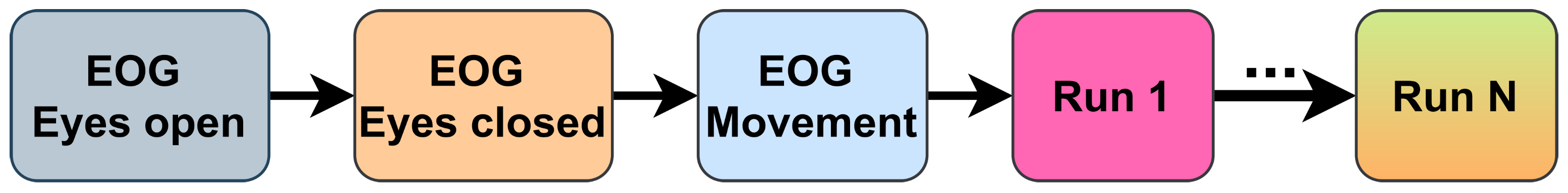
2.1. Materials
Signal Acquisition
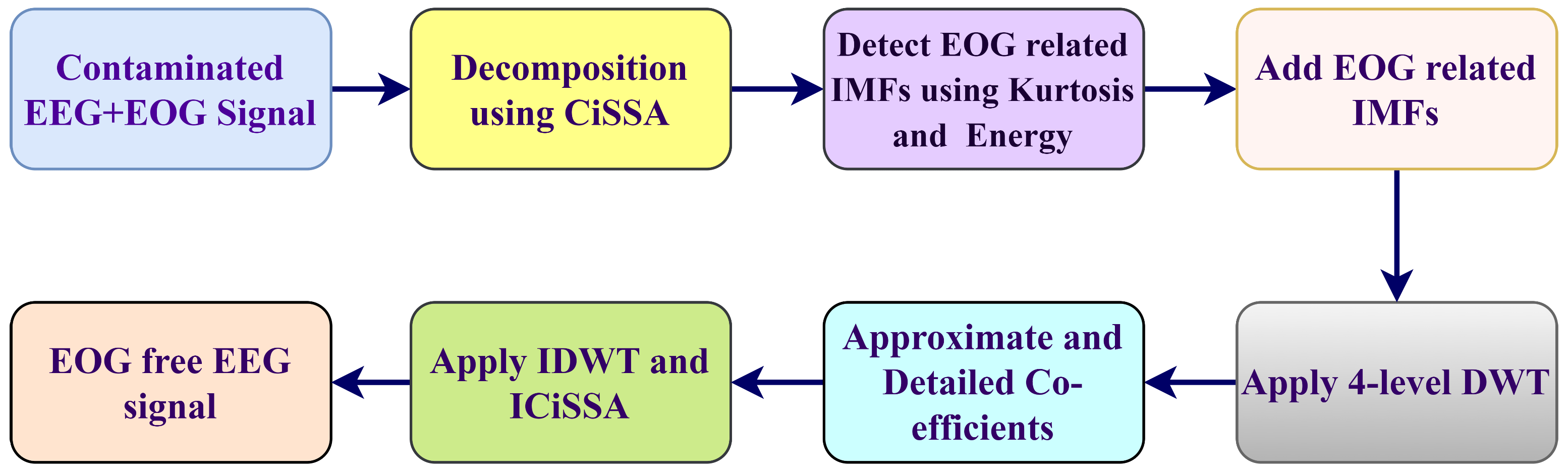
2.2. Methods
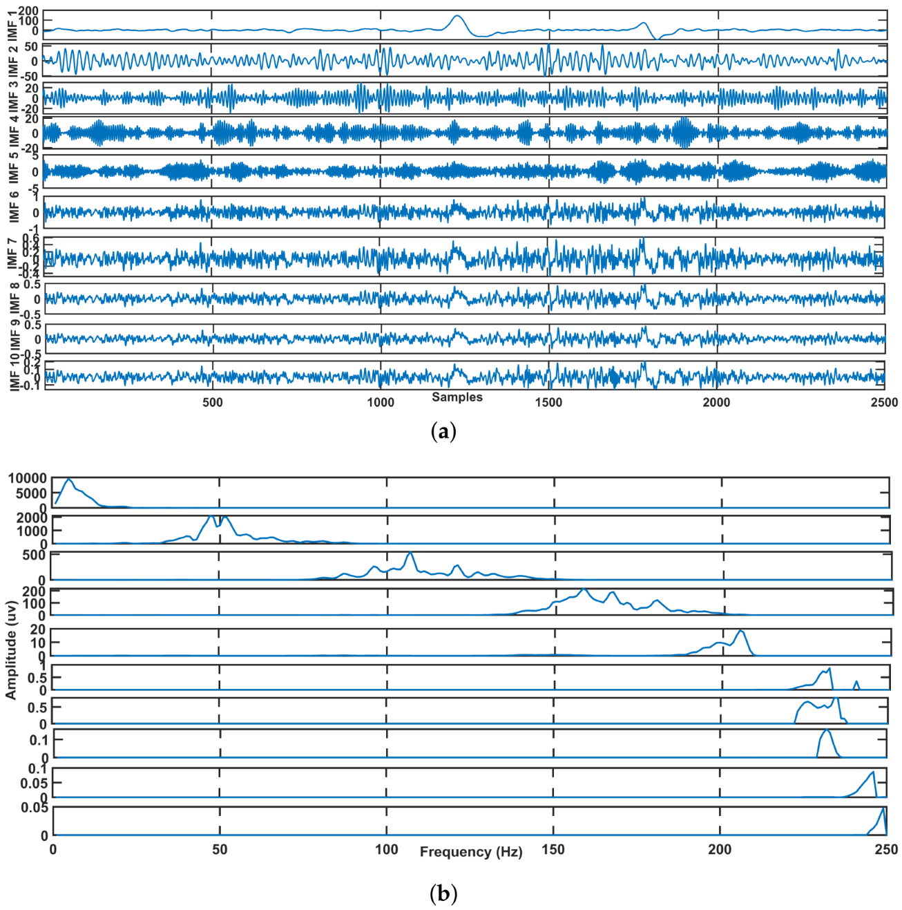
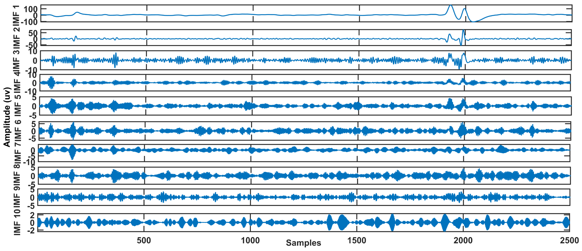
2.3. Decomposition of EEG Signals with CiSSA
- Step-1:
- Embedding In this step to construct a trajectory matrix A, , from the original time series as described in the following:where specifies the vector with origin at time.
- Step-2:
- Decomposition Construct the circulant matrix , which has the following components:calculate the eigenvalues of of as follows:Collaborate the kth eigenvalue and the corresponding eigenvector with frequency .
- Step-3:
- Grouping We obtain when we specify the analogy of power spectral density (PSD). Then, because their associated eigenvectors are complex, these are complex conjugate pairs, , where j* denotes the complex conjugate of j. To calculate related elements, we turn them into pairs of real eigenvectors. To make the fundamental matrixes, we’ll need to make two-element groups for with A1= 1 and if R is even. Then, using the frequency , compute the elementary matrix as the total of two elementary matrixes and , those are connected to the eigenvalues and and the frequency ,where is real part of , imaginary part is ,and denotes the conjugate transpose of j.
- Step-4:
- Reconstruction Each matrix is averaged diagonally to produce the newest time series of length t equal to the preceding one. It is equivalent to calculating the mean of the non-diagonal elements of , or hankelizing this matrix, which is denoted by the operator H (.). The Vautard-Ghil replacement, also known as the Toeplitz SSA, conducts orthogonal diagonalization from a different matrix under the premise that it is stationary and has a mean value of a non-zero average.
2.4. EOG Related IMFs Selection
2.4.1. Kurtosis
2.4.2. Energy
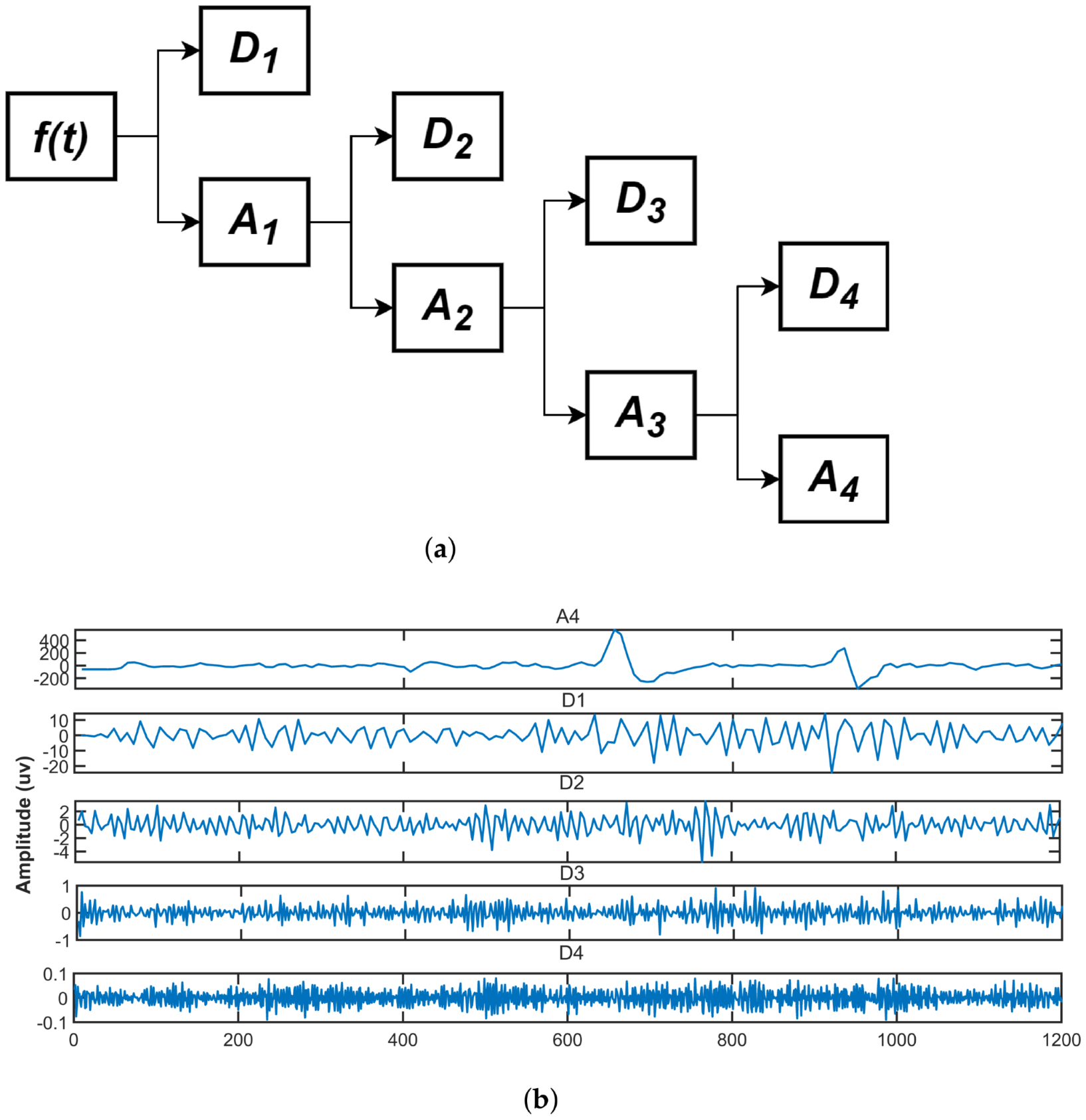
2.5. EOG Component Decomposition Using DWT
2.6. EEG Signal Reconstruction without EOG
Inverse DWT and CiSSA
3. Performance Metrics
3.1. RRMSE
3.2. CC
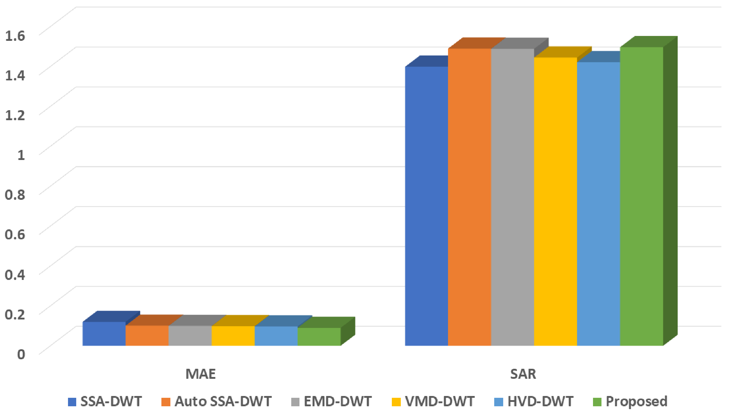
3.3. SAR
3.4. MAE
4. Results
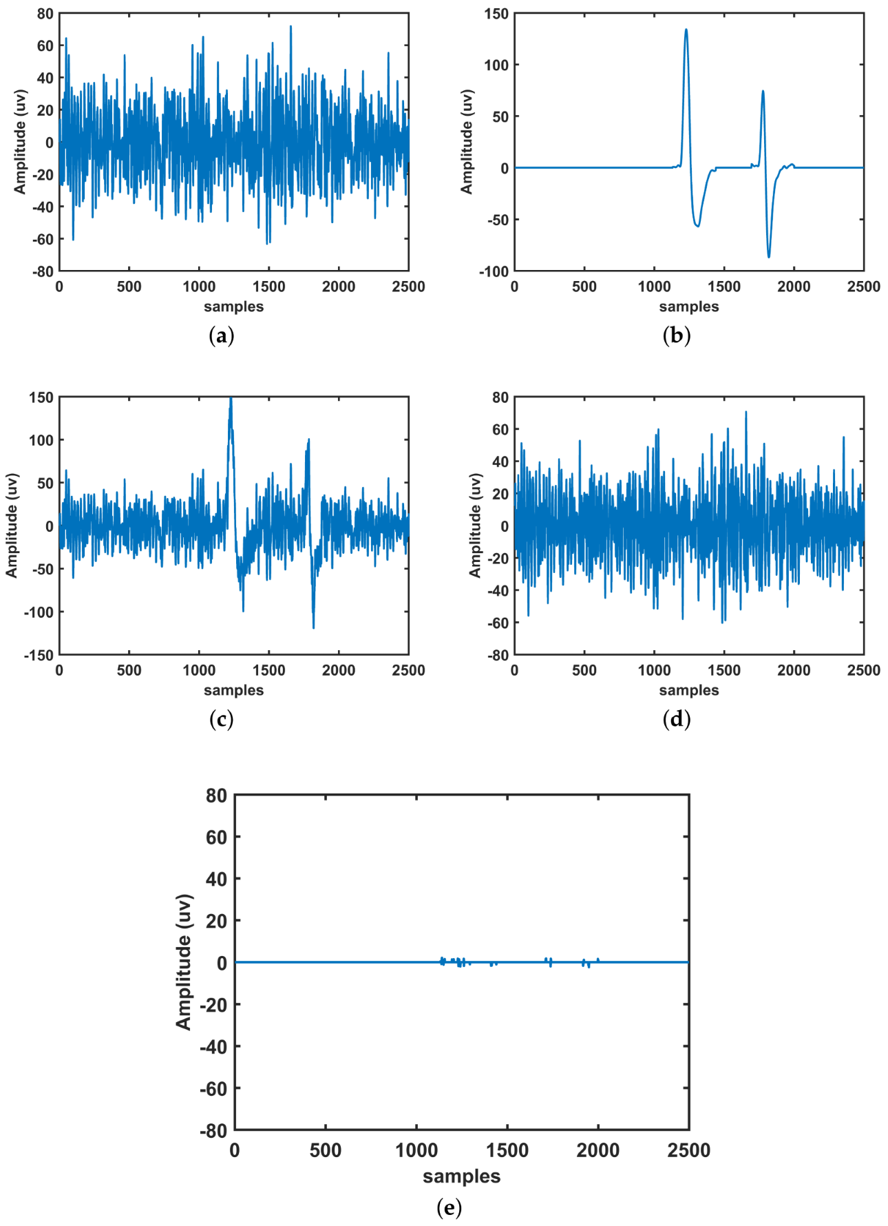
4.1. Synthetic EEG Signal Results
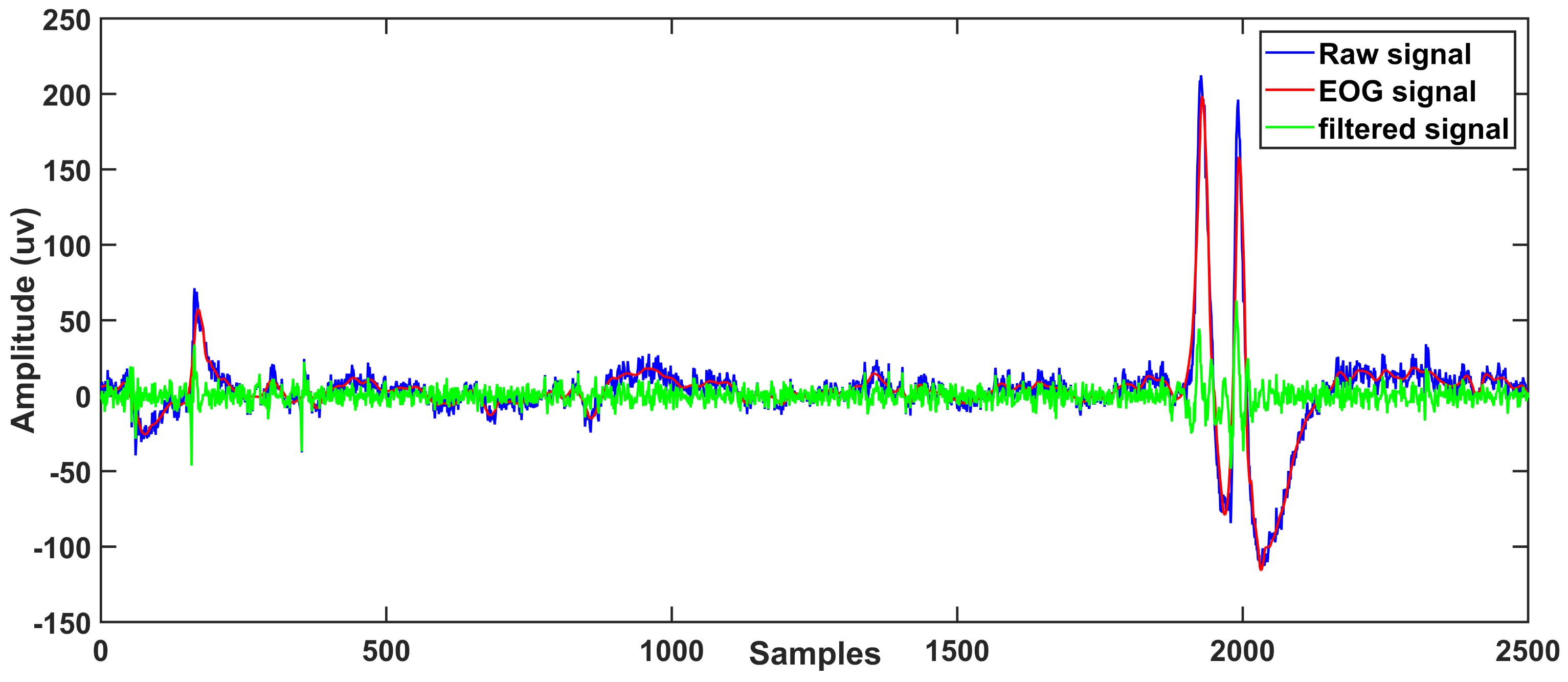
4.2. Real EEG Signal Results
5. Discussion
- The machine learning algorithms are not entirely explored in this research domain. Therefore, the scope of machine learning and deep learning approaches in ocular artifact removal from the EEG signal should be expanded.
- Hybrid approaches should be enhanced with some additional processing stages to eliminate all the types of artifacts present in the EEG signal, as hybrid yields promising results and is growing in this area of research.
- Advancements should be made to prior algorithms to develop a uniform criterion for the validation of EEG signals acquired in clinical studies.
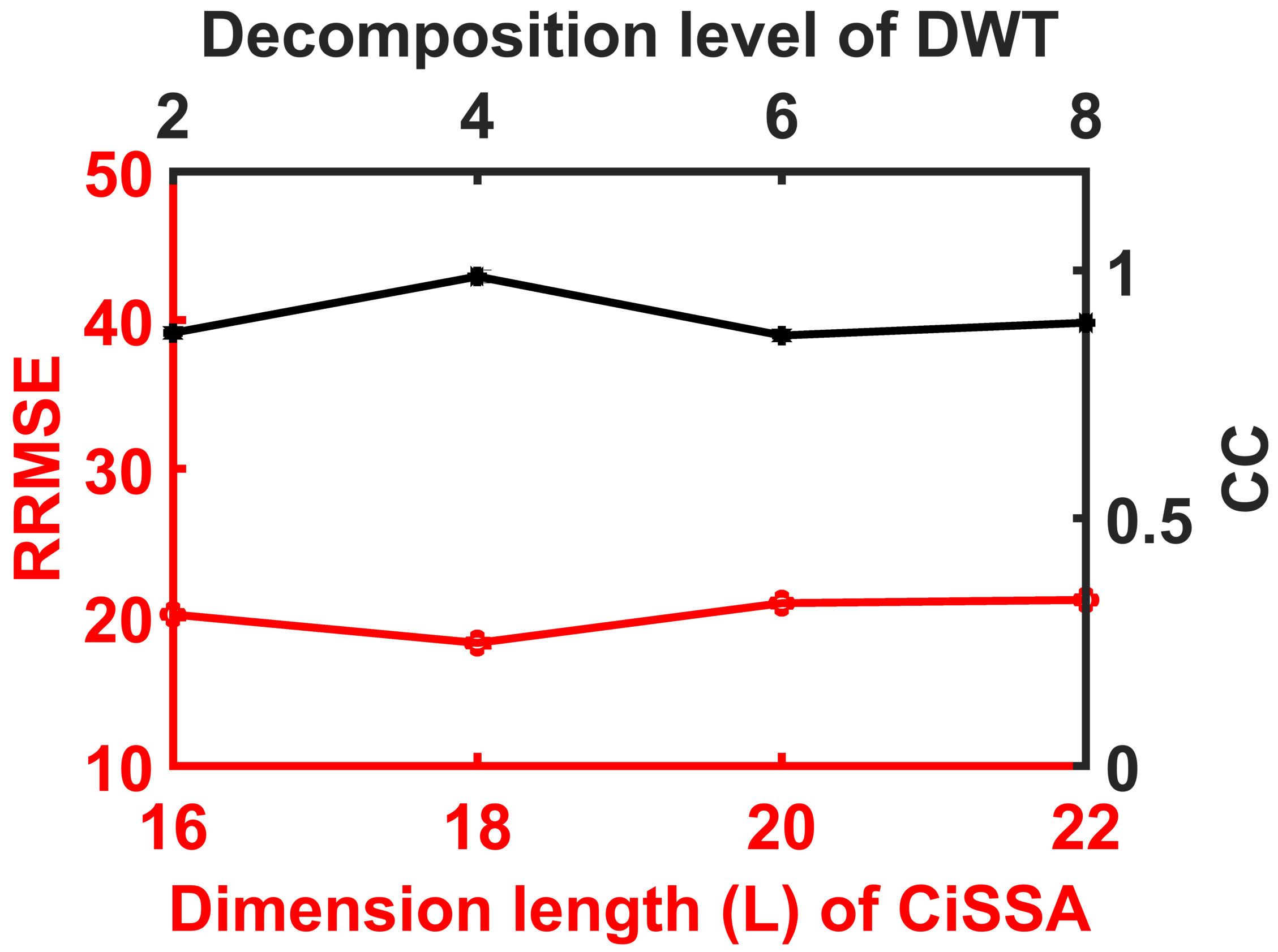
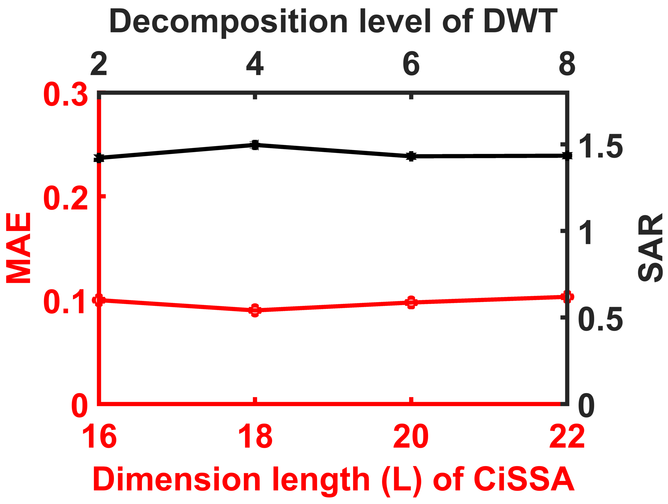
Experiment on Parameters Tuning
6. Conclusions
Author Contributions
Funding
Institutional Review Board Statement
Informed Consent Statement
Data Availability Statement
Conflicts of Interest
References
- Robinson, N.; Vinod, A.P.; Ang, K.K.; Tee, K.P.; Guan, C.T. EEG-based classification of fast and slow hand movements using wavelet-CSP algorithm. IEEE Trans. Biomed. Eng. 2013, 60, 2123–2132. [Google Scholar] [CrossRef] [PubMed]
- Guo, Z.; Pan, Y.; Zhao, G.; Cao, S.; Zhang, J. Detection of driver vigilance level using EEG signals and driving contexts. IEEE Trans. Reliab. 2017, 67, 370–380. [Google Scholar] [CrossRef]
- Noachtar, S.; Rémi, J. The role of EEG in epilepsy: A critical review. Epilepsy Behav. 2009, 15, 22–33. [Google Scholar] [CrossRef] [PubMed]
- Ofner, P.; Schwarz, A.; Pereira, J.; Wyss, D.; Wildburger, R.; Müller-Putz, G.R. Attempted arm and hand movements can be decoded from low-frequency EEG from persons with spinal cord injury. Sci. Rep. 2019, 9, 7134. [Google Scholar] [CrossRef] [PubMed] [Green Version]
- Sharma, L.D.; Saraswat, R.K.; Sunkaria, R.K. Cognitive performance detection using entropy-based features and lead-specific approach. Signal Image Video Process. 2021, 15, 1821–1828. [Google Scholar] [CrossRef]
- Veluvolu, K.C.; Wang, Y.; Kavuri, S.S. Adaptive estimation of EEG-rhythms for optimal band identification in BCI. J. Neurosci. Methods 2012, 203, 163–172. [Google Scholar] [CrossRef]
- Wang, Y.; Veluvolu, K.C.; Lee, M. Time-frequency analysis of band-limited EEG with BMFLC and Kalman filter for BCI applications. J. Neuroeng. Rehabil. 2013, 10, 109. [Google Scholar] [CrossRef] [Green Version]
- Halder, S.; Bensch, M.; Mellinger, J.; Bogdan, M.; Kübler, A.; Birbaumer, N.; Rosenstiel, W. Online artifact removal for brain–computer interfaces using support vector machines and blind source separation. Comput. Intell. Neurosci. 2007, 2007, 82069. [Google Scholar] [CrossRef] [Green Version]
- Hagemann, D.; Naumann, E. The effects of ocular artifacts on (lateralized) broadband power in the EEG. Clin. Neurophysiol. 2001, 112, 215–231. [Google Scholar] [CrossRef]
- Mannan, M.; Naeem, M.; Kamran, M.A.; Jeong, M.Y. Identification and removal of physiological artifacts from electroencephalogram signals: A review. IEEE Access 2018, 6, 30630–30652. [Google Scholar] [CrossRef]
- Patel, R.; Sengottuvel, S.; Janawadkar, M.; Gireesan, K.; Radhakrishnan, T.; Mariyappa, N. Ocular artifact suppression from EEG using ensemble empirical mode decomposition with principal component analysis. Comput. Electr. Eng. 2016, 54, 78–86. [Google Scholar] [CrossRef]
- Somers, B.; Francart, T.; Bertrand, A. A generic EEG artifact removal algorithm based on the multi-channel Wiener filter. J. Neural Eng. 2018, 15, 036007. [Google Scholar] [CrossRef]
- Noorbasha, S.K.; Sudha, G.F. Removal of EOG artifacts from single channel EEG—An efficient model combining overlap segmented ASSA and ANC. Biomed. Signal Process. Control 2020, 60, 101987. [Google Scholar] [CrossRef]
- Noorbasha, S.K.; Sudha, G.F. Removal of EOG artifacts and separation of different cerebral activity components from single channel EEG—An efficient approach combining SSA–ICA with wavelet thresholding for BCI applications. Biomed. Signal Process. Control 2021, 63, 102168. [Google Scholar] [CrossRef]
- Islam, M.K.; Rastegarnia, A.; Yang, Z. Methods for artifact detection and removal from scalp EEG: A review. Neurophysiol. Clin. Neurophysiol. 2016, 46, 287–305. [Google Scholar] [CrossRef]
- Vigário, R.; Sarela, J.; Jousmiki, V.; Hamalainen, M.; Oja, E. Independent component approach to the analysis of EEG and MEG recordings. IEEE Trans. Biomed. Eng. 2000, 47, 589–593. [Google Scholar] [CrossRef] [Green Version]
- De Clercq, W.; Vergult, A.; Vanrumste, B.; Van Paesschen, W.; Van Huffel, S. Canonical correlation analysis applied to remove muscle artifacts from the electroencephalogram. IEEE Trans. Biomed. Eng. 2006, 53, 2583–2587. [Google Scholar] [CrossRef]
- Delorme, A.; Sejnowski, T.; Makeig, S. Enhanced detection of artifacts in EEG data using higher-order statistics and independent component analysis. Neuroimage 2007, 34, 1443–1449. [Google Scholar] [CrossRef] [Green Version]
- Gao, J.; Zheng, C.; Wang, P. Online removal of muscle artifact from electroencephalogram signals based on canonical correlation analysis. Clin. EEG Neurosci. 2010, 41, 53–59. [Google Scholar] [CrossRef]
- Wang, G.; Teng, C.; Li, K.; Zhang, Z.; Yan, X. The removal of EOG artifacts from EEG signals using independent component analysis and multivariate empirical mode decomposition. IEEE J. Biomed. Health Inform. 2015, 20, 1301–1308. [Google Scholar] [CrossRef]
- Issa, M.F.; Juhasz, Z. Improved EOG artifact removal using wavelet enhanced independent component analysis. Brain Sci. 2019, 9, 355. [Google Scholar] [CrossRef] [PubMed] [Green Version]
- Castellanos, N.P.; Makarov, V.A. Recovering EEG brain signals: Artifact suppression with wavelet enhanced independent component analysis. J. Neurosci. Methods 2006, 158, 300–312. [Google Scholar] [CrossRef] [PubMed]
- Chang, C.Y.; Hsu, S.H.; Pion-Tonachini, L.; Jung, T.P. Evaluation of artifact subspace reconstruction for automatic artifact components removal in multi-channel EEG recordings. IEEE Trans. Biomed. Eng. 2019, 67, 1114–1121. [Google Scholar] [CrossRef] [PubMed]
- Yadavalli, M.K.; Pamula, V.K. An Efficient Framework to Automatic Extract EOG Artifacts from Single Channel EEG Recordings. In Proceedings of the 2022 IEEE International Conference on Signal Processing and Communications (SPCOM), Bangalore, India, 11–15 July 2022; IEEE: Piscataway, NJ, USA, 2022. [Google Scholar]
- Mshali, H.; Lemlouma, T.; Moloney, M.; Magoni, D. A survey on health monitoring systems for health smart homes. Int. J. Ind. Ergon. 2018, 66, 26–56. [Google Scholar] [CrossRef] [Green Version]
- Koley, B.; Dey, D. An ensemble system for automatic sleep stage classification using single channel EEG signal. Comput. Biol. Med. 2012, 42, 1186–1195. [Google Scholar] [CrossRef]
- Ogino, M.; Kanoga, S.; Muto, M.; Mitsukura, Y. Analysis of prefrontal single-channel EEG data for portable auditory ERP-based brain–computer interfaces. Front. Hum. Neurosci. 2019, 13, 250. [Google Scholar] [CrossRef]
- Quiroga, R.Q.; Atienza, M.; Cantero, J.L.; Jongsma, M.L.A. What can we learn from single-trial event-related potentials? Chaos Complex. Lett. 2007, 2, 345–363. [Google Scholar]
- Quiroga, R.Q.; Garcia, H. Single-trial event-related potentials with wavelet denoising. Clin. Neurophysiol. 2003, 114, 376–390. [Google Scholar] [CrossRef]
- Fatourechi, M.; Mason, S.G.; Birch, G.E.; Ward, R.K. A wavelet-based approach for the extraction of event related potentials from EEG. In Proceedings of the 2004 IEEE International Conference on Acoustics, Speech, and Signal Processing, Montreal, QC, Canada, 17–21 May 2004; IEEE: Piscataway, NJ, USA, 2004; Volume 2. [Google Scholar]
- Grosselin, F.; Navarro-Sune, X.; Vozzi, A.; Pandremmenou, K.; De Vico Fallani, F.; Attal, Y.; Chavez, M. Quality assessment of single-channel EEG for wearable devices. Sensors 2019, 19, 601. [Google Scholar] [CrossRef] [Green Version]
- Rogers, J.M.; Johnstone, S.J.; Aminov, A.; Donnelly, J.; Wilson, P.H. Test-retest reliability of a single-channel, wireless EEG system. Int. J. Psychophysiol. 2016, 106, 87–96. [Google Scholar] [CrossRef] [Green Version]
- He, P.; Wilson, G.; Russell, C. Removal of ocular artifacts from electro-encephalogram by adaptive filtering. Med Biol. Eng. Comput. 2004, 42, 407–412. [Google Scholar] [CrossRef]
- Peng, H.; Hu, B.; Shi, Q.; Ratcliffe, M.; Zhao, Q.; Qi, Y.; Gao, G. Removal of ocular artifacts in EEG—An improved approach combining DWT and ANC for portable applications. IEEE J. Biomed. Health Inform. 2013, 17, 600–607. [Google Scholar] [CrossRef]
- Abd Rahman, F.; Othman, M.F. Real time eye blink artifacts removal in electroencephalogram using savitzky-golay referenced adaptive filtering. In Proceedings of the International Conference for Innovation in Biomedical Engineering and Life Sciences, Putrajaya, Malaysia, 6–8 December 2015; Springer: Singapore, 2015. [Google Scholar]
- Shahbakhti, M.; Beiramvand, M.; Nazari, M.; Broniec-Wójcik, A.; Augustyniak, P.; Rodrigues, A.S.; Wierzchon, M.; Marozas, V. VME-DWT: An efficient algorithm for detection and elimination of eye blink from short segments of single EEG channel. IEEE Trans. Neural Syst. Rehabil. Eng. 2021, 29, 408–417. [Google Scholar] [CrossRef]
- Wu, Q.; Zhang, W.; Wang, Y.; Zhang, W.; Liu, X. Research on removal algorithm of EOG artifacts in single-channel EEG signals based on CEEMDAN-BD. Comput. Methods Biomech. Biomed. Eng. 2021, 24, 1368–1379. [Google Scholar] [CrossRef]
- Liu, T.; Luo, Z.; Huang, J.; Yan, S. A comparative study of four kinds of adaptive decomposition algorithms and their applications. Sensors 2018, 18, 2120. [Google Scholar] [CrossRef] [Green Version]
- Liu, C.; Zhang, C. Remove Artifacts from a Single-Channel EEG Based on VMD and SOBI. Sensors 2022, 22, 6698. [Google Scholar] [CrossRef]
- Golyandina, N.; Nekrutkin, V.; Zhigljavsky, A.A. Analysis of Time Series Structure: SSA and Related Techniques; CRC Press: Boca Raton, FL, USA, 2001. [Google Scholar]
- Maddirala, A.K.; Veluvolu, K.C. SSA with CWT and k-Means for Eye-Blink Artifact Removal from Single-Channel EEG Signals. Sensors 2022, 22, 931. [Google Scholar] [CrossRef]
- Sanei, S.; Lee, T.K.M.; Abolghasemi, V. A new adaptive line enhancer based on singular spectrum analysis. IEEE Trans. Biomed. Eng. 2011, 59, 428–434. [Google Scholar] [CrossRef]
- Mukhopadhyay, S.K.; Krishnan, S. A singular spectrum analysis-based model-free electrocardiogram denoising technique. Comput. Methods Programs Biomed. 2020, 188, 105304. [Google Scholar] [CrossRef]
- Maddirala, A.K.; Shaik, R.A. Motion artifact removal from single channel electroencephalogram signals using singular spectrum analysis. Biomed. Signal Process. Control 2016, 30, 79–85. [Google Scholar] [CrossRef]
- Teixeira, A.R.; Tome, A.M.; Lang, E.W.; Gruber, P.; da Silva, A.M. On the use of clustering and local singular spectrum analysis to remove ocular artifacts from electroencephalograms. In Proceedings of the 2005 IEEE International Joint Conference on Neural Networks, Montreal, QC, Canada, 31 July–4 August 2005; IEEE: Piscataway, NJ, USA, 2005; Volume 4. [Google Scholar]
- Maddirala, A.K.; Shaik, R.A. Removal of EOG artifacts from single channel EEG signals using combined singular spectrum analysis and adaptive noise canceler. IEEE Sens. J. 2016, 16, 8279–8287. [Google Scholar] [CrossRef]
- Maddirala, A.K.; Shaik, R.A. Separation of sources from single-channel EEG signals using independent component analysis. IEEE Trans. Instrum. Meas. 2017, 67, 382–393. [Google Scholar] [CrossRef]
- Maddirala, A.K.; Veluvolu, K.C. Eye-blink artifact removal from single channel EEG with k-means and SSA. Sci. Rep. 2021, 11, 11043. [Google Scholar] [CrossRef] [PubMed]
- Bógalo, J.; Poncela, P.; Senra, E. Circulant singular spectrum analysis: A new automated procedure for signal extraction. Signal Process. 2021, 179, 107824. [Google Scholar] [CrossRef]
- Bógalo, J.; Poncela, P.; Senra, E. Automatic Signal Extraction for Stationary and Non-Stationary Time Series by Circulant SSA; University Library of Munich: Munich, Germany, 2017. [Google Scholar]
- Tangermann, M.; Müller, K.R.; Aertsen, A.; Birbaumer, N.; Braun, C.; Brunner, C.; Leeb, R.; Mehring, C.; Miller, K.J.; Mueller-Putz, G.; et al. Review of the BCI competition IV. Front. Neurosci. 2012, 6, 55. [Google Scholar]
- Yedukondalu, J.; Sharma, L.D. Cognitive load detection using circulant singular spectrum analysis and Binary Harris Hawks Optimization based feature selection. Biomed. Signal Process. Control 2023, 79, 104006. [Google Scholar] [CrossRef]
- Yedukondalu, J.; Sharma, L.D. Cognitive load detection using Binary salp swarm algorithm for feature selection. In Proceedings of the 2022 IEEE 6th Conference on Information and Communication Technology (CICT), Gwalior, India, 18–20 November 2022; pp. 1–5. [Google Scholar] [CrossRef]
- Hu, H.; Pu, Z.; Li, H.; Liu, Z.; Wang, P. Learning Optimal Time-Frequency-Spatial Features by the CiSSA-CSP Method for Motor Imagery EEG Classification. Sensors 2022, 22, 8526. [Google Scholar] [CrossRef]
- Klados, M.A.; Bamidis, P.D. A semi-simulated EEG/EOG dataset for the comparison of EOG artifact rejection techniques. Data Brief 2016, 8, 1004–1006. [Google Scholar] [CrossRef] [Green Version]
- Mijović, B.; De Vos, M.; Gligorijević, I.; Taelman, J.; Van Huffel, S. Source separation from single-channel recordings by combining empirical-mode decomposition and independent component analysis. IEEE Trans. Biomed. Eng. 2010, 57, 2188–2196. [Google Scholar] [CrossRef]
- Inuso, G.; La Foresta, F.; Mammone, N.; Morabito, F.C. Wavelet-ICA methodology for efficient artifact removal from Electroencephalographic recordings. In Proceedings of the 2007 International Joint Conference on Neural Networks, Orlando, FL, USA, 12–17 August 2007; IEEE: Piscataway, NJ, USA, 2007. [Google Scholar]
- Zhang, S.; McIntosh, J.; Shadli, S.M.; Neo, P.S.; Huang, Z.; McNaughton, N. Removing eye blink artefacts from EEG—A single-channel physiology-based method. J. Neurosci. Methods 2017, 291, 213–220. [Google Scholar] [CrossRef]
- Gajbhiye, P.; Tripathy, R.K.; Pachori, R.B. Elimination of ocular artifacts from single channel EEG signals using FBSE-EWT based rhythms. IEEE Sens. J. 2019, 20, 3687–3696. [Google Scholar] [CrossRef]
- Dragomiretskiy, K.; Zosso, D. Variational mode decomposition. IEEE Trans. Signal Process. 2013, 62, 531–544. [Google Scholar] [CrossRef]
- Feldman, M. Time-varying vibration decomposition and analysis based on the Hilbert transform. J. Sound Vib. 2006, 295, 518–530. [Google Scholar] [CrossRef]
- Sharma, L.D.; Bohat, V.K.; Habib, M.; Ala’M, A.Z.; Faris, H.; Aljarah, I. Evolutionary inspired approach for mental stress detection using EEG signal. Expert Syst. Appl. 2022, 197, 116634. [Google Scholar] [CrossRef]
- Sharma, L.D.; Chhabra, H.; Chauhan, U.; Saraswat, R.K.; Sunkaria, R.K. Mental arithmetic task load recognition using EEG signal and Bayesian optimized K-nearest neighbor. Int. J. Inf. Technol. 2021, 13, 2363–2369. [Google Scholar] [CrossRef]
- Sharma, L.D.; Bhattacharyya, A. A computerized approach for automatic human emotion recognition using sliding mode singular spectrum analysis. IEEE Sens. J. 2021, 21, 26931–26940. [Google Scholar] [CrossRef]
- Vempati, R.; Sharma, L.D. EOG Eye Blink Artifact Removal using Multivariate Variational Mode Decomposition and PCA. In Proceedings of the 2022 IEEE 6th Conference on Information and Communication Technology (CICT), Gwalior, India, 18–20 November 2022; pp. 1–5. [Google Scholar] [CrossRef]


| Artifact Mixing Constant (p) | RRMSE | CC |
|---|---|---|
| p = 0.5 | 29.8156 | 0.9686 |
| p = 1 | 18.2743 | 0.9883 |
| p = 1.25 | 15.1146 | 0.9892 |
| p = 1.5 | 12.1584 | 0.9935 |
| Subjects | Records | ||||||||
|---|---|---|---|---|---|---|---|---|---|
| R-1 | R-2 | R-3 | R-4 | R-5 | R-6 | R-7 | R-8 | Average | |
| Subject 1 | 0.0901 | 0.0855 | 0.0824 | 0.0908 | 0.0800 | 0.0787 | 0.0970 | 0.0852 | 0.0862 |
| Subject 2 | 0.1034 | 0.0917 | 0.0996 | 0.0899 | 0.0777 | 0.0889 | 0.0794 | 0.0901 | 0.0900 |
| Subject 3 | 0.0806 | 0.0881 | 0.0999 | 0.0834 | 0.0801 | 0.088 | 0.0911 | 0.0887 | 0.0874 |
| Subject 4 | 0.0855 | 0.0712 | 0.0767 | 0.0786 | 0.0842 | 0.0789 | 0.0799 | 0.0863 | 0.0801 |
| Subject 5 | 0.0933 | 0.0899 | 0.0779 | 0.1000 | 0.0810 | 0.0872 | 0.0909 | 0.0869 | 0.0883 |
| Subject 6 | 0.0900 | 0.0891 | 0.0893 | 0.0781 | 0.0910 | 0.0842 | 0.0999 | 0.0794 | 0.0876 |
| Subject 7 | 0.0934 | 0.0812 | 0.0895 | 0.0887 | 0.0745 | 0.0877 | 0.0774 | 0.0885 | 0.0851 |
| Subject 8 | 0.0843 | 0.0784 | 0.0796 | 0.0896 | 0.0892 | 0.0888 | 0.0909 | 0.0772 | 0.0847 |
| Subject 9 | 0.0981 | 0.0912 | 0.0886 | 0.0987 | 0.0871 | 0.0788 | 0.0804 | 0.0900 | 0.0891 |
| Subjects | Records | ||||||||
|---|---|---|---|---|---|---|---|---|---|
| R-1 | R-2 | R-3 | R-4 | R-5 | R-6 | R-7 | R-8 | Average | |
| Subject 1 | 1.399 | 1.497 | 1.410 | 1.320 | 1.278 | 1.271 | 1.355 | 1.389 | 1.362 |
| Subject 2 | 1.394 | 1.454 | 1.352 | 1.313 | 1.324 | 1.356 | 1.311 | 1.291 | 1.349 |
| Subject 3 | 1.237 | 1.401 | 1.131 | 1.401 | 1.410 | 1.322 | 1.404 | 1.314 | 1.328 |
| Subject 4 | 1.394 | 1.552 | 1.445 | 1.407 | 1.412 | 1.453 | 1.476 | 1.481 | 1.453 |
| Subject 5 | 1.121 | 1.259 | 1.261 | 1.211 | 1.228 | 1.265 | 1.110 | 1.121 | 1.197 |
| Subject 6 | 1.330 | 1.260 | 1.347 | 1.424 | 1.385 | 1.410 | 1.300 | 1.427 | 1.360 |
| Subject 7 | 1.402 | 1.120 | 1.220 | 1.400 | 1.444 | 1.268 | 1.405 | 1.200 | 1.307 |
| Subject 8 | 1.279 | 1.335 | 1.290 | 1.369 | 1.284 | 1.318 | 1.264 | 1.287 | 1.303 |
| Subject 9 | 1.333 | 1.399 | 1.305 | 1.461 | 1.290 | 1.375 | 1.463 | 1.412 | 1.380 |
| Authors | Methodology | p = 0.5 | p = 1 | p = 1.25 | p = 1.5 | ||||
|---|---|---|---|---|---|---|---|---|---|
| RRMSE | CC | RRMSE | CC | RRMSE | CC | RRMSE | CC | ||
| B. Mijovic et al. [56] | EEMD-ICA | 67.8152 | 0.8297 | 37.485 | 0.9358 | 31.212 | 0.9529 | 26.863 | 0.964 |
| Giuseppina Inuso et al. [57] | SSA-ICA | 61.1533 | 0.8522 | 32.585 | 0.9499 | 27.21 | 0.964 | 22.78 | 0.9746 |
| Zhang, S. et al. [58] | Infomax and FastICA | 42.4855 | 0.9159 | 20.168 | 0.9754 | 18.632 | 0.9794 | 16.283 | 0.9819 |
| Gajbhiye, P. et al. [59] | FBSE-EWT | 31.3118 | 0.9513 | 20.203 | 0.9801 | 17.067 | 0.9858 | 14.709 | 0.9895 |
| Proposed | CiSSA-DWT | 29.8156 | 0.9686 | 18.274 | 0.9883 | 15.115 | 0.9892 | 12.158 | 0.9935 |
| Method | MAE | SAR | RRMSE | CC |
|---|---|---|---|---|
| SSA-DWT | 0.1201 | 1.399 | 32.9877 | 0.954 |
| Auto SSA-DWT | 0.1010 | 1.490 | 30.6571 | 0.962 |
| EMD-DWT | 0.1000 | 1.489 | 30.7426 | 0.958 |
| VMD-DWT | 0.0988 | 1.445 | 24.2870 | 0.964 |
| HVD-DWT | 0.0972 | 1.422 | 20.2033 | 0.975 |
| CISSA-DWT | 0.0901 | 1.497 | 18.2743 | 0.988 |
| Authors | Methodology | MAE | SAR |
|---|---|---|---|
| Giuseppina Inuso et al. [57] | W-ICA | 0.092 | 1.812 |
| A.K. Maddirala et.al [46] | SSA-ANC | 0.1001 | 1.52 |
| B. Mijovic et al. [56] | EEMD-ICA | 0.1009 | 1.752 |
| Maddirala et al. [47] | SSA-ICA | 0.1007 | 1.589 |
| Zhang, S. et al. [58] | Infomax and FastICA | 0.736 | 1.7789 |
| Gajbhiye, P. et al. [59] | FBSE-EWT | 0.3428 | 1.634 |
| Proposed | CiSSA-DWT | 0.0801 | 1.4525 |
Disclaimer/Publisher’s Note: The statements, opinions and data contained in all publications are solely those of the individual author(s) and contributor(s) and not of MDPI and/or the editor(s). MDPI and/or the editor(s) disclaim responsibility for any injury to people or property resulting from any ideas, methods, instructions or products referred to in the content. |
© 2023 by the authors. Licensee MDPI, Basel, Switzerland. This article is an open access article distributed under the terms and conditions of the Creative Commons Attribution (CC BY) license (https://creativecommons.org/licenses/by/4.0/).
Share and Cite
Yedukondalu, J.; Sharma, L.D. Circulant Singular Spectrum Analysis and Discrete Wavelet Transform for Automated Removal of EOG Artifacts from EEG Signals. Sensors 2023, 23, 1235. https://doi.org/10.3390/s23031235
Yedukondalu J, Sharma LD. Circulant Singular Spectrum Analysis and Discrete Wavelet Transform for Automated Removal of EOG Artifacts from EEG Signals. Sensors. 2023; 23(3):1235. https://doi.org/10.3390/s23031235
Chicago/Turabian StyleYedukondalu, Jammisetty, and Lakhan Dev Sharma. 2023. "Circulant Singular Spectrum Analysis and Discrete Wavelet Transform for Automated Removal of EOG Artifacts from EEG Signals" Sensors 23, no. 3: 1235. https://doi.org/10.3390/s23031235