


Field Measurement of the Dynamic Interaction between Urban Surfaces and Microclimates in Humid Subtropical Climates with Multiple Sensors

Abstract
:
1. Introduction
2. Site Description
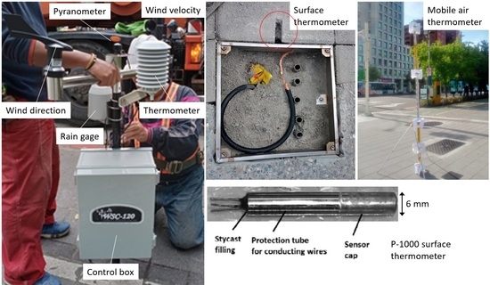
3. Methodology
3.1. Effect of Surface Water Content
3.2. Surface Temperature
3.3. Near-Surface Microclimate Temperature
4. Data Analyses Results
4.1. Data Summary
4.2. Effect of Surface Water Content
4.3. Surface Temperature
4.4. Near-Surface Microclimate Air Temperature
5. Discussion
6. Conclusions
Author Contributions
Funding
Institutional Review Board Statement
Informed Consent Statement
Data Availability Statement
Acknowledgments
Conflicts of Interest
References
- Climate Change: Global Temperature. Available online: https://www.climate.gov/news-features/understanding-climate/climate-change-global-temperature (accessed on 31 May 2022).
- Climate Change: Global Temperature Projections. Available online: https://www.climate.gov/news-features/understanding-climate/climate-change-global-temperature-projections (accessed on 9 June 2022).
- A Degree of Concern: Why Global Temperatures Matter. Available online: https://climate.nasa.gov/news/2878/a-degree-of-concern-why-global-temperatures-matter/ (accessed on 9 June 2022).
- Sea Level to Rise up to a Foot by 2050, Interagency Report Finds. Available online: https://www.jpl.nasa.gov/news/sea-level-to-rise-up-to-a-foot-by-2050-interagency-report-finds (accessed on 9 June 2022).
- Li, D.; Bou-zeid, E. Synergistic Interactions between Urban Heat Islands and Heat Waves: The Impact in Cities Is Larger than the Sum of Its Parts. J. Appl. Meteorol. Climatol. 2013, 52, 2051–2064. [Google Scholar] [CrossRef]
- Mirzaei, P.A. Recent challenges in modeling of urban heat island. Sustain. Cities Soc. 2015, 19, 200–206. [Google Scholar] [CrossRef]
- Yaghoobian, N.; Kleissl, J.; Paw, U.K.T. An Improved Three-Dimensional Simulation of the Diurnally Varying Street-Canyon Flow. Bound.-Layer Meteorol. 2014, 153, 251–276. [Google Scholar] [CrossRef]
- Heaviside, C.; Macintyre, H.; Vardoulakis, S. The Urban Heat Island: Implications for Health in a Changing Environment. Curr. Envir. Health Rpt. 2017, 4, 296–305. [Google Scholar] [CrossRef]
- Jenkins, K.; Hall, J.; Glenis, V.; Kilsby, C.; McCarthy, M.; Goodess, C.; Smith, D.; Malleson, N.; Birkin, M. Probabilistic spatial risk assessment of heat impacts and adaptations for London. Clim. Chang. 2014, 124, 105–117. [Google Scholar] [CrossRef]
- Li, X.; Zhou, Y.; Yu, S.; Jia, G.; Li, H.; Li, W. Urban heat island impacts on building energy consumption: A review of approaches and findings. Energy 2019, 174, 407–419. [Google Scholar] [CrossRef]
- Grimm, N.B.; Faeth, S.H.; Golubiewski, N.E.; Redman, C.L.; Wu, J.; Bai, X.; Briggs, J.M. Global Change and The Ecology of Cities. Science 2008, 319, 756–760. [Google Scholar] [CrossRef]
- Lai, D.; Liu, W.; Gan, T.; Liu, K.; Chen, Q. A review of mitigating strategies to improve the thermal environment and thermal comfort in urban outdoor spaces. Sci. Total Environ. 2019, 661, 337–353. [Google Scholar] [CrossRef]
- Jaafar, H.; Lakkis, I.; Yeretzian, A. Impact of boundary conditions in a microclimate model on mitigation strategies affecting temperature, relative humidity, and wind speed in a Mediterranean city. Build. Environ. 2022, 210, 108712. [Google Scholar] [CrossRef]
- Federal Highway Administration. Stormwater Best Management Practices in an Ultra-Urban Setting: Selection and Monitoring, Publication No. FHWA-EP-00-002; Office of Natural Environment, Federal Highway Administration: Washington, DC, USA, 2000.
- BMP Technical Design Manual, Volume III. Available online: https://www.maine.gov/dep/land/stormwater/stormwaterbmps/ (accessed on 9 June 2022).
- Qin, Y.; Hiller, J.E. Water availability near the surface dominates the evaporation of pervious concrete. Constr. Build. Mater. 2016, 111, 77–84. [Google Scholar] [CrossRef]
- Chatzidimitriou, A.; Yannas, S. Microclimate development in open urban spaces: The influence of form and materials. Energy Build. 2015, 108, 156–174. [Google Scholar] [CrossRef]
- Yaghoobian, N.; Kleissl, J. Effect of reflective pavements on building energy use. Urban Clim. 2012, 2, 25–42. [Google Scholar] [CrossRef]
- Dimoudi, A.; Kantzioura, A.; Zoras, S.; Pallas, C.; Kosmopoulos, P. Investigation of urban microclimate parameters in an urban center. Energy Build. 2013, 64, 1–9. [Google Scholar] [CrossRef]
- Yaghoobian, N.; Kleissl, J.; Krayenhoff, E.S. Modeling the Thermal Effects of Artificial Turf on the Urban Environment. J. Appl. Meteorol. Climatol. 2010, 49, 332–345. [Google Scholar] [CrossRef]
- Huang, L.; Li, J.; Zhao, D.; Zhu, J. A fieldwork study on the diurnal changes of urban microclimate in four types of ground cover and urban heat island of Nanjing, China. Build. Environ. 2008, 43, 7–17. [Google Scholar] [CrossRef]
- Chen, J.; Chu, R.; Wang, H.; Zhang, L.; Chen, X.; Du, Y. Alleviating urban heat island effect using high-conductivity permeable concrete pavement. J. Clean. Prod. 2019, 237, 117722. [Google Scholar] [CrossRef]
- Li, H.; Harvey, J.; Ge, Z. Experimental investigation on evaporation rate for enhancing evaporative cooling effect of permeable pavement materials. Constr. Build. Mater. 2014, 65, 367–375. [Google Scholar] [CrossRef]
- Wang, J.; Meng, Q.; Tan, K.; Zhang, L.; Zhang, Y. Experimental investigation on the influence of evaporative cooling of permeable pavements on outdoor thermal environment. Build. Environ. 2018, 140, 184–193. [Google Scholar] [CrossRef]
- Amani-Beni, M.; Chen, Y.; Vasileva, M.; Zhang, B.; Xie, G.-d. Quantitative-spatial relationships between air and surface temperature, a proxy for microclimate studies in fine-scale intra-urban areas? Sustain. Cities Soc. 2022, 77, 103584. [Google Scholar] [CrossRef]
- Stoll, M.J.; Brazel, A.J. Surface-air temperature relationships in the urban environment of Phoenix, Arizona. Phys. Geogr. 1992, 13, 160–179. [Google Scholar] [CrossRef]
- Thomson, M.C.; Garcia-Herrera, R.; Beniston, M. Seasonal Forecasts, Climate Change and Human Health; Springer: Berlin, Germany, 2008; Chapter 9. [Google Scholar]
- CWB Observation Data Inquire System. Available online: https://e-service.cwb.gov.tw/HistoryDataQuery/index.jsp (accessed on 25 May 2022).
- Ramalingam, R.; Boguhn, D.; Fillinger, H. Study of robust thin film PT-1000 temperature sensors for cryogenic process control applications. AIP Conf. Proc. 2014, 1573, 126. [Google Scholar]
- Discharge Tables. Available online: https://www.openchannelflow.com/weirs/weir-plates/discharge-tables (accessed on 25 May 2022).
- Taleghani, M.; Berardi, U. The Effect of Pavement Characteristics on Pedestrians’ Thermal Comfort in Toronto. Urban Clim. 2018, 24, 449–459. [Google Scholar] [CrossRef]
- Brown, R.A.; Borst, M. Quantifying evaporation in a permeable pavement system. Hydrol. Process. 2015, 29, 2100–2111. [Google Scholar] [CrossRef]
- Voogt, J.A.; Oke, T.R. Thermal remote sensing of urban climates. Remote Sens. Environ. 2003, 86, 370–384. [Google Scholar] [CrossRef]
- Battista, G.; Carnielo, E.; De Lieto Vollaro, R. Thermal impact of a redeveloped area on localized urban microclimate: A case study in Rome. Energy Build. 2016, 133, 446–454. [Google Scholar] [CrossRef]
- Chen, X.; Su, Z.; Ma, Y.; Yang, K.; Wang, B. Estimation of surface energy fluxes under complex terrain of Mt. Qomolangma over the Tibetan Plateau. Hydrol. Earth Syst. Sci. 2013, 17, 1607–1618. [Google Scholar] [CrossRef]
- Cayan, D. Latent and sensible heat flux anomalies over the Northern Oceans: Driving the sea surface temperature. J. Phys. Oceanogr. 1992, 22, 859–881. [Google Scholar] [CrossRef]
- Vapor Pressure. Available online: https://www.weather.gov/media/epz/wxcalc/vaporPressure.pdf (accessed on 10 May 2022).
- Chen, J.; Wang, H.; Xie, P. Pavement temperature prediction: Theoretical models and critical affecting factors. Appl. Therm. Eng. 2019, 158, 113755. [Google Scholar] [CrossRef]
- Hastie, T.; Tibshirani, R.; Friedman, J. The Elements of Statistical Learning: Data Mining, Inference and Prediction; Springer-Verlag: New York, NY, USA, 2001. [Google Scholar]
- Tu, M.-c.; Smith, P.; Filippi, A.M. Hybrid forward-selection method-based water-quality estimation via combining Landsat TM, ETM+, and OLI/TIRS images and ancillary environmental data. PLoS ONE 2018, 13, e0201255. [Google Scholar] [CrossRef] [PubMed]
- Gaffin, S.R.; Rosenzweig, C.; Khanbilvardi, R.; Parshall, L.; Mahani, S.; Glickman, H.; Goldberg, R.; Blake, R.; Slosberg, R.B.; Hillel, D. Variations in New York city’s urban heat island strength over time and space. Theor. Appl. Clim. 2008, 94, 1–11. [Google Scholar] [CrossRef]
- Loftus, G.R. On interpretation of interactions. Mem. Cogn. 2015, 6, 312–319. [Google Scholar] [CrossRef]
- Husain, S.Z.; Belair, S.; Leroyer, S. Influence of Soil Moisture on Urban Microclimate and Surface-Layer Meteorology in Oklahoma City. J. Appl. Meteorol. Climatol. 2014, 53, 83–98. [Google Scholar] [CrossRef]
- Tziampou, N.; Coupe, S.J.; Sanudo-Fontaneda, L.A.; Newman, A.P.; Castro-Fresno, D. Fluid transport within permeable pavement systems: A review of evaporation processes, moisture loss measurement and the current state of knowledge. Constr. Build. Mater. 2020, 243, 118179. [Google Scholar] [CrossRef]
- Shahrestani, M.; Yao, R.; Luo, Z.; Turkbeyler, E.; Davies, H. A field study of urban microclimates in London. Renew. Energy 2015, 73, 3–9. [Google Scholar] [CrossRef]
- Wang, J.; Meng, Q.; Tan, K.; Santamouris, M. Evaporative cooling performance estimation of pervious pavement based on evaporation resistance. Build. Environ. 2022, 217, 109083. [Google Scholar] [CrossRef]
- Kevern, J.T.; Haselbach, L.; Schaefer, V.R. Hot Weather Comparative Heat Balances in Pervious Concrete and Impervious Concrete Pavement Systems. J. Heat Isl. Inst. Int. 2012, 7, 231–237. [Google Scholar]
- Brotas, L.; Wilson, M. Daylight in urban canyons: Planning in Europe. In Proceedings of the PLEA 2006 The 23rd Conference on Passive and Low Energy Architecture, Geneva, Switzerland, 6–8 September 2006. [Google Scholar]
- Zhong, X.; Zhao, L.; Zhang, X.; Yan, J.; Ren, P. Investigating the effects of surface moisture content on thermal infrared emissivity of urban underlying surfaces. Constr. Build. Mater. 2022, 327, 127023. [Google Scholar] [CrossRef]
- Climate Science Investigations (CSI). Available online: http://www.ces.fau.edu/nasa/module-2/how-greenhouse-effect-works.php (accessed on 16 May 2022).
- Zhang, R.; Kuang, W.; Yang, S.; Li, Z. The influence of urban three-dimensional structure and building greenhouse effect on local radiation flux. Sci. China Earth Sci. 2021, 64, 1934–1948. [Google Scholar] [CrossRef]
- Gobel, P.; Starke, P.; Coldewey, W.G. Evaporation measurements on enhanced water-permeable paving in urban areas. In Proceedings of the 11th International Conference on Urban Drainage, Edinburgh, UK, 24–28 June 2008. [Google Scholar]
- Antoniou, N.; Montazeri, H.; Neophytou, M.; Blocken, B. CFD simulation of urban microclimate: Validation using high-resolution field measurements. Sci. Total Environ. 2019, 695, 133743. [Google Scholar] [CrossRef]
- Amnuaylojaroen, T.; Chanvichit, P. Projection of near-future climate change and agricultural drought in Mainland Southeast Asia under RCP8.5. Clim. Chang. 2019, 155, 175–193. [Google Scholar] [CrossRef]


| PT1000 Surface Temperature Sensor | ||
| Temperature | Range | −50–110 °C |
| Accuracy | ±1% | |
| Sampling interval | 5 min | |
| WSC-120 Weather Station | ||
| Temperature | Range | 0–60 °C |
| Accuracy | ±0.3 °C | |
| Humidity | Range | 0–100% RH |
| Accuracy | ±3% RH | |
| Wind speed | Range | 0–60 m/s |
| Accuracy | ± (0.3 + 0.03 wind speed) m/s | |
| Wind direction | Range | 0–360° |
| Accuracy | ±2° | |
| Rainfall | Accuracy | 1 mm |
| Sampling interval | 5 min | |
| JSQ-214 Pyranometer | ||
| Field of view | 180° | |
| Spectral range | 410–655 nm | |
| Calibration uncertainty | ±5% | |
| Sampling interval | 5 min | |
| SP-214-SS Pyranometer | ||
| Field of view | 180° | |
| Spectral range | 360–1120 nm | |
| Calibration uncertainty | ±3% | |
| Sampling interval | 5 min | |
| THD-8 Air Temperature and Humidity Sensor | ||
| Temperature | Range | −20–80 °C |
| Accuracy | ±0.3 °C | |
| Humidity | Range | 0–100% RH |
| Accuracy | ±2% RH | |
| Sampling interval | 5 s | |
| Symbol | Description |
|---|---|
| Wind speed (m/s) | |
| Ambient air temperature (°C) | |
| Solar radiation (in irradiance, kW/m2) | |
| x-hour antecedent mean ambient air temperature (°C) | |
| x-hour antecedent rainfall depth (mm) | |
| * | The interaction term of x-hour ambient air temperature and rainfall depth |
| Symbol | Description |
|---|---|
| Wind speed (m/s) | |
| Ambient air temperature (°C) | |
| Surface temperature | |
| Solar radiation (in irradiance, kW/m2) | |
| x-hour antecedent mean ambient air temperature (°C) | |
| x-hour antecedent rainfall depth (mm) | |
| The interaction term of x-hour air temperature and rainfall depth |
| Wind Speed (m/s) | Air Temp. (°C) | Relative Humidity (%) | Solar Radiation (kW/m2) | Surface Temp. (°C) | Air Temperature (°C) | |||||
|---|---|---|---|---|---|---|---|---|---|---|
| 0.05 m | 0.5 m | 1 m | 2 m | 3 m | ||||||
| Mean | 0.68 | 30.6 | 66 | 0.41 | 39.7 | 33.4 | 32.6 | 32.6 | 32.5 | 32.5 |
| 95% CI | (0, 9.25) | (24.5, 37.0) | (47, 85) | (0, 0.95) | (26.0, 52.6) | (24.7, 42.4) | (24.4, 41.3) | (24.2, 40.2) | (24.1, 40.5) | (24.2, 40.4) |
| Wind Speed (m/s) | Air Temp. (°C) | Relative Humidity (%) | Solar Radiation (kW/m2) | Surface Temp. (°C) | Air Temperature (°C) | |||||
|---|---|---|---|---|---|---|---|---|---|---|
| 0.05 m | 0.5 m | 1 m | 2 m | 3 m | ||||||
| Mean | 0.34 | 30.6 | 66 | 0.42 | 42.0 | 33.8 | 32.8 | 32.8 | 32.6 | 32.7 |
| 95% CI | (0, 6.38) | (24.2, 36.9 | (47, 84) | (0, 0.96) | (28.3, 56.4) | (24.8, 42.9) | (24.3, 40.6) | (24.1, 40.7) | (24.5, 40.3) | (24.9, 40.1) |
| Pervious Pavement Site | |||||||
| Model Terms for 0.05 m Temp. | Coefficient | p-Value | 95% CI | Model Terms for 0.5-m Temp. | Coefficient | p-Value | 95% CI |
| 0.0044 | 0.95 | (−0.15, 0.16) | −0.00039 | 0.99 | (−0.12, 0.12) | ||
| −0.028 | 0.25 | (−0.076, 0.020) | −0.024 | 0.23 | (−0.063, 0.015) | ||
| −0.040 | 0.0044 * | (−0.067, −0.013) | −0.031 | 0.0062 * | (−0.053, −0.0090) | ||
| Model Terms for 1 m Temp. | Coefficient | p-value | 95% CI | Model Terms for 1.8 m Temp. + | Coefficient | p-value | 95% CI |
| 0.0031 | 0.96 | (−0.12, 0.13) | 0.019 | 0.76 | (−0.10, 0.14) | ||
| −0.023 | 0.25 | (−0.063, 0.017) | −0.025 | 0.21 | (−0.064, 0.014) | ||
| −0.032 | 0.0063 * | (−0.054, −0.0092) | −0.023 | 0.041 * | (−0.045, −0.00098) | ||
| Model Terms for 1.9 m Temp. + | Coefficient | p−value | 95% CI | Model Terms for 2 m Temp. | Coefficient | p−value | 95% CI |
| 0.021 | 0.74 | (−0.10, 0.15) | 0.023 | 0.71 | (−0.10, 0.15) | ||
| −0.025 | 0.21 | (−0.064, 0.014) | −0.025 | 0.20 | (−0.064, 0.014) | ||
| −0.022 | 0.052 | (−0.044, 0.00016) | −0.021 | 0.065 | (−0.043, 0.0013) | ||
| Model Terms for 3 m Temp. | Coefficient | p-value | 95% CI | ||||
| 0.031 | 0.63 | (−0.094, 0.16) | |||||
| −0.027 | 0.18 | (−0.066, 0.013) | |||||
| −0.018 | 0.12 | (−0.040, 0.0044) | |||||
| Impervious Pavement Site | |||||||
| Model Terms for 0.05 m Temp. | Coefficient | p-value | 95% CI | Model Terms for 0.5 m Temp. | Coefficient | p-value | 95% CI |
| 0.065 | 0.40 | (−0.088, 0.22) | 0.043 | 0.47 | (−0.076, 0.16) | ||
| 0.026 | 0.38 | (−0.033, 0.086) | 0.023 | 0.32 | (−0.023, 0.069) | ||
| −0.033 | 0.028 * | (−0.063, 0.0037) | −0.025 | 0.030 * | (−0.048, −0.0025) | ||
| Model Terms for 0.7 m Temp. + | Coefficient | p-value | 95% CI | Model Terms for 0.8 m Temp. + | Coefficient | p-value | 95% CI |
| 0.057 | 0.35 | (−0.062, 0.18) | 0.063 | 0.29 | (−0.056, 0.18) | ||
| 0.023 | 0.32 | (−0.023, 0.069) | 0.023 | 0.33 | (−0.023, 0.069) | ||
| −0.023 | 0.047 * | (−0.046, 0.00030) | −0.022 | 0.059 | (−0.045, 0.00089) | ||
| Model Terms for 1 m Temp. | Coefficient | p-value | 95% CI | Model Terms for 2 m Temp. | Coefficient | p-value | 95% CI |
| 0.077 | 0.21 | (−0.044, 0.20) | 0.071 | 0.25 | (−0.049, 0.19) | ||
| 0.023 | 0.34 | (−0.024, 0.070) | 0.021 | 0.38 | (−0.026, 0.067) | ||
| −0.020 | 0.093 | (−0.043, 0.0034) | −0.017 | 0.17 | (−0.039, 0.0069) | ||
| Model Terms for 3 m Temp. | Coefficient | p-value | 95% CI | ||||
| 0.064 | 0.29 | (−0.055, 0.18) | |||||
| 0.022 | 0.34 | −0.024, 0.068) | |||||
| −0.017 | 0.14 | (−0.040, 0.0058) | |||||
| Pervious Surface (R2 = 0.81) | Impervious Surface (R2 = 0.84) | |||||||
|---|---|---|---|---|---|---|---|---|
| Term | p-Value | Coefficient | 95% CI | VIF | p-Value | Coefficient | 95% CI | VIF |
| 0.0005 * | 1.22 | (0.55, 1.88) | 8.04 | <0.0001 * | 1.25 | (0.67, 1.83) | 8.42 | |
| <0.0001 * | 12.56 | (8.27, 16.86) | 2.59 | <0.0001 * | 11.37 | (7.76, 14.98) | 2.70 | |
| 0.36 | −0.27 | (-0.85, 0.31) | 5.94 | 0.76 | −0.080 | (−0.61, 0.45) | 6.75 | |
| 0.31 | −0.043 | (−0.13, 0.040) | 1.06 | 0.74 | 0.015 | (−0.072, 0.10) | 1.22 | |
| + | 0.0004 * | −0.086 | (−0.13, −0.040) | 1.19 | 0.0012 * | −0.071 | (−0.11, −0.029) | 1.30 |
| Altitude | Term | Intercept | |||||
| 0.05 m (R2 = 0.95) | p-value | 0.076 | 0.090 | <0.0001 * | <0.0001 * | 0.11 | 0.058 |
| Coeff. | −2.20 | −0.095 | 1.00 | 0.23 | 1.26 | −0.17 | |
| 95% CI | (−4.64, 0.24) | (−0.21, 0.015) | (0.79, 1.22) | (0.17, 0.30) | (−0.29, 2.81) | (−0.35, 0.0062) | |
| VIF | - | 1.06 | 9.40 | 4.30 | 3.61 | 5.83 | |
| 0.5 m (R2 = 0.95) | p-value | 0.13 | - | <0.0001 * | <0.0001 * | 0.11 | 0.085 |
| Coeff. | −1.72 | - | 1.02 | 0.17 | 1.15 | −0.14 | |
| 95% CI | (−3.94, 0.50) | - | (0.82, 1.22) | (0.11, 0.23) | (−0.27, 2.58) | (−0.30, 0.020) | |
| VIF | - | - | 9.19 | 4.30 | 3.60 | 5.74 | |
| 1 m (R2 = 0.94) | p-value | 0.26 | - | <0.0001 * | <0.0001 * | 0.0018 * | - |
| Coeff. | −1.42 | - | 0.89 | 0.15 | 2.20 | - | |
| 95% CI | (3.92, 1.07) | - | (0.78, 1.00) | (0.084, 0.21) | (0.85, 3.55) | - | |
| VIF | - | - | 2.38 | 4.28 | 2.55 | - | |
| 2 m (R2 = 0.95) | p-value | 0.084 | - | <0.0001 * | 0.0004 * | 0.018 * | 0.065 |
| Coeff. | −2.03 | - | 1.10 | 0.11 | 1.81 | −0.16 | |
| 95% CI | (−4.35, 0.28) | - | (0.90, 1.31) | (0.053, 0.17) | (0.33, 3.29) | (−0.33, 0.0098) | |
| VIF | - | - | 9.19 | 4.30 | 3.60 | 5.74 | |
| 3 m (R2 = 0.95) | p-value | 0.086 | - | <0.0001 * | 0.0025 * | 0.0052 * | 0.064 |
| Coeff. | −2.02 | - | 1.13 | 0.094 | 2.14 | −0.16 | |
| 95% CI | (−4.33, 0.29) | - | (0.92, 1.33) | (0.034, 0.15) | (0.66, 3.62) | (−0.33, 0.0093) | |
| VIF | - | - | 9.19 | 4.30 | 3.60 | 5.74 |
| Altitude | Term | Intercept | |||||
| 0.05 m (R2 = 0.97) | p-value | <0.0001 * | <0.0001 * | <0.0001 * | 0.071 | 0.0008 * | 0.0045 * |
| Coeff. | −4.16 | 1.16 | 0.23 | 1.22 | −0.27 | 0.036 | |
| 95% CI | (−6.16, −2.16) | (0.97, 1.35) | (0.16, 0.29) | (−0.10, 2.54) | (−0.43, −0.12) | (0.011, 0.060) | |
| VIF | - | 9.73 | 5.58 | 4.05 | 6.41 | 1.08 | |
| 0.5 m (R2 = 0.97) | p-value | 0.0007 * | <0.0001 * | <0.0001 * | 0.0046 * | 0.016 * | 0.0066 * |
| Coeff. | −2.85 | 1.06 | 0.16 | 1.57 | −0.15 | 0.028 | |
| 95% CI | (−4.47, −1.23) | (0.91, 1.22) | (0.11, 0.21) | (0.50, 2.64) | (−0.28, −0.029) | (0.0080, 0.048) | |
| VIF | - | 9.73 | 5.58 | 4.05 | 6.41 | 1.08 | |
| 1 m (R2 = 0.97) | p-value | <0.0001 * | <0.0001 * | 0.0001 * | 0.0097 * | 0.026 * | 0.0089 * |
| Coeff. | −3.92 | 1.16 | 0.12 | 1.67 | −0.17 | 0.031 | |
| 95% CI | (−5.81, −2.02) | (0.98, 1.34) | (0.063, 0.18) | (0.42, 2.93) | (−0.31, −0.020) | (0.0081, 0.054) | |
| VIF | - | 9.73 | 5.58 | 4.05 | 6.41 | 1.08 | |
| 2 m (R2 = 0.96) | p-value | 0.0004 * | <0.0001 * | 0.0001 * | 0.0306 * | 0.020 * | 0.011 * |
| Coeff. | −3.65 | 1.16 | 0.13 | 1.44 | −0.18 | 0.032 | |
| 95% CI | (−5.62, −1.68) | (0.97, 1.34) | (0.064, 0.19) | (0.14, 2.75) | (−0.33, −0.030) | (0.0077, 0.056) | |
| VIF | - | 9.73 | 5.58 | 4.05 | 6.41 | 1.08 | |
| 3 m (R2 = 0.96) | p-value | 0.0019 * | <0.0001 * | <0.0001 * | 0.0213 * | 0.051 | 0.013 * |
| Coeff. | −3.21 | 1.11 | 0.13 | 1.55 | −0.15 | 0.031 | |
| 95% CI | (−5.20, −1.23) | (0.92, 1.30) | (0.068, 0.19) | (0.24, 2.87) | (−0.31, 0.00074) | (0.0066, 0.055) | |
| VIF | - | 9.73 | 5.58 | 4.05 | 6.41 | 1.08 |
Disclaimer/Publisher’s Note: The statements, opinions and data contained in all publications are solely those of the individual author(s) and contributor(s) and not of MDPI and/or the editor(s). MDPI and/or the editor(s) disclaim responsibility for any injury to people or property resulting from any ideas, methods, instructions or products referred to in the content. |
© 2023 by the authors. Licensee MDPI, Basel, Switzerland. This article is an open access article distributed under the terms and conditions of the Creative Commons Attribution (CC BY) license (https://creativecommons.org/licenses/by/4.0/).
Share and Cite
Tu, M.-c.; Chen, W.-j. Field Measurement of the Dynamic Interaction between Urban Surfaces and Microclimates in Humid Subtropical Climates with Multiple Sensors. Sensors 2023, 23, 9835. https://doi.org/10.3390/s23249835
Tu M-c, Chen W-j. Field Measurement of the Dynamic Interaction between Urban Surfaces and Microclimates in Humid Subtropical Climates with Multiple Sensors. Sensors. 2023; 23(24):9835. https://doi.org/10.3390/s23249835
Chicago/Turabian StyleTu, Min-cheng, and Wei-jen Chen. 2023. "Field Measurement of the Dynamic Interaction between Urban Surfaces and Microclimates in Humid Subtropical Climates with Multiple Sensors" Sensors 23, no. 24: 9835. https://doi.org/10.3390/s23249835