
Autonomous Trajectory Planning for Spray Painting on Complex Surfaces Based on a Point Cloud Model

Abstract
:1. Introduction
- It is a simple surface representation method;
- The area and the normal vector of each small triangle are known and can be used to represent the paint distribution on the entire surface;
- The triangulated surface is considered a single object.
- No geometrical information like edges;
- Mesh data are unorganized and more likely to present errors like overlapping facets or data loss during surface reconstruction.
- Achieving an accurate illustration of a component’s geometry, including solids, surfaces, splines, arcs, lines, points, and other features;
- Information about the material is included.
- Every feature is independent. The more complex the object, the more individual its features, making analysis more difficult;
- If the paint quality is to be evaluated, a mesh representation must be generated.
2. System Overview
- The trajectory is generated using only a point cloud as the workpiece’s geometrical information. The point cloud can be generated through 3D scanning or generated from a CAD model;
- An algorithm for generating spray-painting trajectories autonomously that achieve full coverage of a complex surface while keeping the paint film thickness within a given range;
- A trajectory-generation algorithm capable of addressing the challenges presented by complex surfaces like complex shapes, holes, cavities, irregular edges, and high roughness;
- The ability to handle workpieces in non-predefined orientations without the use of special fixtures or established positions;
- A simulation of paint thickness to validate the generated trajectory in a virtual environment and use this information to improve the spraying parameters as the paint flux.
3. Materials and Methods
3.1. Acquisition of the 3D Point Cloud
3.2. Point Cloud Preprocesing
3.3. Process of 3D Data Extraction
3.3.1. Use of 3D Principal Component Analysis (PCA)
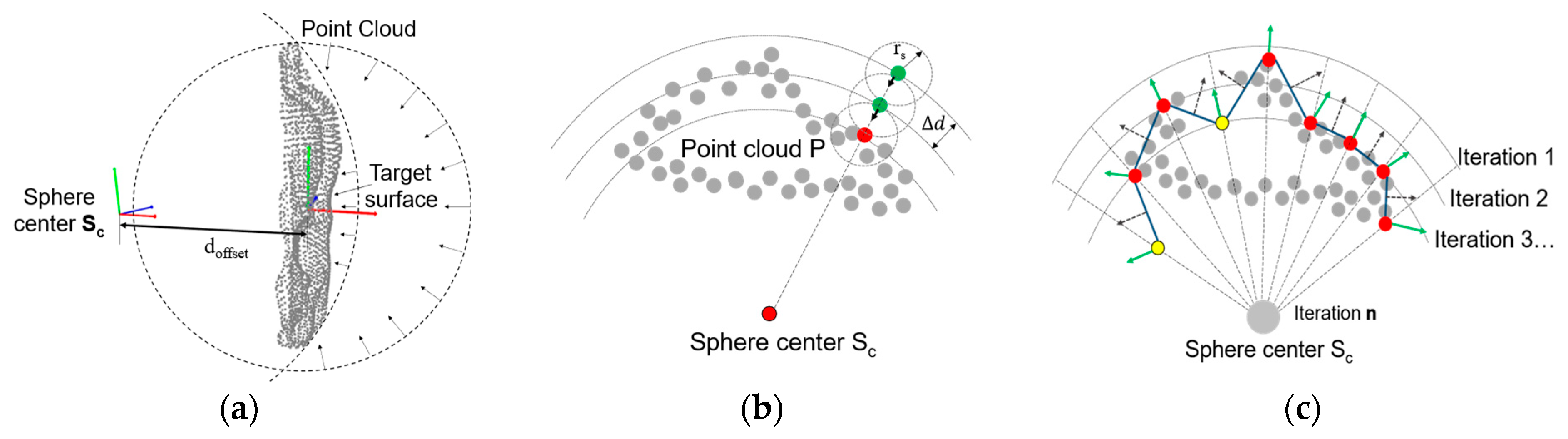
3.3.2. Spherical Mesh Grid Generation
3.3.3. Wrapping Method for Convex and Concave Surfaces


3.3.4. Surface Extraction and Preprocessing
4. Paint Deposition Model of Free-Form Surface
5. Path-Planning Algorithm
6. Robot Velocity Calculation
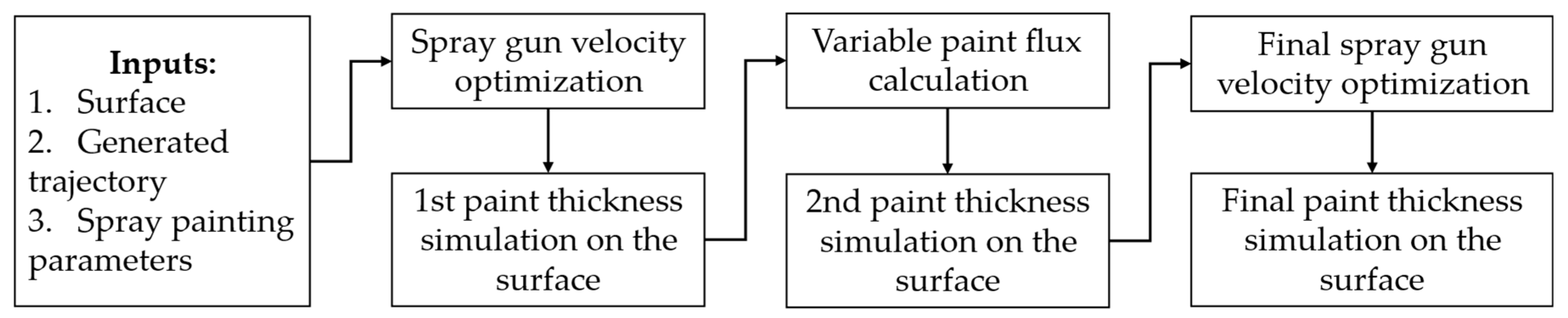
7. Variable Paint Flux Calculation
8. Simulation Results
9. Conclusions
Author Contributions
Funding
Institutional Review Board Statement
Data Availability Statement
Conflicts of Interest
References
- Boscariol, P.; Gasparetto, A.; Scalera, L. Path Planning for Special Robotic Operations. In Robot Design: From Theory to Service Applications; Carbone, G., Laribi, M.A., Eds.; Mechanisms and Machine Science; Springer International Publishing: Cham, Switzerland, 2023; pp. 69–95. [Google Scholar]
- Woods, A.; Pierson, H.A. Developing an ergonomic model and automation justification for spraying operations. In Proceedings of the IISE Annual Conference and Expo 2018, Orlando, FL, USA, 19–22 May 2018; pp. 293–298. [Google Scholar]
- Chen, W.; Wang, X.; Liu, H.; Tang, Y.; Liu, J. Optimized Combination of Spray Painting Trajectory on 3D Entities. Electronics 2019, 8, 74. [Google Scholar] [CrossRef]
- Chen, H.; Fuhlbrigge, T.; Li, X. Automated industrial robot path planning for spray painting process: A review. In Proceedings of the 2008 IEEE International Conference on Automation Science and Engineering, Washington, DC, USA, 23–26 August 2008; pp. 522–527. [Google Scholar]
- Weber, A.M.; Gambao, E.; Brunete, A. A Survey on Autonomous Offline Path Generation for Robot-Assisted Spraying Applications. Actuators 2023, 12, 403. [Google Scholar] [CrossRef]
- Andulkar, M.V.; Chiddarwar, S.S.; Marathe, A.S. Novel integrated offline trajectory generation approach for robot assisted spray painting operation. J. Manuf. Syst. 2015, 37, 201–216. [Google Scholar] [CrossRef]
- Cooper, I.; Nicholson, P.I.; Pierce, S.G.; Mineo, C. Introducing a novel mesh following technique for approximation-free robotic tool path trajectories. J. Comput. Des. Eng. 2017, 4, 192–202. [Google Scholar] [CrossRef]
- McGovern, S.; Xiao, J. A General Approach for Constrained Robotic Coverage Path Planning on 3D Freeform Surfaces. IEEE Trans. Autom. Sci. Eng. 2023, 20, 1–12. [Google Scholar] [CrossRef]
- Pan, Z.; Polden, J.; Larkin, N.; Van Duin, S.; Norrish, J. Recent progress on programming methods for industrial robots. Robot. Comput.-Integr. Manuf. 2012, 28, 87–94. [Google Scholar] [CrossRef]
- Bedaka, A.K.; Lin, C.-Y. CAD-based robot path planning and simulation using OPEN CASCADE. Procedia Comput. Sci. 2018, 133, 779–785. [Google Scholar] [CrossRef]
- Bedaka, A.K.; Mahmoud, A.M.; Lee, S.C.; Lin, C.Y. Autonomous Robot-Guided Inspection System Based on Offline Programming and RGB-D Model. Sensors 2018, 18, 4008. [Google Scholar] [CrossRef] [PubMed]
- Open Cascade. Available online: https://www.opencascade.com/ (accessed on 20 September 2023).
- Gleeson, D.; Jakobsson, S.; Salman, R.; Ekstedt, F.; Sandgren, N.; Edelvik, F.; Carlson, J.S.; Lennartson, B. Generating Optimized Trajectories for Robotic Spray Painting. IEEE Trans. Autom. Sci. Eng. 2022, 19, 1380–1391. [Google Scholar] [CrossRef]
- Chen, H.; Sheng, W.; Xi, N.; Song, M.; Chen, Y. Automated Robot Trajectory Planning for Spray Painting of Free-Form Surfaces in Automotive Manufacturing. Ind. Robot. Int. J. 2002, 29, 426–433. [Google Scholar] [CrossRef]
- Xu, Z.; He, W.; Yuan, K. A real-time position and posture measurement device for painting robot. In Proceedings of the 2011 International Conference on Electric Information and Control Engineering, ICEICE 2011—Proceedings, Wuhan, China, 15–17 April 2011; pp. 1942–1946. [Google Scholar] [CrossRef]
- Masood, A.; Siddiqui, R.; Pinto, M.; Rehman, H.; Khan, M.A. Tool Path Generation, for Complex Surface Machining, Using Point Cloud Data. Procedia CIRP 2015, 26, 397–402. [Google Scholar] [CrossRef]
- Wang, G.; Cheng, J.; Li, R.; Chen, K. A new point cloud slicing based path planning algorithm for robotic spray painting. In Proceedings of the 2015 IEEE International Conference on Robotics and Biomimetics, IEEE-ROBIO 2015, Zhuhai, China, 6–9 December 2015; pp. 1717–1722. [Google Scholar]
- Posada, J.R.D.; Meissner, A.; Hentz, G.; Agostino, N.D. Machine learning approaches for offline-programming optimization in robotic painting. In Proceedings of the ISR 2020; 52th International Symposium on Robotics, Online, 9–10 December 2020; pp. 1–7. [Google Scholar]
- Zhou, Q.-Y.; Park, J.; Koltun, V. Open3D: A Modern Library for 3D Data Processing. arXiv 2018, arXiv:1801.09847. [Google Scholar]
- Bowers, J.; Wang, R.; Maletz, D.; Wei, L.Y. Parallel Poisson Disk Sampling with Spectrum Analysis on Surfaces. ACM Trans. Graph. 2010, 29, 1–10. [Google Scholar] [CrossRef]
- Arcila, O.; Dinas, S.; Bañón, J.M. Collision detection model based on Bounding and containing Boxes. In Proceedings of the 2012 XXXVIII Conferencia Latinoamericana En Informatica (CLEI), Medellin, Colombia, 1–5 October 2012; pp. 1–10. [Google Scholar]
- Wang, Z.; Fan, J.; Jing, F.; Liu, Z.; Tan, M. A pose estimation system based on deep neural network and ICP registration for robotic spray painting application. Int. J. Adv. Manuf. Technol. 2019, 104, 285–299. [Google Scholar] [CrossRef]
- Chhay, S.; Adams, M.D. Visually aided feature extraction from 3D range data. In Proceedings of the 2010 IEEE International Conference on Robotics and Automation, Anchorage, Alaska, 3–8 May 2010; pp. 2273–2279. [Google Scholar]
- Lin, C.-H.; Chen, J.-Y.; Su, P.-L.; Chen, C.-H. Eigen-feature analysis of weighted covariance matrices for LiDAR point cloud classification. ISPRS J. Photogramm. Remote Sens. 2014, 94, 70–79. [Google Scholar] [CrossRef]
- Antonio, J.K. Optimal trajectory planning for spray coating. In Proceedings of the IEEE International Conference on Robotics and Automation, San Diego, CA, USA, 8–13 May 1994; pp. 2570–2577. [Google Scholar] [CrossRef]
- Freund, E.; Rokossa, D.; Rossmann, J. Process-oriented approach to an efficient off-line programming of industrial robots. IECON Proc. (Ind. Electron. Conf.) 1998, 1, 208–213. [Google Scholar] [CrossRef]
- Chen, H.; Xi, N.; Sheng, W.; Chen, Y. General framework of optimal tool trajectory planning for free-form surfaces in surface manufacturing. J. Manuf. Sci. Eng. 2005, 127, 49–59. [Google Scholar] [CrossRef]
- Sahir Arikan, M.A.; Engelberger, J.F.; Balkan, T. Modeling of paint flow rate flux for elliptical paint sprays by using experimental paint thickness distributions. Ind. Robot. Int. J. 2006, 33, 60–66. [Google Scholar] [CrossRef]
- Fogliati, M.; Fontana, D.; Garbero, M.; Vanni, M.; Baldi, G.; Dondè, R. CFD simulation of paint deposition in an air spray process. J. Coat. Technol. Res. 2006, 3, 117–125. [Google Scholar] [CrossRef]
- Wang, Z.; Liu, C.; Cheng, L.; Fan, X. Optimization of spraying path overlap rate based on MATLAB. In Proceedings of the 2012 2nd International Conference on Consumer Electronics, Communications and Networks, CECNet 2012—Proceedings, Yichang, China, 21–23 April 2012; Volume 1, pp. 2731–2734. [Google Scholar] [CrossRef]
- Yu, S.; Cao, L. Modeling and prediction of paint film deposition rate for robotic spray painting. In Proceedings of the 2011 IEEE International Conference on Mechatronics and Automation, ICMA 2011, Beijing, China, 7–10 August 2011; pp. 1445–1450. [Google Scholar] [CrossRef]
- Andulkar, M.V.; Chiddarwar, S.S.; Paigwar, A.K. Optimal velocity trajectory generation for spray painting robot in offline mode. In Proceedings of the 2015 Conference on Advances in Robotics, Goa, India, 2–4 July 2015; pp. 1–6. [Google Scholar]
- SSPC. SSPC-PA 2 Procedure for Determining Conformance to Dry Coating Thickness Requirements; Society for Protective Coatings Paint Application Standard: Houston, TX, USA, 2015; pp. 1–4. [Google Scholar]
- Trigatti, G.; Boscariol, P.; Scalera, L.; Pillan, D.; Gasparetto, A. A Look-Ahead Trajectory Planning Algorithm for Spray Painting Robots with Non-spherical Wrists. In Mechanism Design for Robotics: Proceedings of the 4th IFToMM Symposium on Mechanism Design for Robotics, Udine, Italy, 11–13 September 2018; Springer International Publishing: Cham, Switzerland, 2018; pp. 235–242. [Google Scholar]
- Görner, M.; Haschke, R.; Ritter, H.; Zhang, J. MoveIt! Task Constructor for Task-Level Motion Planning. In Proceedings of the 2019 International Conference on Robotics and Automation (ICRA), Montreal, QC, Canada, 20–24 May 2019; pp. 190–196. [Google Scholar]
- Koubâa, A. Robot Operating System (ROS); Polish Academy of Sciences: Warsaw, Poland, 2017; Volume 1. [Google Scholar]


| Input Parameters | Output Parameters |
|---|---|
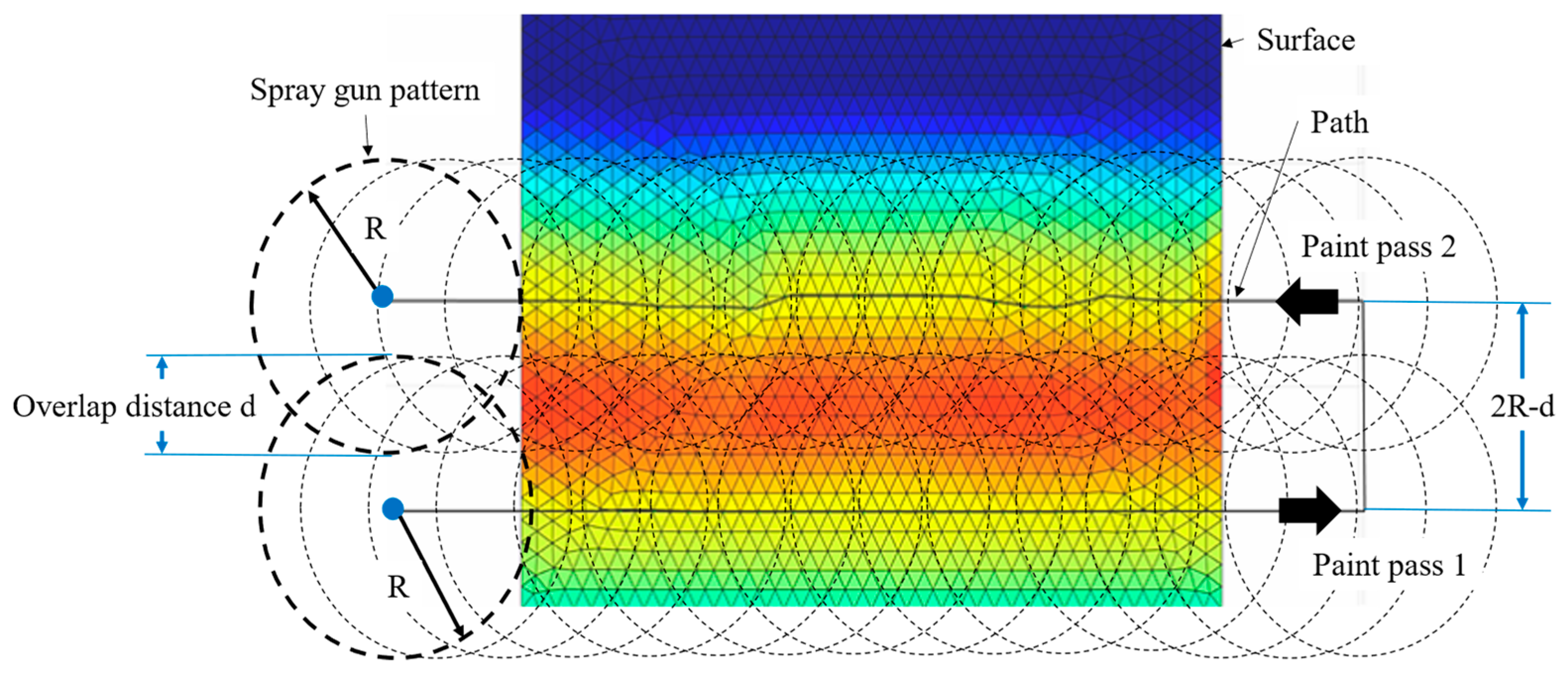
| Paint flux Q | Radius of spray circle R |
| Desired thickness qd | Overlap distance d |
| Allowed thickness variation qs | Spray-gun velocity v |
| Value β | |
| Spray-gun efficiency η | |
| Spray-gun angle θ | |
| Spray-gun standoff h |
| Input Parameters | Output Parameters |
|---|---|
| Paint flux Q (max) | 1000 mm3/s |
| Desired thickness qd | 0.025 mm |
| Allowed thickness variation qs | −20%/+50% |
| Value β | 2 |
| Spray-gun angle θ | 20° |
| Spray-gun efficiency η | 1 |
| Spray-gun standoff h | 100 mm |
| Velocity (mm/s) | Average Thickness (mm) | Thickness within the Allowed Variation (%) | Surface Coverage (%) | ||||
|---|---|---|---|---|---|---|---|
| Bellow Range | Inside Range | Above Range | |||||
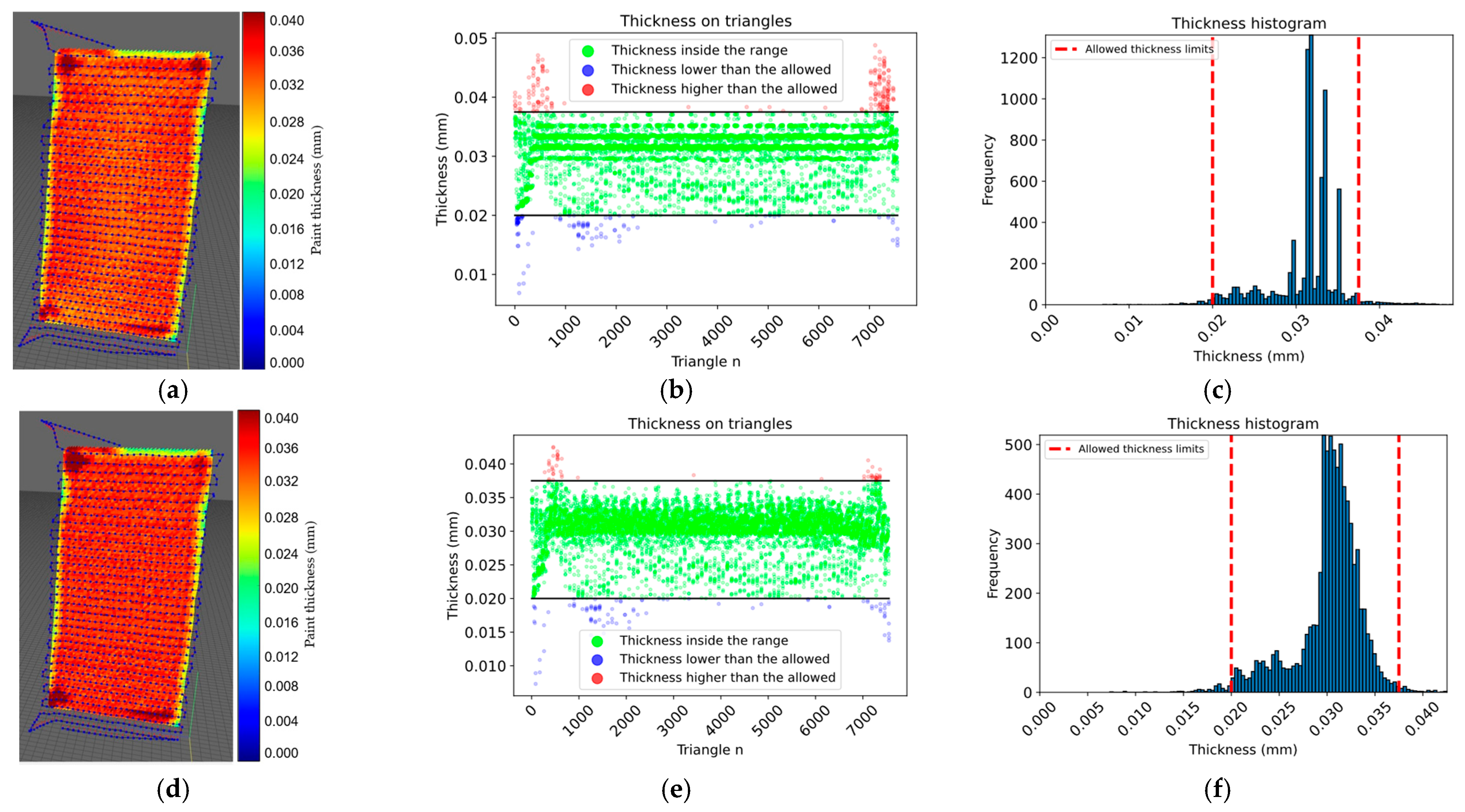
| Planar surface | Constant flux | 246.72 | 0.0312 | 1.53 | 96.08 | 2.37 | 100 |
| Variable flux | 255.49 | 0.0301 | 1.27 | 98.01 | 0.71 | ||
| Convex Surface | Constant flux | 454.06 | 0.0280 | 4.04 | 93.18 | 2.77 | 100 |
| Variable flux | 379.15 | 0.0289 | 2.16 | 97.45 | 0.37 | ||
| Motorbike engine cover | Constant flux | 585.83 | 0.0285 | 4.12 | 94.20 | 1.67 | 99.98 |
| Variable flux | 516.41 | 0.0290 | 2.37 | 96.63 | 0.98 | ||
| Transmission cover | Constant flux | 523.60 | 0.0259 | 18.06 | 73.68 | 8.25 | 96.65 |
| Variable flux | 551.72 | 0.0255 | 15.12 | 81.33 | 3.54 | ||
Disclaimer/Publisher’s Note: The statements, opinions and data contained in all publications are solely those of the individual author(s) and contributor(s) and not of MDPI and/or the editor(s). MDPI and/or the editor(s) disclaim responsibility for any injury to people or property resulting from any ideas, methods, instructions or products referred to in the content. |
© 2023 by the authors. Licensee MDPI, Basel, Switzerland. This article is an open access article distributed under the terms and conditions of the Creative Commons Attribution (CC BY) license (https://creativecommons.org/licenses/by/4.0/).
Share and Cite
Nieto Bastida, S.; Lin, C.-Y. Autonomous Trajectory Planning for Spray Painting on Complex Surfaces Based on a Point Cloud Model. Sensors 2023, 23, 9634. https://doi.org/10.3390/s23249634
Nieto Bastida S, Lin C-Y. Autonomous Trajectory Planning for Spray Painting on Complex Surfaces Based on a Point Cloud Model. Sensors. 2023; 23(24):9634. https://doi.org/10.3390/s23249634
Chicago/Turabian StyleNieto Bastida, Saul, and Chyi-Yeu Lin. 2023. "Autonomous Trajectory Planning for Spray Painting on Complex Surfaces Based on a Point Cloud Model" Sensors 23, no. 24: 9634. https://doi.org/10.3390/s23249634