Figure 1.
Overview of the system workflow. (The collected human activity data are processed and then classified before utilizing the XR-KS model).
Figure 1.
Overview of the system workflow. (The collected human activity data are processed and then classified before utilizing the XR-KS model).
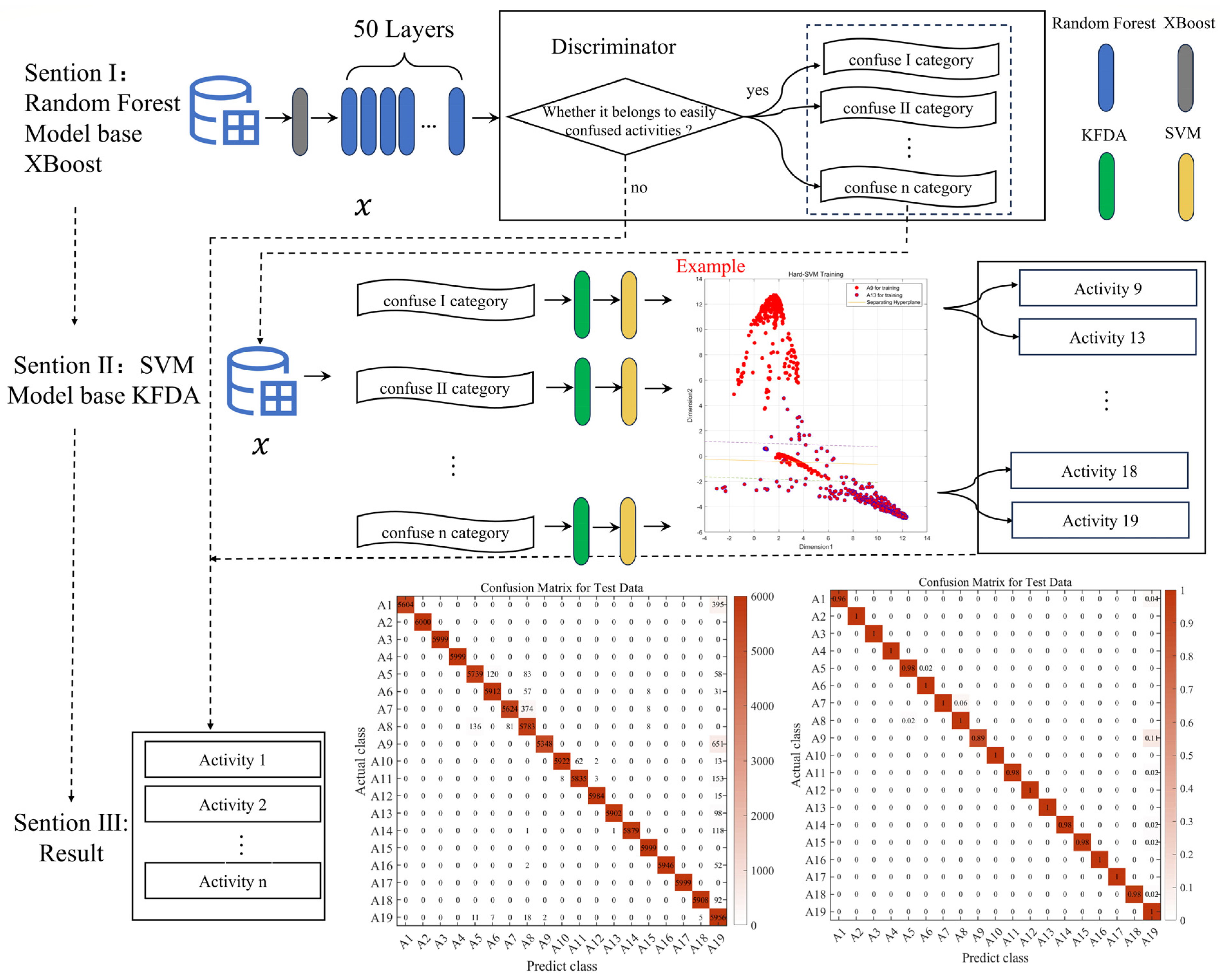
Figure 2.
XR-KS model workflow diagram. (The architecture of XR-KS. The first layer of this model relies on a random forest model based on the XGBoost feature selection algorithm, and then, based on the results of the first layer, the second layer uses the support vector machine model based on kernel Fisher discriminant analysis to output the final result, which is very effective in classifying similar human activities).
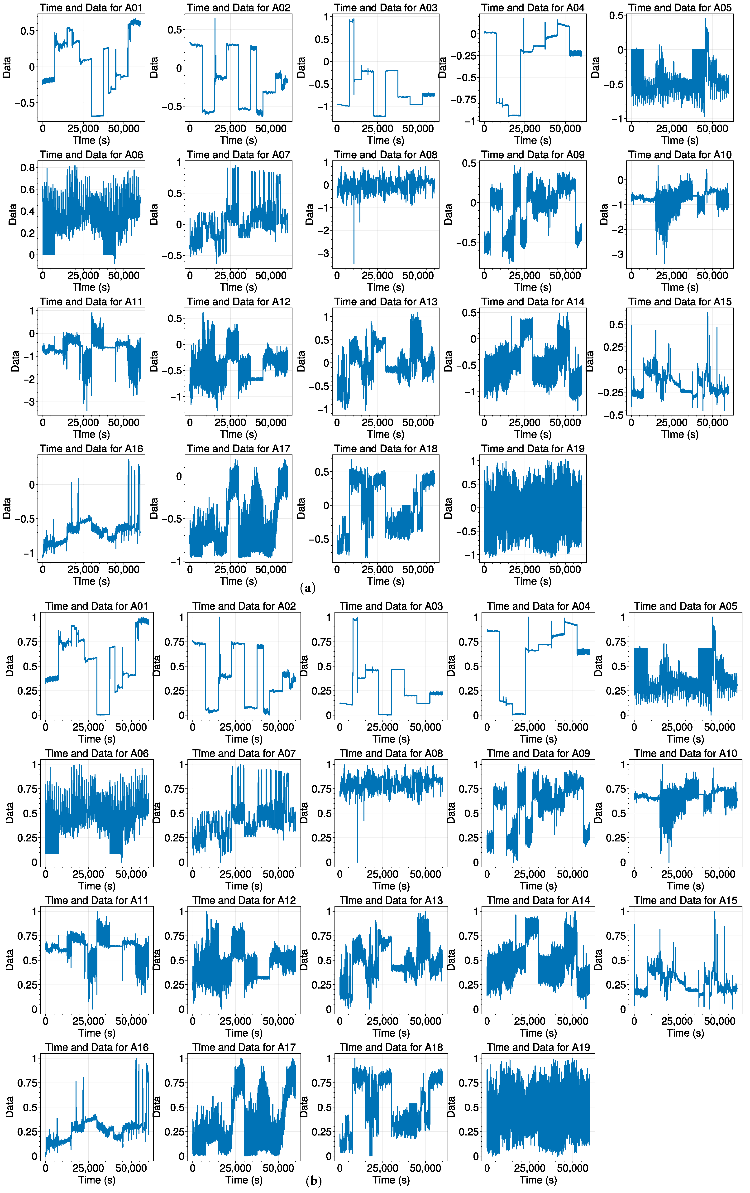
Figure 3.
Pre- and post-data preprocessed from A1 to A19. (Minimizing and normalizing aim to scale data consistently, ensuring equal influence from variables in the model). (a) Original data; (b) data after preprocessing.
Figure 3.
Pre- and post-data preprocessed from A1 to A19. (Minimizing and normalizing aim to scale data consistently, ensuring equal influence from variables in the model). (a) Original data; (b) data after preprocessing.
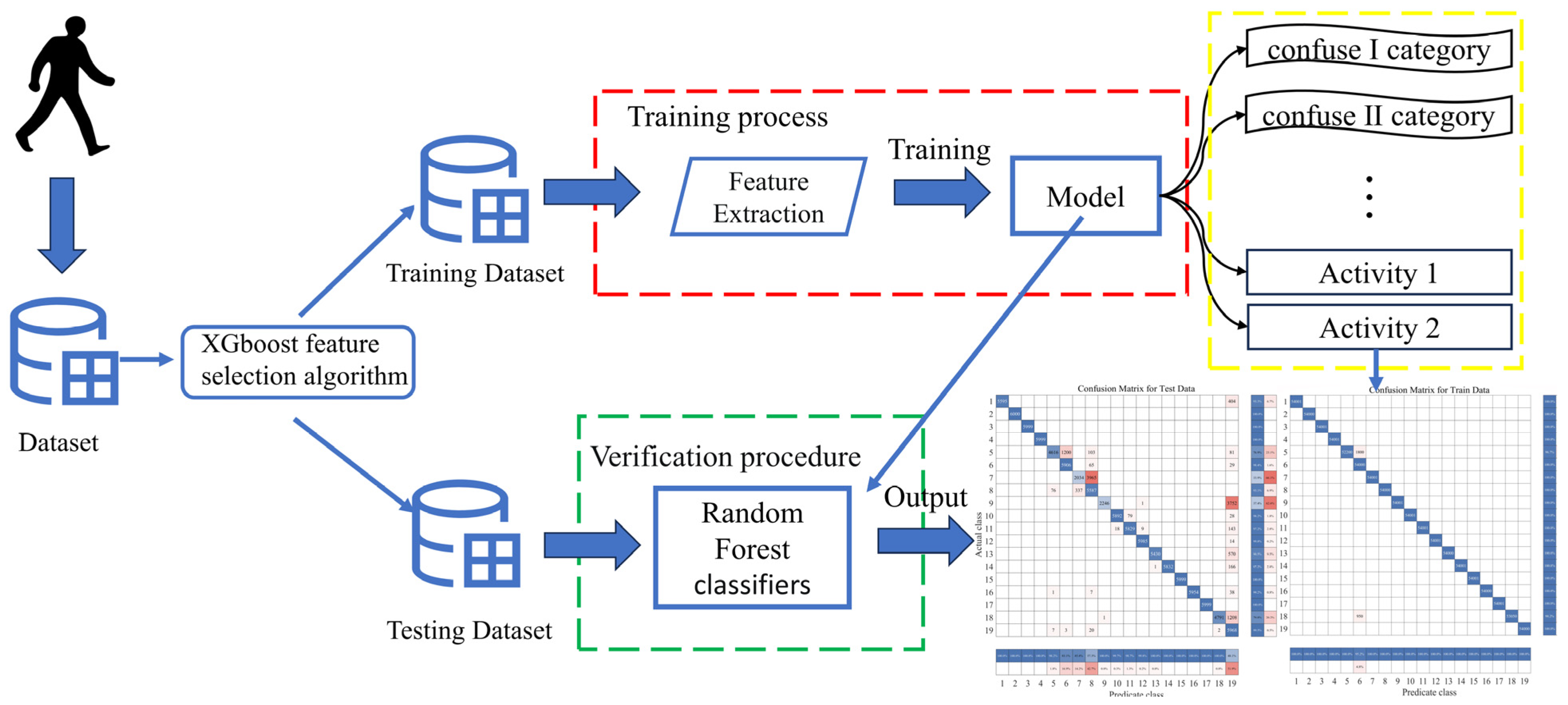
Figure 4.
Presentation of the random forest model based on the XGBoost feature selection algorithm workflow.
Figure 4.
Presentation of the random forest model based on the XGBoost feature selection algorithm workflow.
Figure 5.
Random forest algorithm flow chart.
Figure 5.
Random forest algorithm flow chart.
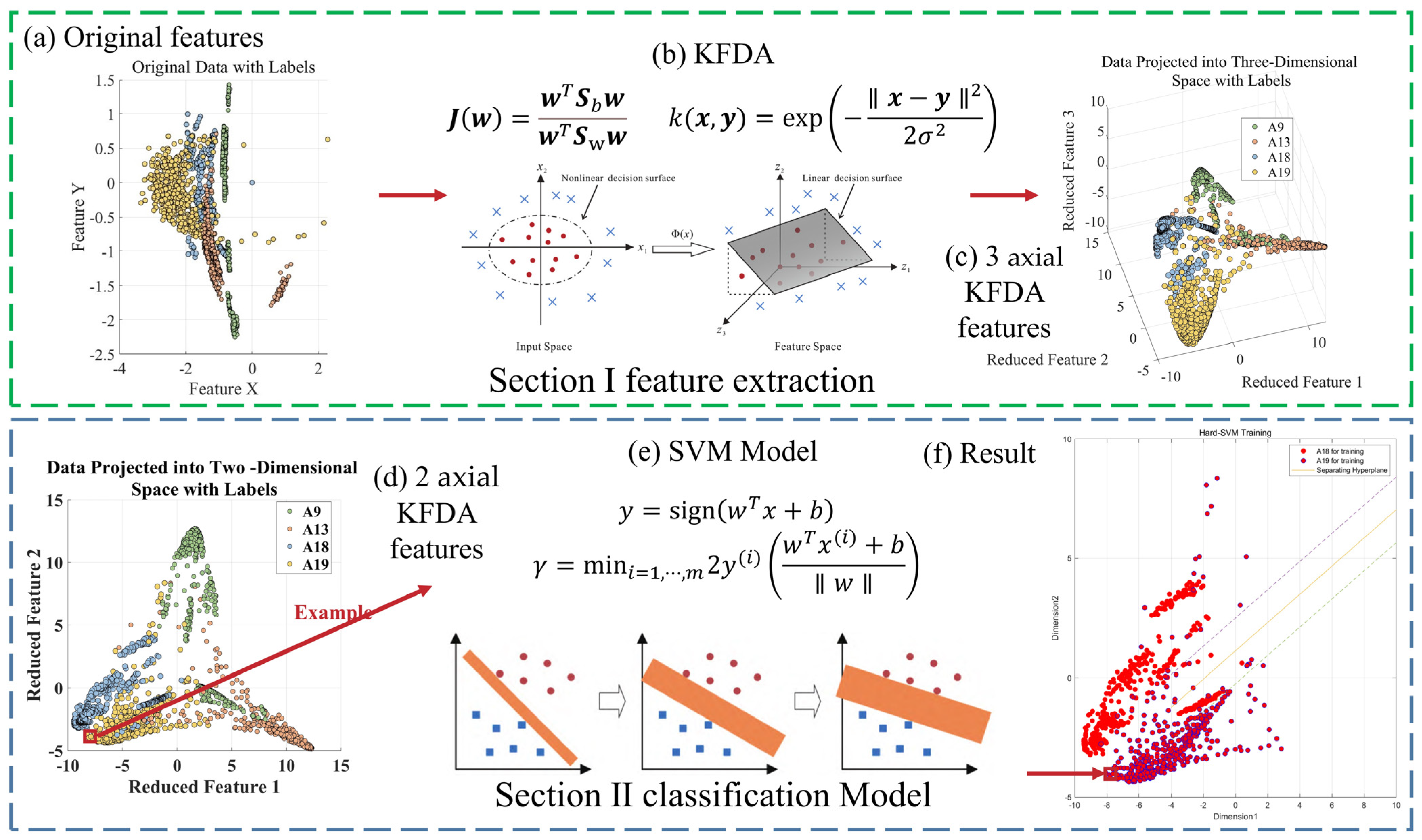
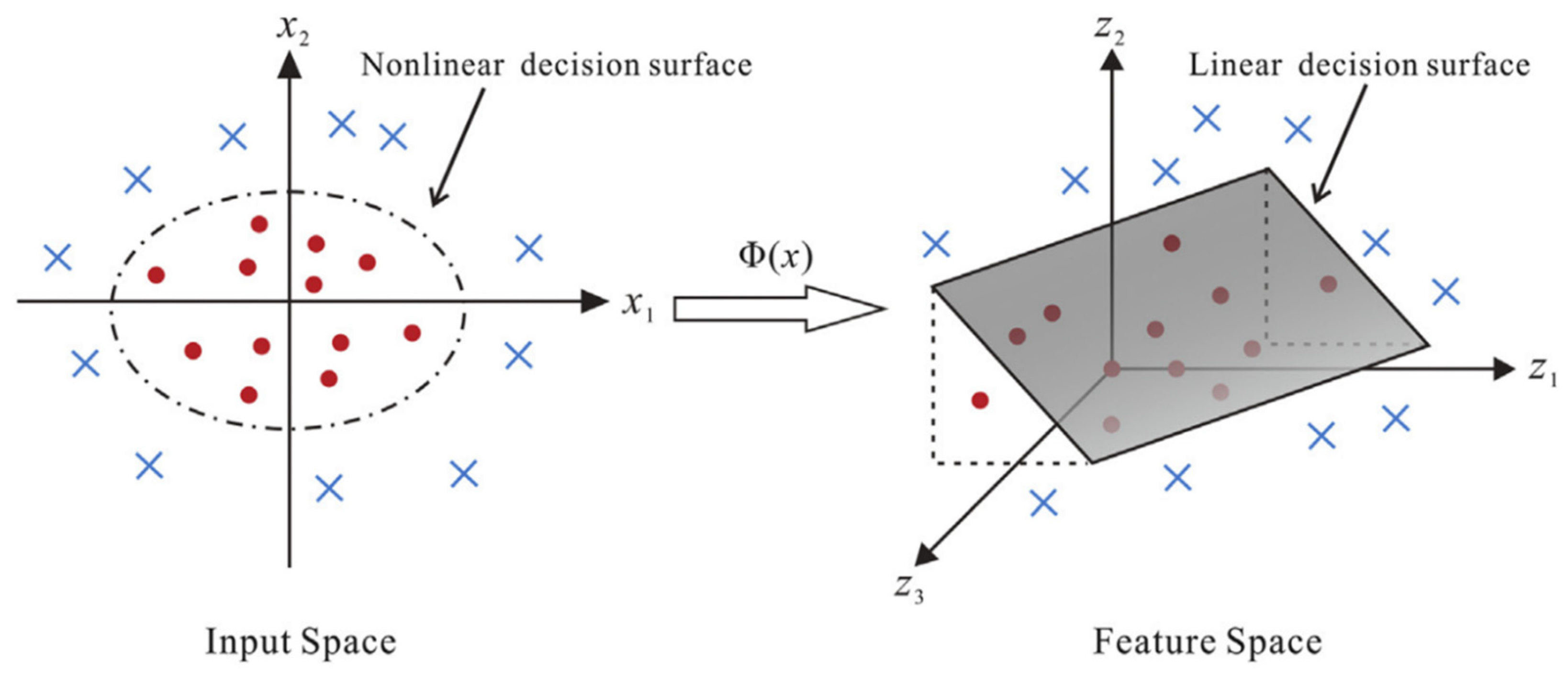
Figure 10.
Transformation process illustration of a KFD model. A nonlinear mapping function
converts a nonlinear problem in the original (low-dimensional) input space to a linear problem in a (higher-dimensional) feature space (from [
27]).
Figure 10.
Transformation process illustration of a KFD model. A nonlinear mapping function
converts a nonlinear problem in the original (low-dimensional) input space to a linear problem in a (higher-dimensional) feature space (from [
27]).
Figure 11.
Result of kernel Fisher discriminant analysis with varying parameters. (a) ; (b) ; (c) ; (d) ; (e) ; (f) .
Figure 11.
Result of kernel Fisher discriminant analysis with varying parameters. (a) ; (b) ; (c) ; (d) ; (e) ; (f) .
Figure 12.
Vector machine classification flow chart. (The figure displays blue and red dots representing distinct classes, with the SVM iteratively seeking the optimal classification hyperplane through continuous refinement).
Figure 12.
Vector machine classification flow chart. (The figure displays blue and red dots representing distinct classes, with the SVM iteratively seeking the optimal classification hyperplane through continuous refinement).
Figure 13.
Vector machine classification schematic.(different colors show positive and negative samples. Hollow circles mark support vectors, the points closest to the separating hyperplane. Solid markers represent instances farther away from the hyperplane)..
Figure 13.
Vector machine classification schematic.(different colors show positive and negative samples. Hollow circles mark support vectors, the points closest to the separating hyperplane. Solid markers represent instances farther away from the hyperplane)..
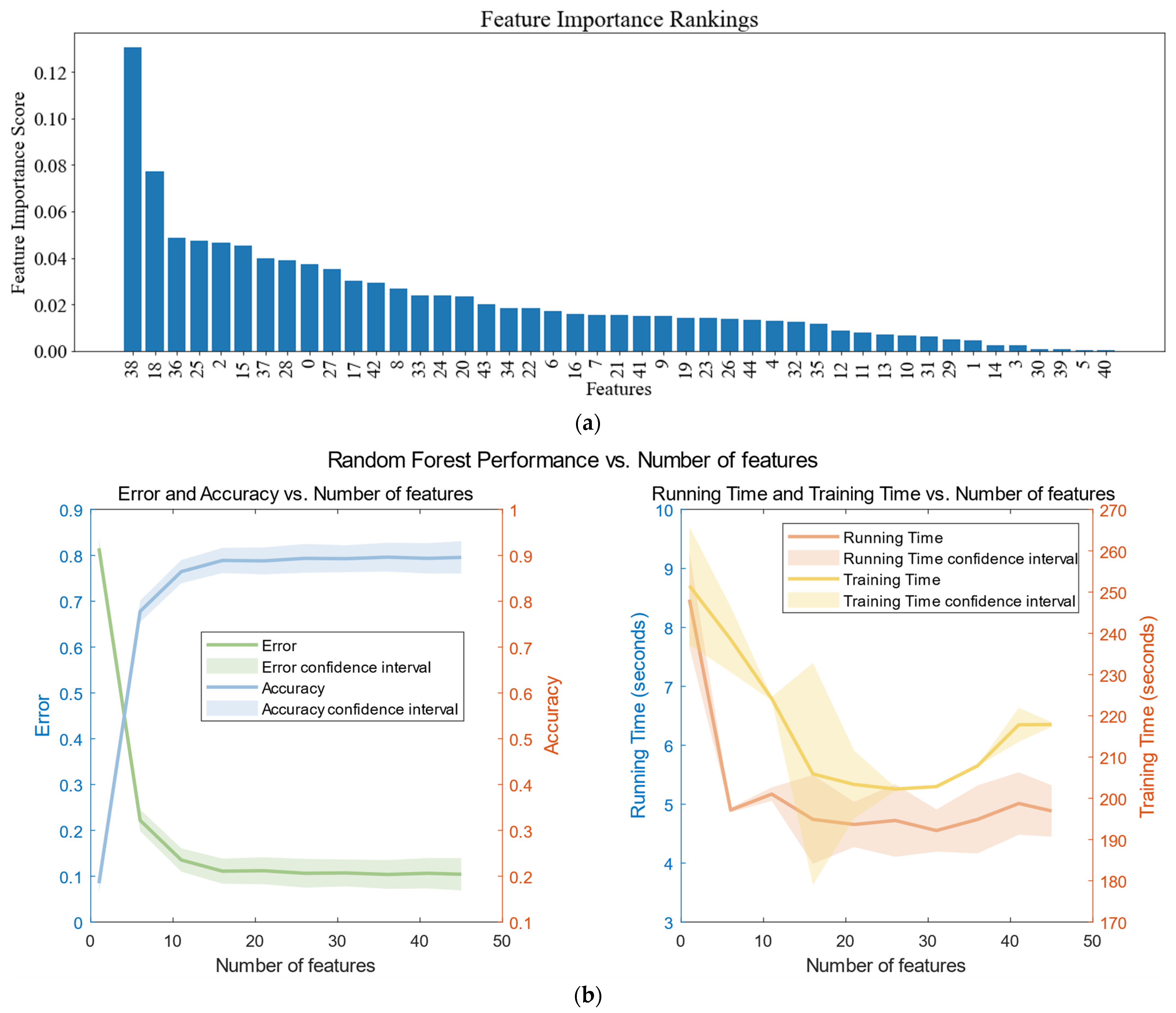
Figure 14.
Weights of important features chart and effect of different numbers of features on a random model. (We set the number of features to be from 1 to 46 steps, took 5, and repeated the error experiment for each different n to obtain the mean and confidence interval). (a) Result of the XGBoost feature value selection algorithm; (b) effect of different numbers of features on a random model.
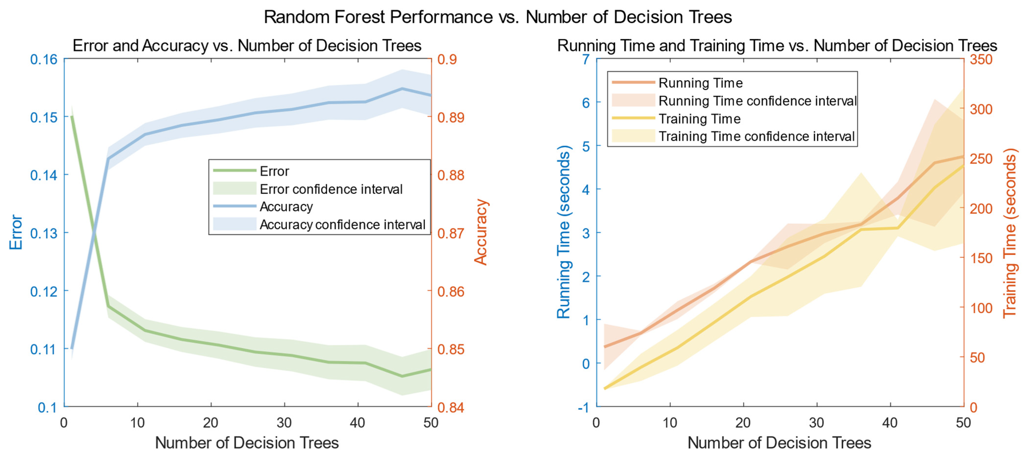
Figure 15.
Plot of the number of decisions versus error in the random forest model. (We set the number of decision trees to be from 1 to 50 steps, took 5, and repeated the error experiment for each different n to obtain the mean and confidence interval).
Figure 15.
Plot of the number of decisions versus error in the random forest model. (We set the number of decision trees to be from 1 to 50 steps, took 5, and repeated the error experiment for each different n to obtain the mean and confidence interval).
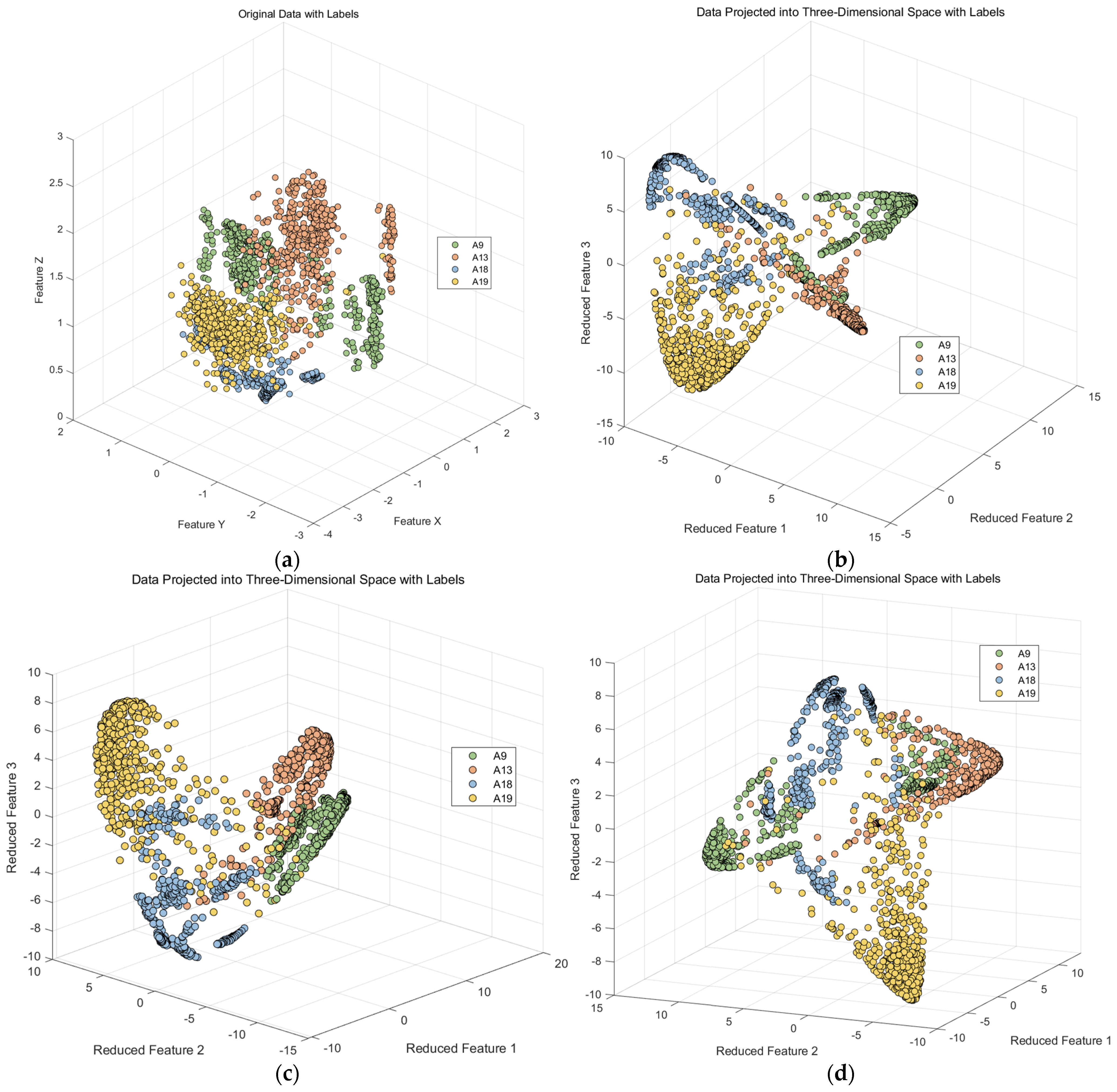
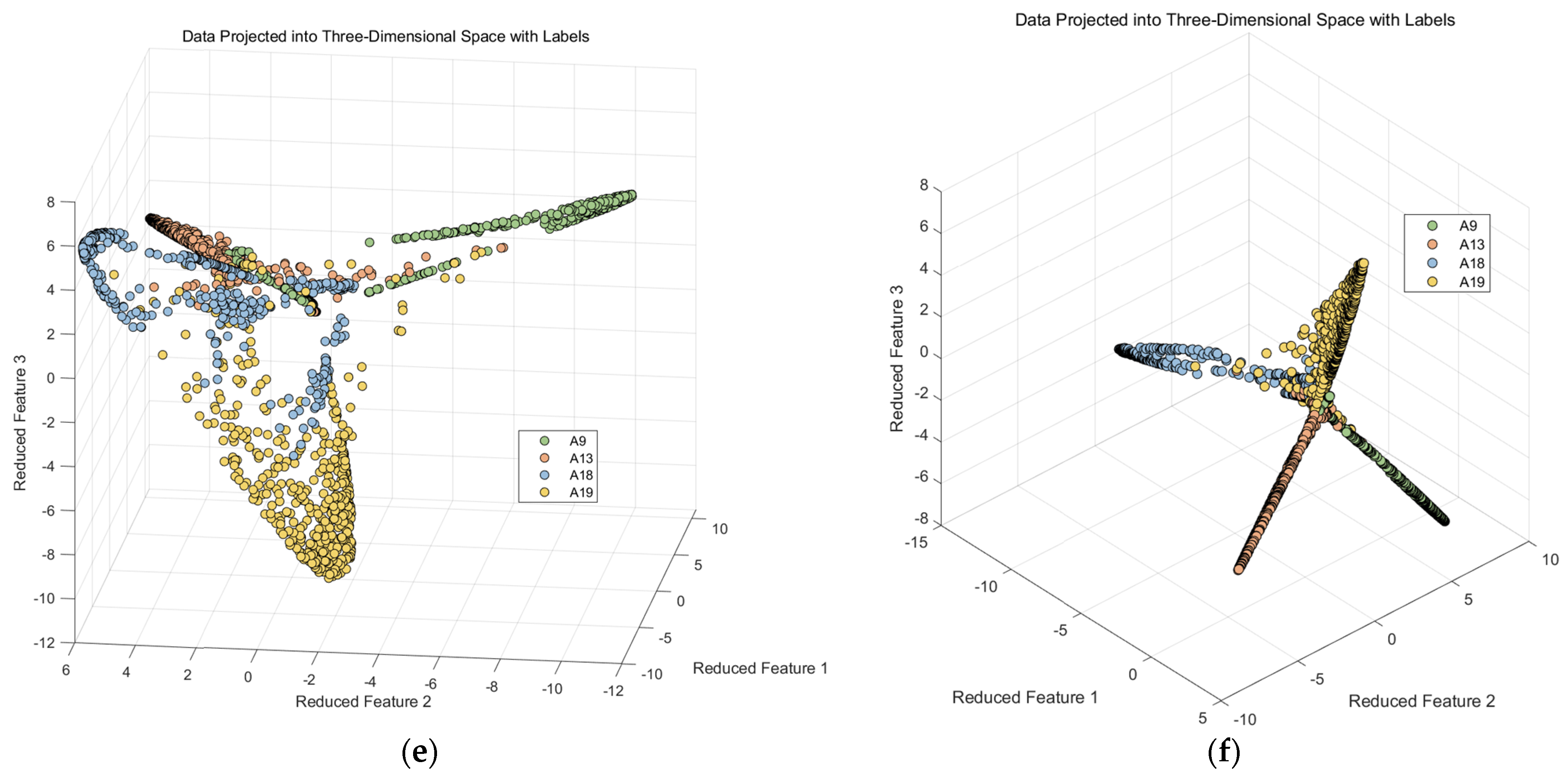
Figure 16.
Kernel Fisher discriminant analysis feature. (a) 3-axial of data; (b) 2-axial of data.
Figure 16.
Kernel Fisher discriminant analysis feature. (a) 3-axial of data; (b) 2-axial of data.
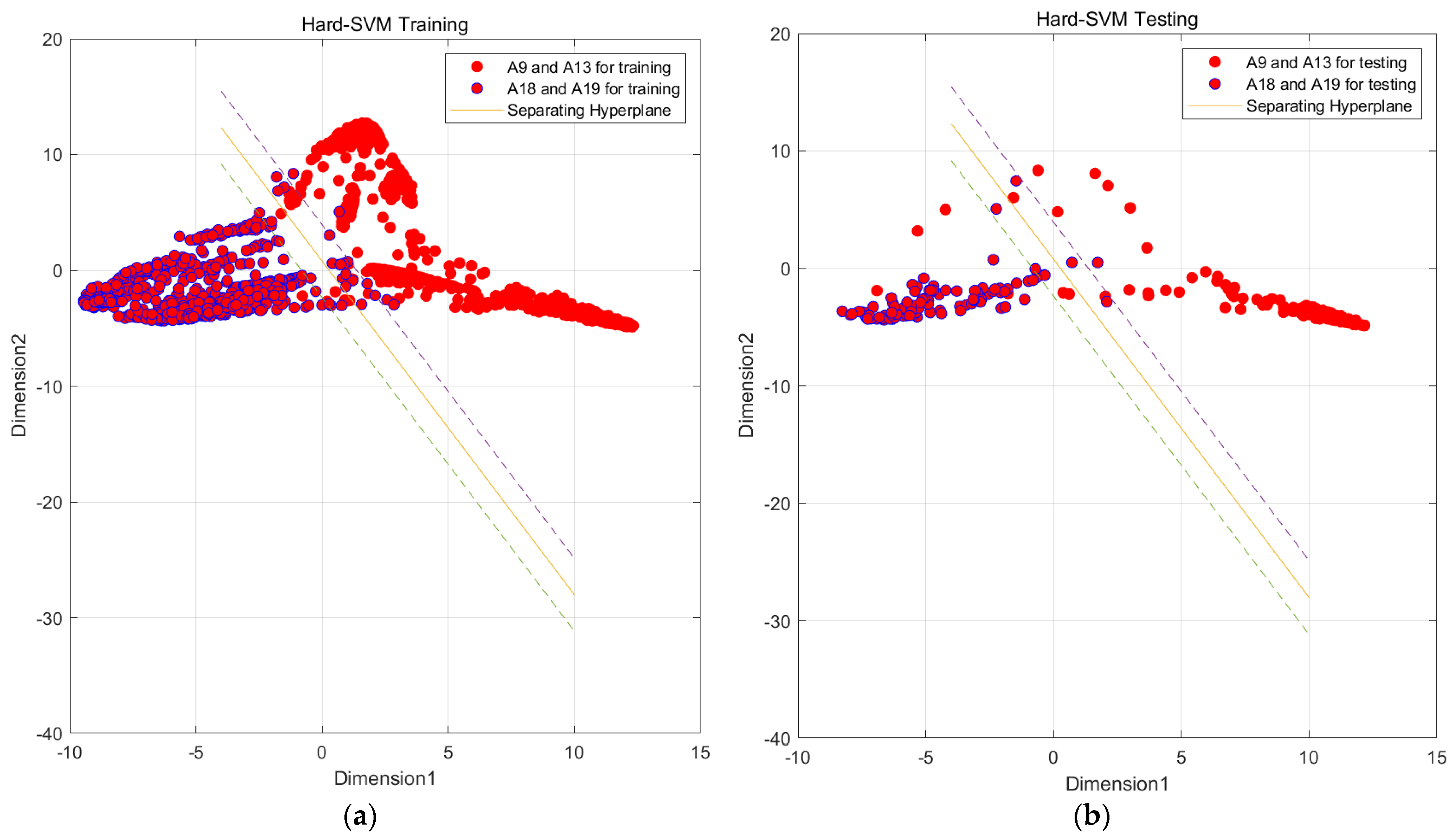
Figure 17.
SVM preliminary segmentation A9, A13 and A18, A19 result graph. (Solid line is the main decision boundary, and dashed line is the margin). (a) SVM model by train set; (b) SVM model by test set.
Figure 17.
SVM preliminary segmentation A9, A13 and A18, A19 result graph. (Solid line is the main decision boundary, and dashed line is the margin). (a) SVM model by train set; (b) SVM model by test set.
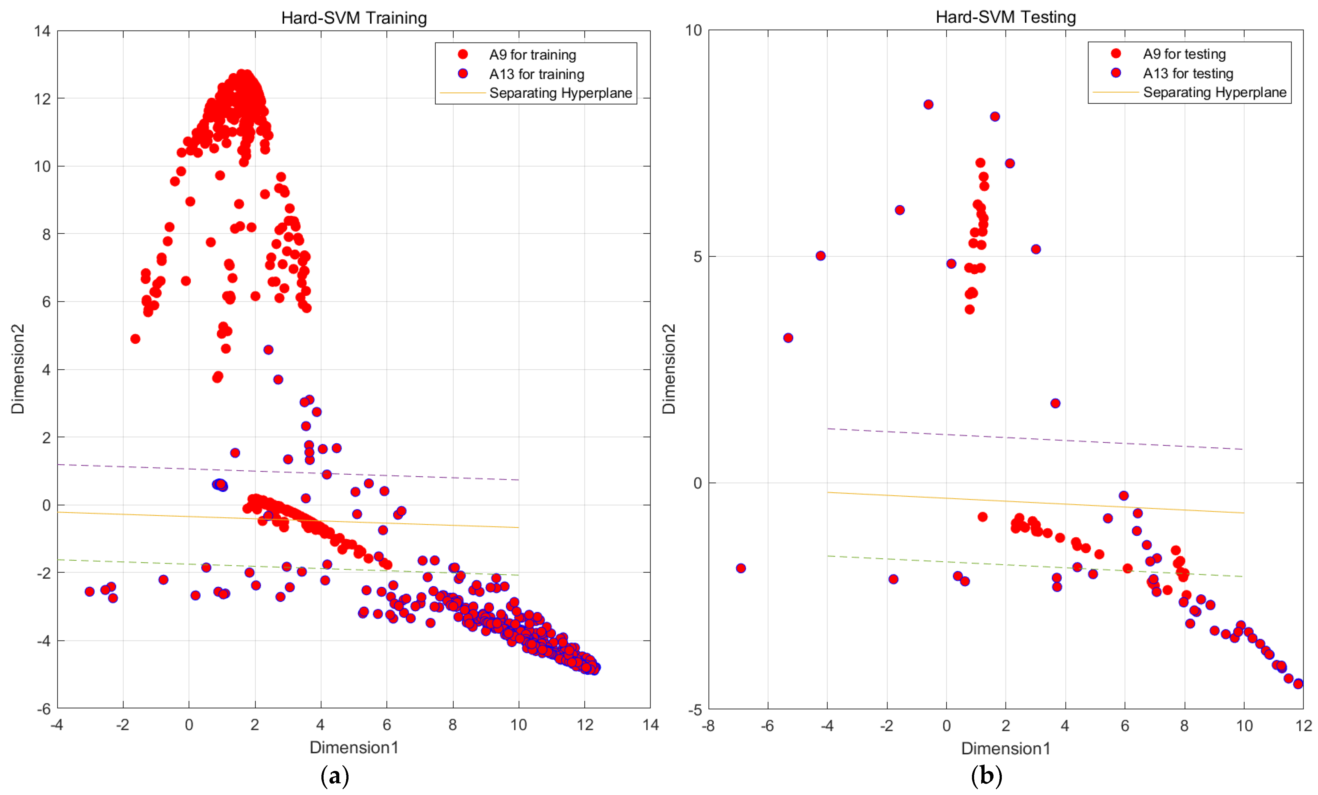
Figure 18.
SVM preliminary segmentation A9 and A13 result graph. (Solid line is the main decision boundary, and dashed line is the margin). (a) SVM model by train set; (b) SVM model by test set.
Figure 18.
SVM preliminary segmentation A9 and A13 result graph. (Solid line is the main decision boundary, and dashed line is the margin). (a) SVM model by train set; (b) SVM model by test set.
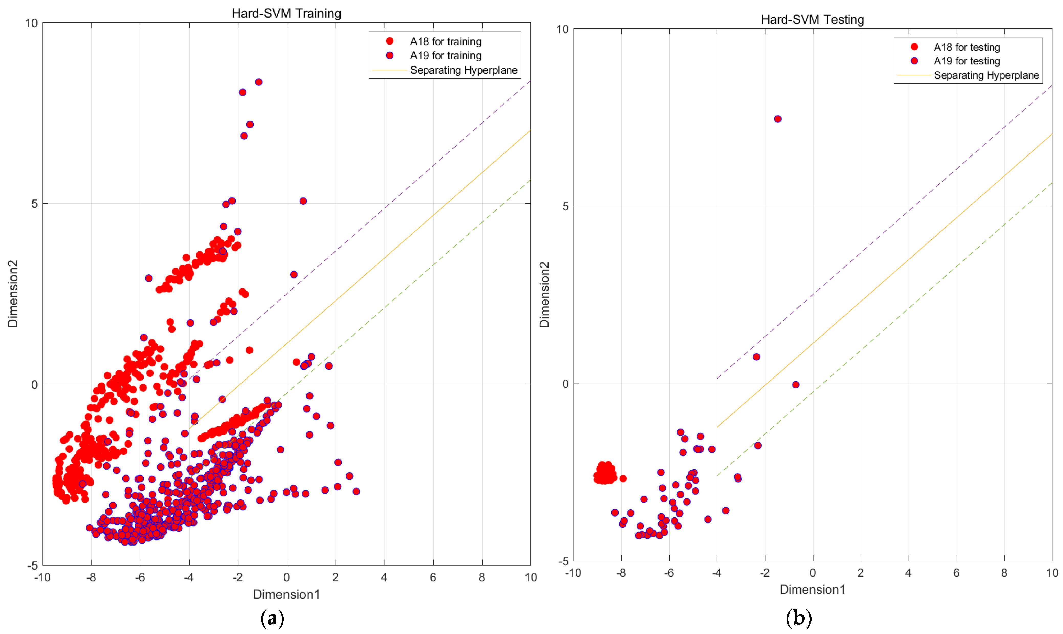
Figure 19.
SVM preliminary segmentation A18 and A19 result graph. (Solid line is the main decision boundary, and dashed line is the margin). (a) SVM model by train set; (b) SVM model by test set.
Figure 19.
SVM preliminary segmentation A18 and A19 result graph. (Solid line is the main decision boundary, and dashed line is the margin). (a) SVM model by train set; (b) SVM model by test set.
Figure 20.
Confusion matrix diagram for the two-layer classifier model XR-KS. (a) Test set confusion matrix obtained after correction; (b) test set confusion matrix obtained after correction (%).
Figure 20.
Confusion matrix diagram for the two-layer classifier model XR-KS. (a) Test set confusion matrix obtained after correction; (b) test set confusion matrix obtained after correction (%).
Figure 21.
Cross-validation and k = 5 results. (a) First-split training set confusion matrix; (b) first-split testing set confusion matrix; (c) second-split training set confusion matrix; (d) second-split testing set confusion matrix; (e) third-split training set confusion matrix; (f) third-split testing set confusion matrix; (g) fourth-split training set confusion matrix; (h) fourth-split testing set confusion matrix; (i) fifth-split training set confusion matrix; (j) fifth-split testing set confusion matrix.
Figure 22.
UCI DSA of the SVM model ROC curve and AUC value by train:test = 9:1. (a) ROC curves and AUC values of SVM confounded A9, A13 and A18, A19 class result plots; (b) ROC curves and AUC values of SVM confounded A9 and A13 class result plots; (c) ROC curves and AUC values of SVM confounded A18 and A19 class result plots.
Table 1.
Comparison between datasets: UCI DSA, UCI HAR, WISDM, and UCI ADL.
Table 1.
Comparison between datasets: UCI DSA, UCI HAR, WISDM, and UCI ADL.
| | UCI DSA | UCI HAR | WISDM | IM-WSHA |
|---|
| Type of activity studied | Short-time | Short-time | Short-time | Short-time |
| Different volunteers | Yes | Yes | Yes | Yes |
| Volunteer numbers | 4 | 30 | 36 | 10 |
| Fixed sensor frequency | Yes | Yes | Yes | Yes |
| Instances | 1,140,000 | 10,299 | 1,098,207 | 125,955 |
| Sensors | Acc. and gyro. | Acc. and gyro. | Acc | Acc. and gyro. |
| Sensor data collection | Comprehensively | Comprehensively | Selectively | Selectively |
| Sensor type | Phone | Phone | Phone | IMU |
| Sensor number | 3 | 3 | 1 | 3 |
| Activities type | 19 | 6 | 6 | 11 |
Table 2.
Table of specific actions and corresponding codes in the text.
Table 2.
Table of specific actions and corresponding codes in the text.
| Behavior | Codes | Behavior | Codes |
|---|
| Sitting | A1 | walking on a treadmill with a speed of 4 km/h (15 deg inclined positions) | A11 |
| Standing | A2 | running on a treadmill with a speed of 8 km/h | A12 |
| Lying on back | A3 | exercising on a stepper | A13 |
| Lying on right side | A4 | exercising on a cross trainer | A14 |
| Ascending stairs | A5 | cycling on an exercise bike in horizontal | A15 |
| Descending stairs | A6 | cycling on an exercise bike in vertical positions | A16 |
| Standing in an elevator still | A7 | rowing | A17 |
| Moving around in an elevator | A8 | jumping | A18 |
| Walking in a parking lot | A9 | playing basketball | A19 |
| Walking on a treadmill with a speed of 4 km/h (in flat) | A10 | | |
Table 3.
Number of features and error rate, accuracy rate, training times, and running time (mean ± std).
Table 3.
Number of features and error rate, accuracy rate, training times, and running time (mean ± std).
| Number of Features | Error Rate | Accuracy Rate | Training Time (s) | Running Time (s) |
|---|
| 1 | 81.5438 (±1.13)% | 18.4561 (±1.13)% | 251.53 (±7.292) | 8.1802 (±0.165) |
| 6 | 22.1995 (±1.24)% | 77.8004 (±1.24)% | 238.55 (±4.063) | 4.9149 (±0.08) |
| 21 | 11.1931 (±1.49)% | 88.8068 (±1.49)% | 203.36 (±4.209) | 4.5172 (±0.78) |
| 31 | 10.7098 (±1.62)% | 89.2901 (±1.62)% | 202.83 (±0.151) | 4.4230 (±0.73) |
| 41 | 10.6396 (±1.79)% | 89.3603 (±1.79)% | 217.82 (±2.107) | 4.8204 (±0.68) |
| 45 | 10.4229 (±1.86)% | 89.5770 (±1.86)% | 217.89 (±0.278) | 4.7276 (±0.89) |
Table 4.
Number of decisions and error rate, accuracy rate, training times, and running time (mean ± std).
Table 4.
Number of decisions and error rate, accuracy rate, training times, and running time (mean ± std).
| Number of Decisions Tree | Error Rate | Accuracy Rate | Training Time (s) | Running Time (s) |
|---|
| 1 | 15.0119 (±1.12)% | 84.9881 (±1.12)% | 13.3845 (±1.507) | 0.2793 (±0.126) |
| 6 | 11.7283 (±1.25)% | 88.2717 (±1.25)% | 32.5361 (±0.580) | 0.7068 (±0.062) |
| 11 | 11.3098 (±1.39)% | 88.6902 (±1.39)% | 53.4840 (±0.665) | 1.1963 (±0.019) |
| 21 | 11.0589 (±1.51)% | 88.9411 (±1.51)% | 95.7831 (±0.345) | 2.2481 (±0.059) |
| 31 | 10.8791 (±1.46)% | 89.1209 (±1.46)% | 141.0272 (±4.273) | 3.2747 (±0.017) |
| 41 | 10.7501 (±1.81)% | 89.2499 (±1.81)% | 187.3081 (±10.173) | 4.4448 (±0.106) |
| 50 | 10.5211 (±1.95)% | 89.4789 (±1.95)% | 215.6206 (±20.992) | 5.0635 (±1.308) |
Table 5.
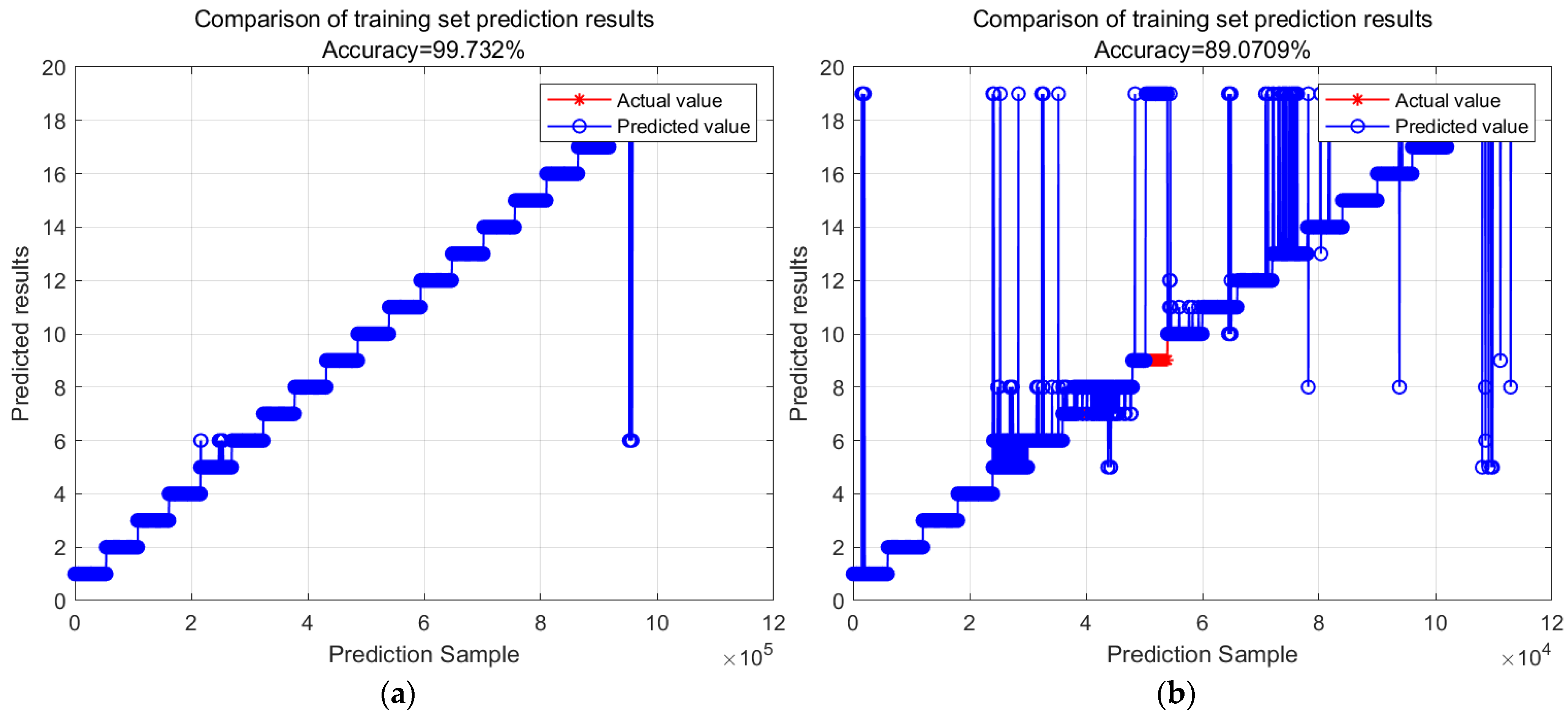
Random forest model based on XGBoost feature selection algorithm result table of UCI DSA (mean ± std). (The experiments were set up with different ratios of test and validation sets and repeated five times).
Table 5.
Random forest model based on XGBoost feature selection algorithm result table of UCI DSA (mean ± std). (The experiments were set up with different ratios of test and validation sets and repeated five times).
| Ratio (Training: Testing) | UCI DSA Accuracy Rate and Time |
|---|
| Training Data | Testing Data | Running Time (s) |
|---|
| 9:1 | 99.7322 (±0.08)% | 89.0709 (±1.59)% | 5.124 (±0.29) |
| 8:2 | 99.5669 (±0.12)% | 85.1812 (±1.63)% | 5.243 (±0.28) |
| 7:3 | 99.3541 (±0.13)% | 79.3321 (±1.76)% | 5.165 (±0.36) |
| 6:4 | 99.2145 (±0.15)% | 74.0732 (±1.86)% | 5.146 (±0.15) |
| 5:5 | 99.6656 (±0.17)% | 69.5766 (±2.12)% | 5.234 (±0.34) |
| 4:6 | 99.6706 (±0.21)% | 68.6753 (±2.65)% | 5.091 (±0.39) |
Table 6.
Random forest model based on the XGBoost feature selection algorithm result table between datasets: UCI DSA, UCI HAR, WISDM, and UCI ADL (mean ± std) (the experimental setup is like the one in
Table 5).
Table 6.
Random forest model based on the XGBoost feature selection algorithm result table between datasets: UCI DSA, UCI HAR, WISDM, and UCI ADL (mean ± std) (the experimental setup is like the one in
Table 5).
Ratio (Training:
Testing) | UCI HAR Accuracy Rate and Time | WISDM Accuracy Rate and Time | IM-WSHA Accuracy Rate and Time |
|---|
| Training Data | Testing Data | Running Time (s) | Training Data | Testing Data | Running Time (s) | Training Data | Testing Data | Running Time (s) |
|---|
| 9:1 | 100 (±0.01)% | 92.7863 (±1.01)% | 0.38951 (±0.01) | 99.9999 (±0.54)% | 92.5161 (±0.58)% | 27.7856 (±1.12) | 99.9974 (±0.05)% | 84.1109 (±1.07)% | 4.2978 (±0.51) |
| 8:2 | 100 (±0.01)% | 90.9886 (±1.13)% | 0.38611 (±0.02) | 99.9018 (±0.76)% | 92.4081 (±0.69)% | 27.6143 (±1.16) | 99.6043 (±0.13)% | 81.4639 (±1.13)% | 4.3386 (±0.55) |
| 7:3 | 100 (±0.01)% | 91.5774 (±1.22)% | 0.38302 (±0.04) | 99.8996 (±0.81)% | 91.9205 (±0.91)% | 27.5283 (±1.08) | 99.6632 (±0.14)% | 76.5923 (±1.24)% | 4.2999 (±0.55) |
| 6:4 | 100 (±0.01)% | 90.6069 (±1.34)% | 0.39912 (±0.02) | 99.9007 (±0.96)% | 91.7434 (±1.21)% | 27.1654 (±1.16) | 99.6756 (±0.12)% | 71.1226 (±1.45)% | 4.2382 (±0.61) |
| 5:5 | 100 (±0.01)% | 90.9319 (±1.62)% | 0.39054 (±0.03) | 99.6061 (±1.15)% | 91.7573 (±1.36)% | 26.5401 (±1.19) | 99.6656 (±0.11)% | 68.6637 (±1.32)% | 3.9513 (±0.62) |
| 4:6 | 100 (±0.01)% | 88.6398 (±1.72)% | 0.37715 (±0.01) | 99.9014 (±1.53)% | 90.9253 (±1.49)% | 25.2154 (±1.18) | 99.6706 (±0.18)% | 65.8418 (±1.23)% | 3.9411 (±0.36) |
Table 7.
Confusing action classification table.
Table 7.
Confusing action classification table.
| Confussing Category | Easily Confused Actions |
|---|
| Confusing category I | A9, A13, A18, A19 |
| Confusing category II | A5, A6 |
| Confusing category III | A7, A8 |
Table 8.
Random forest result (mean ± std) table between datasets: UCI DSA, UCI HAR, WISDM, and UCI ADL.
Table 8.
Random forest result (mean ± std) table between datasets: UCI DSA, UCI HAR, WISDM, and UCI ADL.
Ratio (Training:
Testing) | A9, A13 and A18,A19 Accuracy Rate and Running Time | A9 and A13 Accuracy Rate and Running Time | A18 and A19 Accuracy Rate and Running Time |
|---|
| Training Data | Testing Data | Running Time (s) | Training Data | Testing Data | Running Time (s) | Training Data | Testing Data | Running Time (s) |
|---|
| 9:1 | 97.9444 (±0.13)% | 95.0 (±0.16)% | 0.9401 (±0.15) | 84.0 (±0.15)% | 59.0 (±0.16)% | 0.1802 (±0.071) | 86.4444 (±0.14)% | 92.0 (±0.16)% | 0.1605 (±0.017) |
| 8:2 | 98.0 (±0.11)% | 96.2512 (±0.13)% | 0.8749 (±0.13) | 79.8714 (±0.19)% | 70.0 (±0.19)% | 0.1524 (±0.045) | 84.8751 (±0.18)% | 95.50 (±0.14)% | 0.1413 (±0.065) |
| 7:3 | 98.0 (±0.15)% | 97.0 (±0.15)% | 0.4801 (±0.14) | 76.0 (±0.16)% | 79.6667 (±0.13)% | 0.0953 (±0.065) | 83.7143 (±0.16)% | 94.6667 (±0.16)% | 0.09714 (±0.094) |
| 6:4 | 97.8333 (±0.14)% | 97.75 (±0.14)% | 0.4146 (±0.16) | 73.0 (±0.16)% | 85.0 (±0.12)% | 0.07241 (±0.014) | 83.8333 (±0.16)% | 92.0 (±0.17)% | 0.07048 (±0.053) |
| 5:5 | 99.90 (±0.14)% | 96.95 (±0.17)% | 0.4521 (±0.091) | 65.80 (±0.14)% | 87.60 (±0.11)% | 0.05512 (±0.069) | 93.40 (±0.16)% | 83.40 (±0.17)% | 0.05041 (±0.047) |
| 4:6 | 99.91 (±0.14)% | 97.41 (±0.14)% | 0.2413 (±0.075) | 84.75 (±0.14)% | 85.0 (±0.17)% | 0.03338 (±0.064) | 92.75 (±0.19)% | 85.3333 (±0.16)% | 0.02581 (±0.034) |
Table 9.
Comparison of recognition accuracy of the proposed method with other state-of-the-art methods over UCI DSA, UCI HAR, WISDM, and IM-WSHA datasets (Bolding in the table indicates the methodology of this paper)..
Table 9.
Comparison of recognition accuracy of the proposed method with other state-of-the-art methods over UCI DSA, UCI HAR, WISDM, and IM-WSHA datasets (Bolding in the table indicates the methodology of this paper)..
| Reference Study | Model | UCI DSA | UCI HAR | WISDM | IM-WSHA |
|---|
| Qiu et al. (2016) [37] | Estimation algorithm [38] | | | | 80.49% |
| Gochoo et al. (2021) [38] | RPLB [39] | | | | 83.18% |
| Halim et al. (2022) [39] | hybrid descriptors and random forest [40] | | | | 91.45% |
| Ghadi et al. (2022) [40] | MS-DLD [41] | | | | 95.0% |
| Koşar et al. (2023) [41] | Deep CNN-LSTM [42] | | 93.11% | | |
| Kobayashi et al. (2023) [42] | MarNASNet [43] | | 94.50% | 88.92% | |
| Wang et al. (2023) [43] | DMEFAM [44] | | 96% | 97.9% | |
| Dua, N et al. (2023) [44] | Deep CNN-GRU [45] | | 96.20% | 97.21% | |
| Imran et al. (2023) [45] | EdgeHARNet [46] | | | 94.036% | |
| Zhang et al. (2023) [46] | BLSTM [47] | | 98.37% | 99.01% | |
| Thakur et al. (2023) [47] | CAEL-HAR [48] | | 96.45% | 98.57% | |
| Li et al. (2016) [48] | MVTS [49] | 91.35% | | | |
| Present paper | XR-KS | 97.69% | 97.92% | 98.12% | 90.6% |
Table 10.
Mean (±std) k = 5 and cross-validation XR model results of UCI DSA. (Five repetitions of the experiment were conducted to obtain the mean and confidence intervals).
Table 10.
Mean (±std) k = 5 and cross-validation XR model results of UCI DSA. (Five repetitions of the experiment were conducted to obtain the mean and confidence intervals).
| K | Training Data Accuracy | Testing Data Accuracy | Training
Running Time (s) | Test
Running Time (s) |
|---|
| 1 | 99.7414% (±0.91) | 99.1421% (±0.94) | 463.0862 (±8.53) | 51.0272 (±1.81) |
| 2 | 99.8561% (±0.84) | 99.1421% (±0.45) | 408.6202 (±8.45) | 48.6971 (±2.31) |
| 3 | 99.7651% (±0.57) | 99.1421% (±0.41) | 370.8408 (±9.54) | 42.7105 (±2.45) |
| 4 | 99.8234% (±0.61) | 99.1421% (±0.61) | 377.3214 (±7.14) | 40.2905 (±2.16) |
| 5 | 99.8317% (±0.74) | 99.1421% (±0.37) | 386.5293 (±7.41) | 39.6749 (±1.97) |
Table 11.
KS model AUC mean (±std) results of UCI DSA. (Five repetitions of the experiment were conducted to obtain the mean and confidence intervals).
Table 11.
KS model AUC mean (±std) results of UCI DSA. (Five repetitions of the experiment were conducted to obtain the mean and confidence intervals).
| Ratio (Training: Testing) | A9, A13 and A18, A19 AUC | A9, A13 AUC | A18, A19 AUC |
|---|
| 9:1 | 0.98491 (±0.01) | 0.77412 (±0.01) | 0.97961 (±0.02) |
| 8:2 | 0.99155 (±0.01) | 0.90591 (±0.01) | 0.97573 (±0.01) |
| 7:3 | 0.99229 (±0.01) | 0.95818 (±0.01) | 0.97361 (±0.04) |
| 6:4 | 0.99386 (±0.03) | 0.97513 (±0.01) | 0.96473 (±0.03) |
| 5:5 | 0.99153 (±0.01) | 0.98271 (±0.02) | 0.86586 (±0.01) |
| 4:6 | 0.99324 (±0.01) | 0.93727 (±0.03) | 0.87724 (±0.01) |


