
CORTO: The Celestial Object Rendering TOol at DART Lab

Abstract
:1. Introduction
- PANGU [7,8,9] stands for Planetary Planet and Asteroid Natural scene Generation Utility and is considered the state of the art in rendering celestial bodies. It is a tool with robust, long-lasting, and documented development designed by the University of Dundee for the ESA. PANGU supports various advanced functionalities and is extensively used as the industry standard for ESA projects involving visual-based navigation algorithms. However, access to the software is regulated via licenses and often requires direct involvement with an ESA project as a pre-requisite.
- SurRender (v.6.0) [10,11] is proprietary software by Airbus Defense and Space (https://www.airbus.com/en/products-services/space/customer-services/surrendersoftware, accessed on 8 August 2023) that has been successfully used in designing and validating various vision-based applications for space missions in which the company is involved. The software can handle objects such as planets, asteroids, stars, satellites, and spacecraft. It provides detailed models of sensors (cameras, LiDAR) with validated radiometric and geometric models (global or rolling shutter, pupil size, gains, variable point spread functions, noises, etc.). The renderings are based on real-time image generation in OpenGL or raytracing for real-time testing of onboard software. Surface properties are tailored with user-specified reflectance models (BRDF), textures, and normal maps. The addition of procedural details such as fractal albedos, multi-scale elevation structures, 3D models, and distributions of craters and boulders are also supported.
- SISPO [12] stands for Space Imaging Simulator for Proximity Operations and is an open-access image generation tool developed by a group of researchers from the universities of Tartu and Aalto, specifically designed to support a proposed multi-asteroid tour mission [13] and the ESA’s Comet Interceptor mission [14]. SISPO can obtain photo-realistic images of minor bodies and planetary surfaces using Blender (https://www.blender.org/, accessed on 8 August 2023) Cycles and OpenGL (https://www.opengl.org/, accessed on 8 August 2023) as rendering engines. Additionally, advanced scattering functions written in Open Shading Language (OSL) are made available (https://bitbucket.org/mariofpalos/asteroid-image-generator/wiki/Home, accessed on 26 of October 2023) that can be used in the shading tab in Blender to model surface reflectance, greatly enhancing the output quality.
- Vizard (https://hanspeterschaub.info/basilisk/Vizard/Vizard.html#, accessed on 15 November 2023) is a Unity-based visualization tool capable of displaying the simulation output of the Basilisk (v.2.2.0) [15] software (https://hanspeterschaub.info/basilisk/, accessed on 15 of November 2023). Its main purpose is to visualize the state of the spacecraft; however, it has also been used for optical navigation assessment around Mars [16,17,18] and can simulate both terrestrial and small body scenarios [19].
- The simulation tools illustrated in [20,21] implement high-fidelity regolith-specific reflectance models using Blender and Unreal Engine 5 (https://www.unrealengine.com/en-US, accessed on 8 August 2023). The tools can render high-fidelity imagery for close proximity applications, particularly about small bodies, focusing on the high-fidelity simulation of boulder fields over their surfaces.
- AstroSym [22], developed in Python, provides a source of images for closed-loop simulation for Guidance Navigation and Control (GNC) systems for landing and close-proximity operations around asteroids.
- SPyRender [23], also developed in Python, is used to generate high-fidelity images of the comet 67P for training data-driven IP methods for navigation applications.
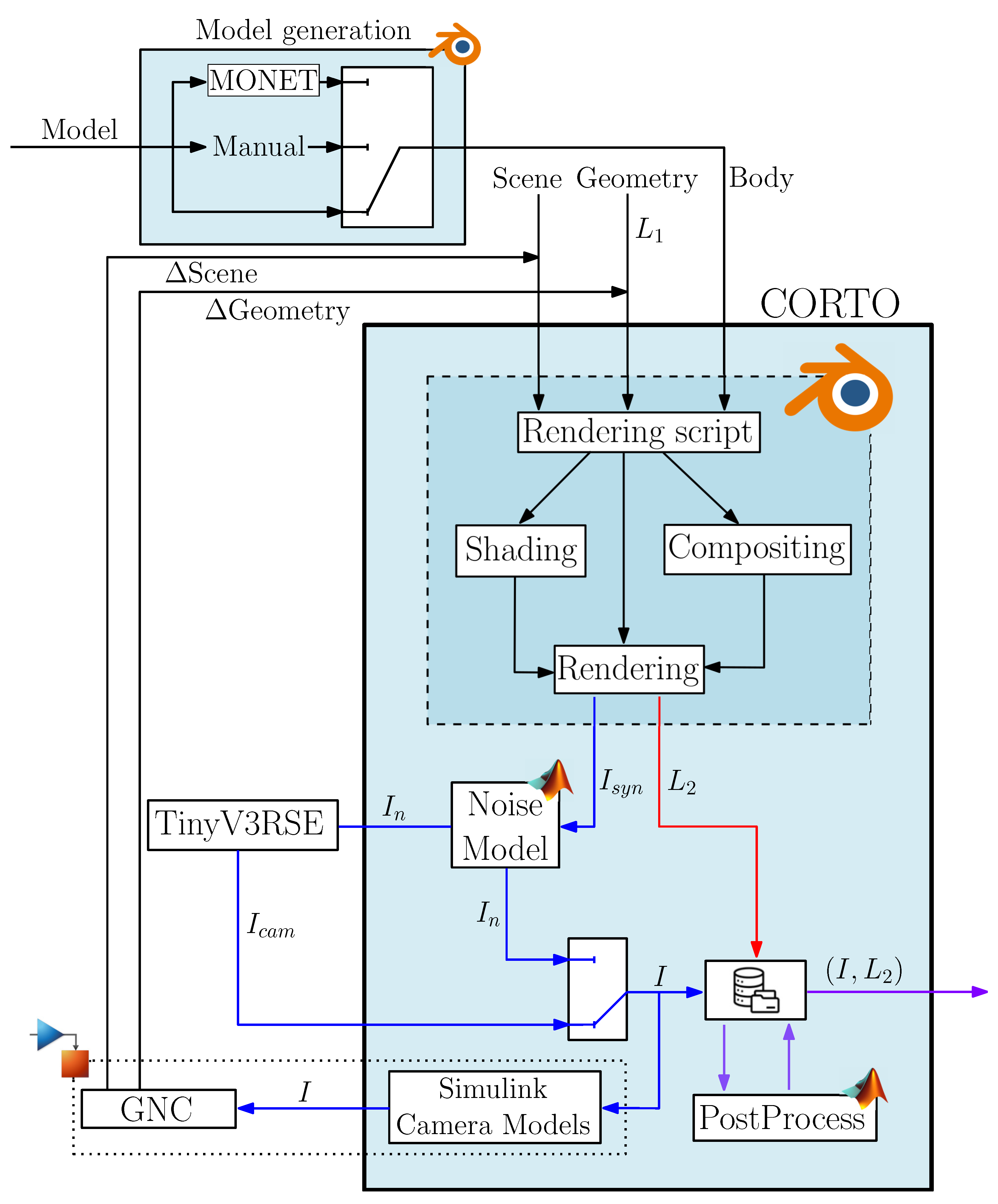
2. Architecture of the Tool
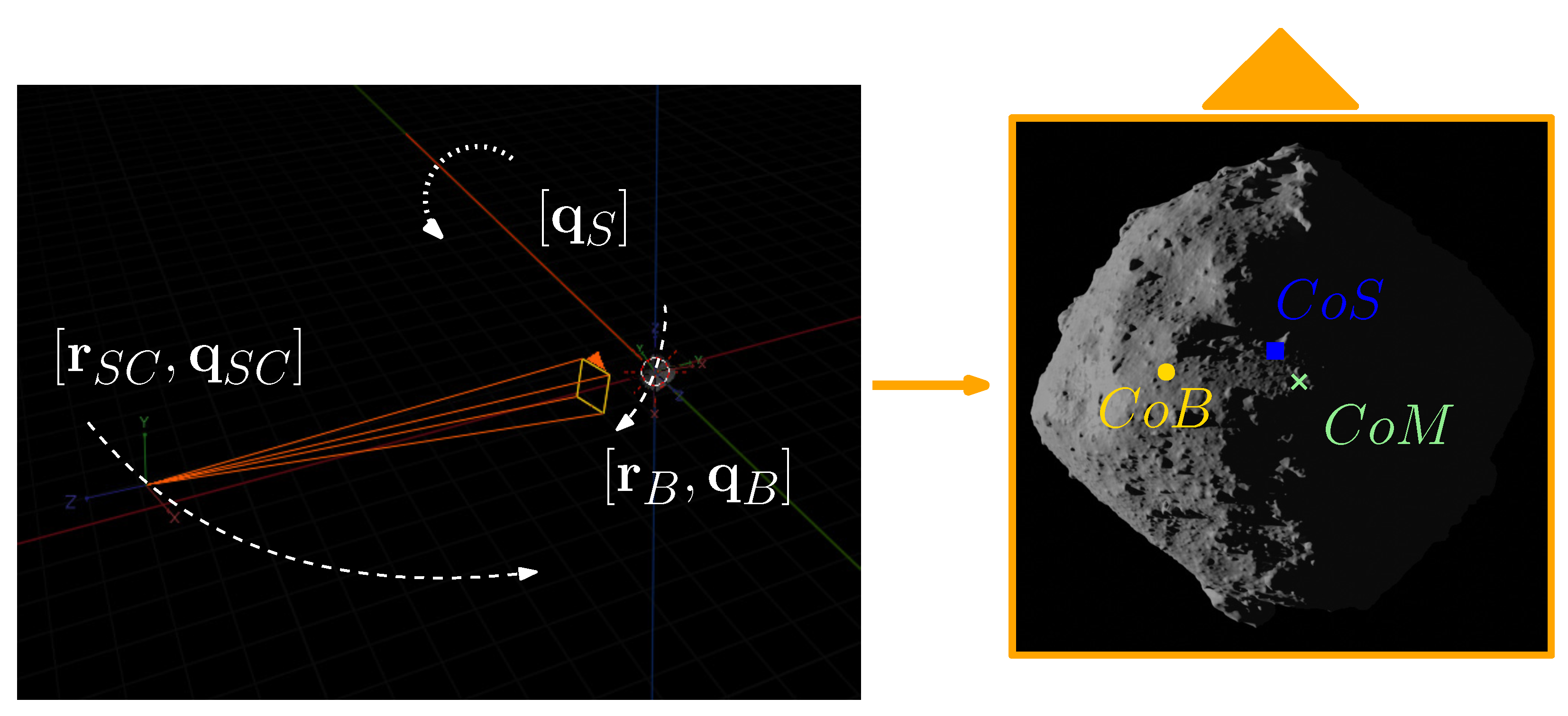
2.1. Object Handling
2.2. Rendering
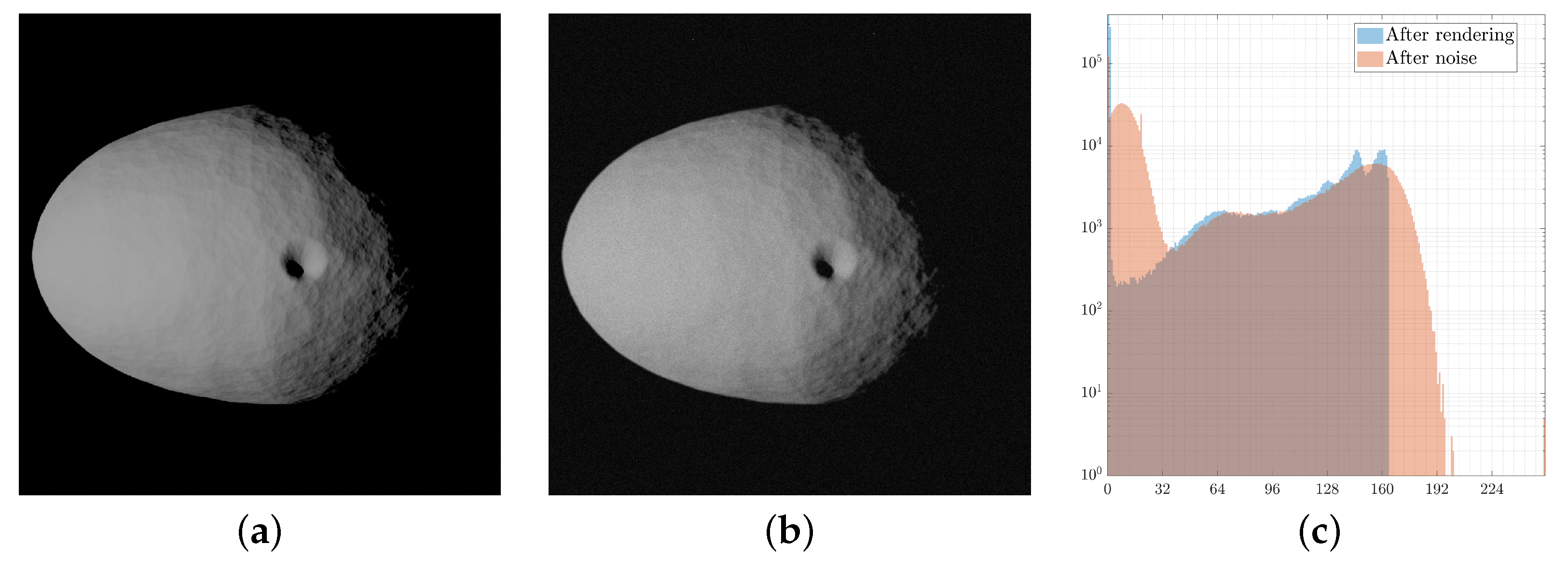
2.3. Noise Modelling
2.4. Hardware-in-the-Loop
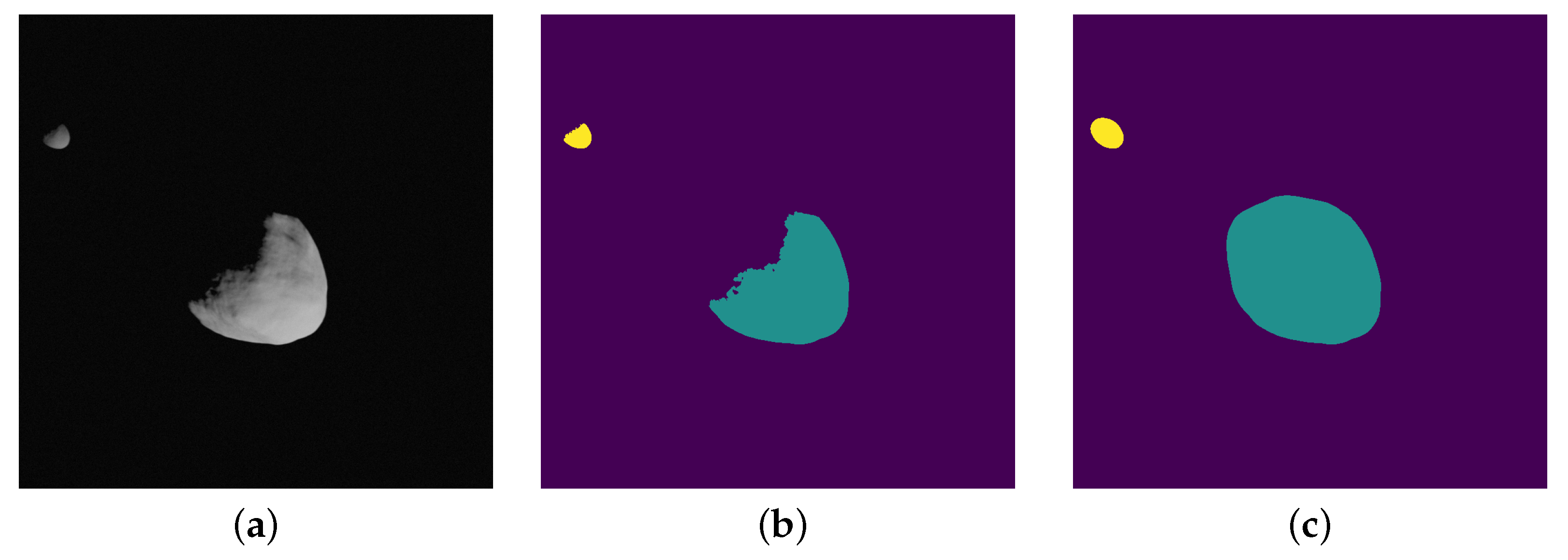
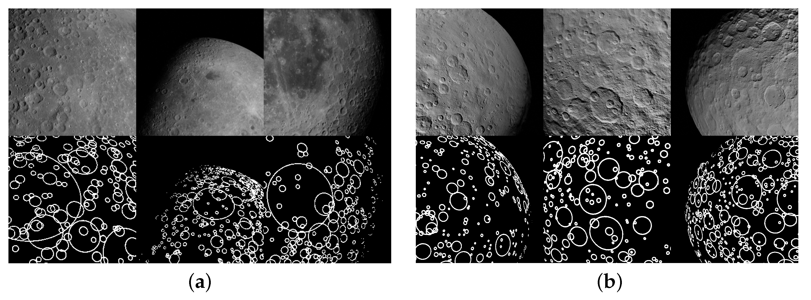
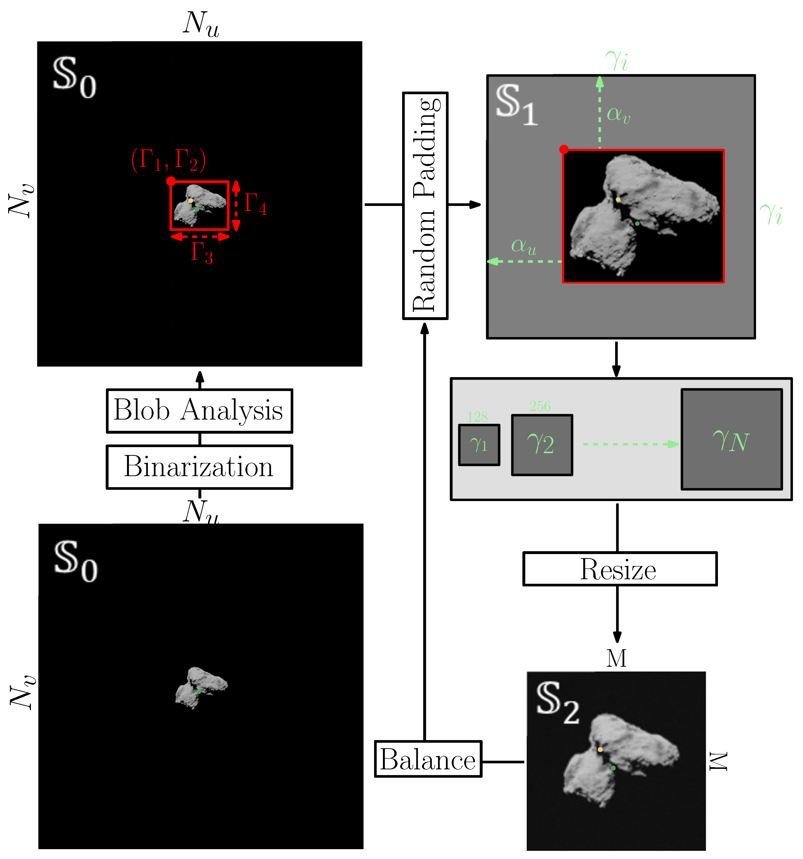
2.5. Post-Processing
2.6. Reproduce Previously Flown Missions
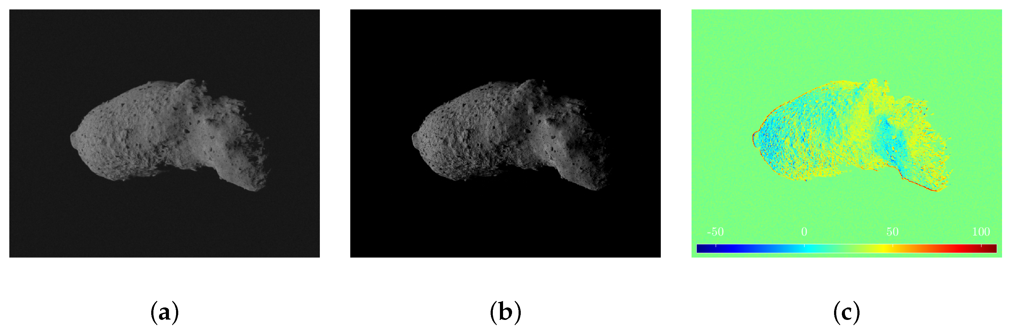
3. Validation
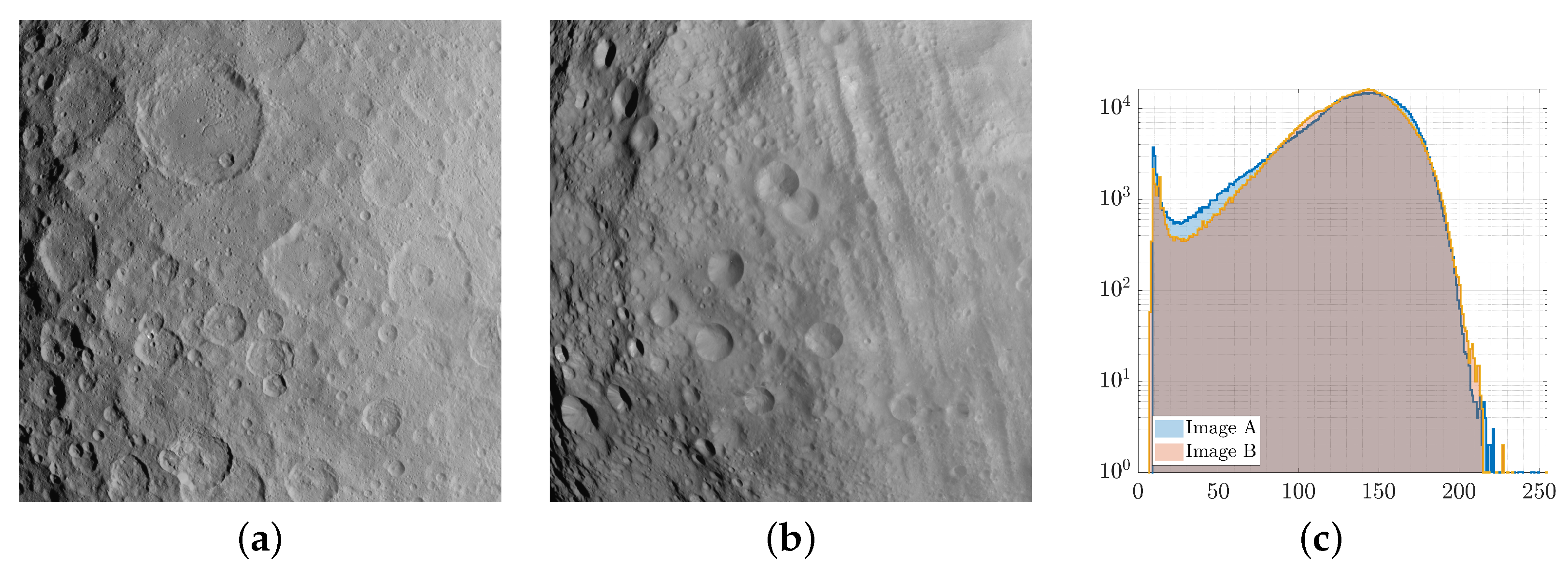
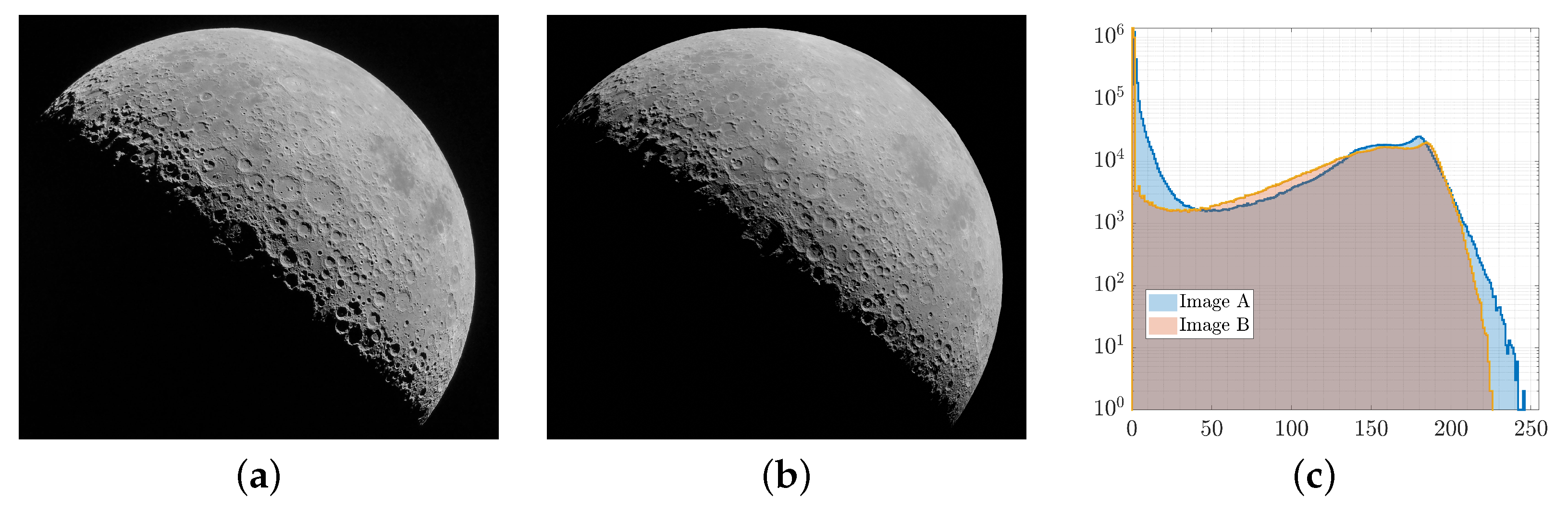
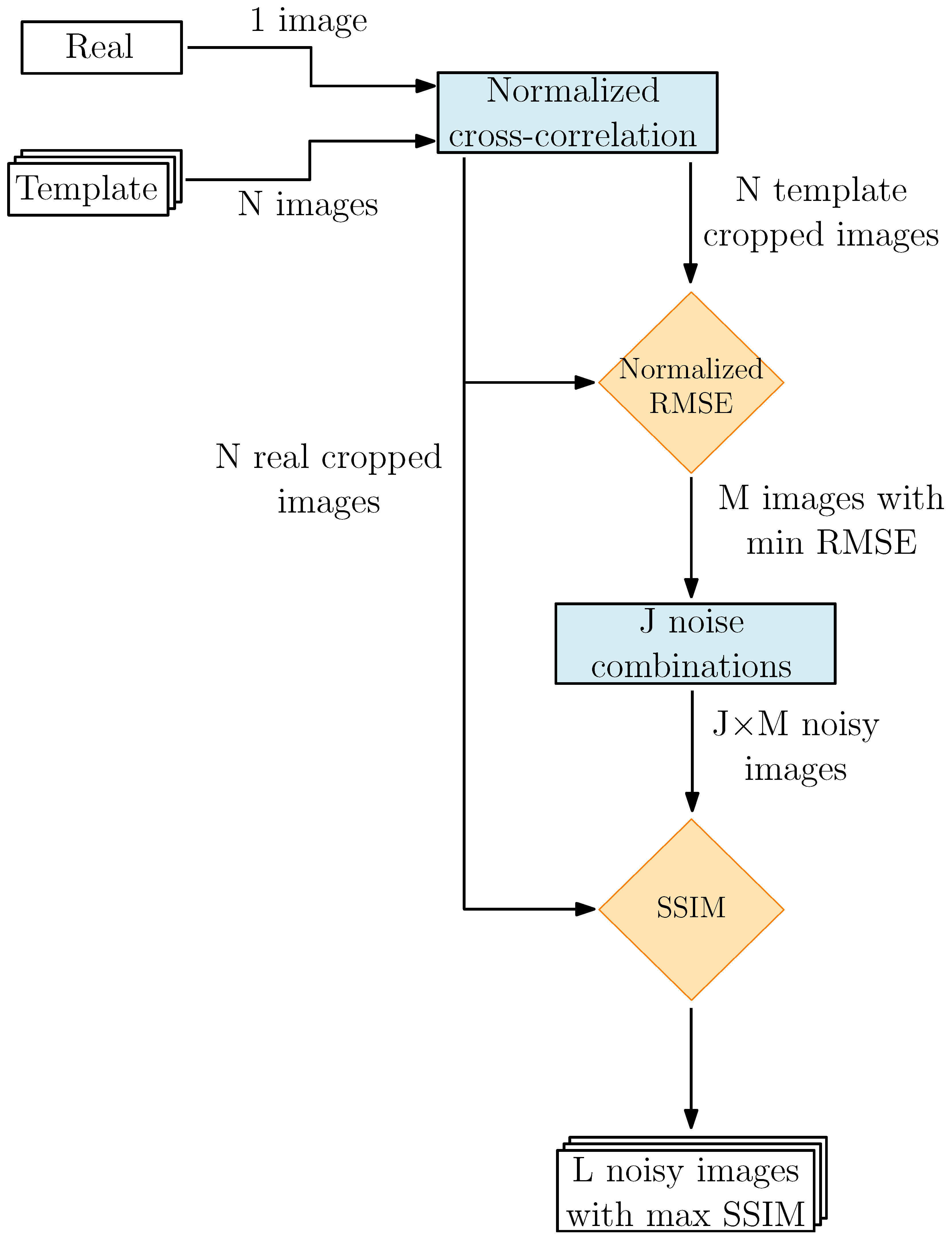
3.1. The Validation Pipeline
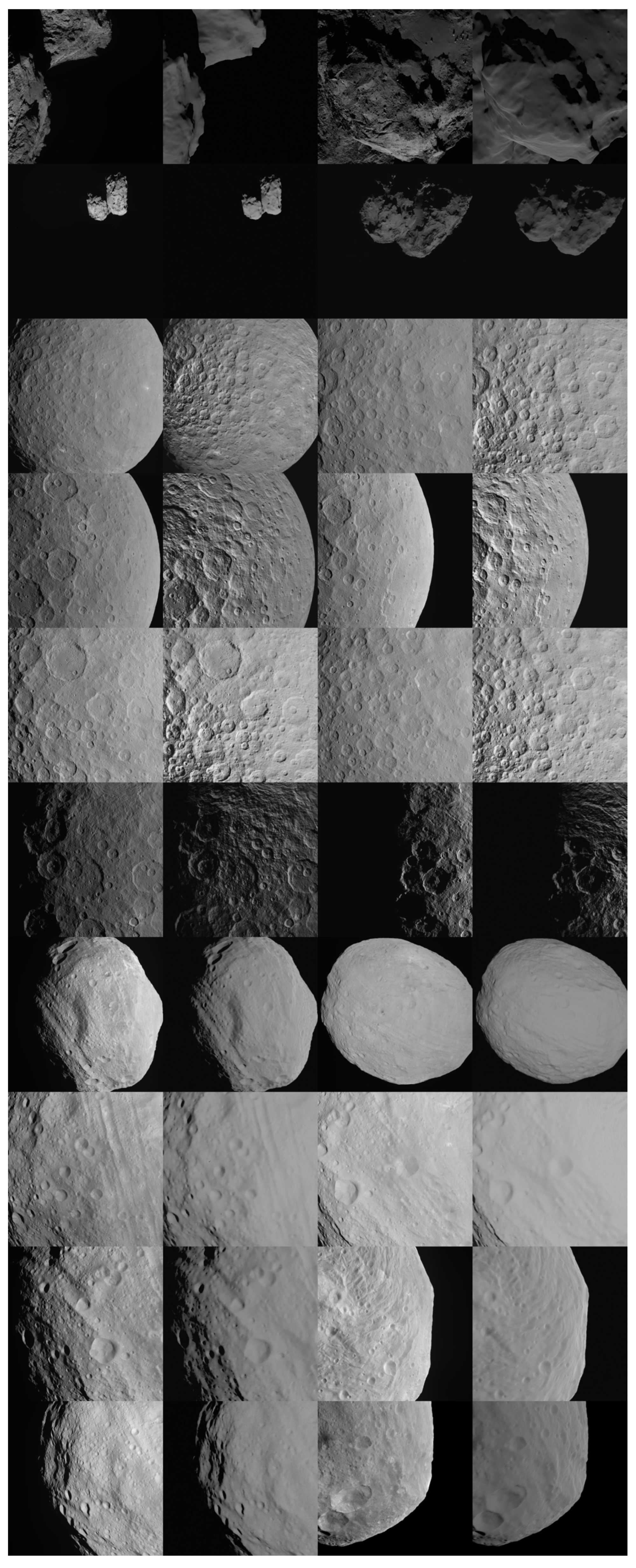
3.2. Validation Examples
4. Case Studies
5. Conclusions and Future Implementations
Author Contributions
Funding
Institutional Review Board Statement
Informed Consent Statement
Data Availability Statement
Conflicts of Interest
Abbreviations
| CORTO | Celestial Object Rendering TOol |
| DART | Deep-Space Astrodynamic Research and Technology |
| GNC | Guidance Navigation and Control |
| HIL | Hardware-In-the-Loop |
| IP | Image Processing |
| MONET | Minor bOdy GeNErator Tool |
| NRMSE | Normalized Root Mean Square Error |
| OSL | Open Shading Language |
| PBSDF | Principled Bi-directional Scatter Distribution Function |
| SSIM | Structural Similarity Index Measure |
| TinyV3RSE | Tiny Versatile 3D Reality Simulation Environment |
Appendix A
References
- Prockter, L.; Murchie, S.; Cheng, A.; Krimigis, S.; Farquhar, R.; Santo, A.; Trombka, J. The NEAR shoemaker mission to asteroid 433 eros. Acta Astronaut. 2002, 51, 491–500. [Google Scholar] [CrossRef]
- Yoshikawa, M.; Kawaguchi, J.; Fujiwara, A.; Tsuchiyama, A. Hayabusa sample return mission. Asteroids IV 2015, 1, 1. [Google Scholar]
- Glassmeier, K.H.; Boehnhardt, H.; Koschny, D.; Kührt, E.; Richter, I. The Rosetta mission: Flying towards the origin of the solar system. Space Sci. Rev. 2007, 128, 1–21. [Google Scholar] [CrossRef]
- Russell, C.T.; Raymond, C.A. The Dawn Mission to Vesta and Ceres. In The Dawn Mission to Minor Planets 4 Vesta and 1 Ceres; Russell, C., Raymond, C., Eds.; Springer: New York, NY, USA, 2012; pp. 3–23. [Google Scholar] [CrossRef]
- Watanabe, S.i.; Tsuda, Y.; Yoshikawa, M.; Tanaka, S.; Saiki, T.; Nakazawa, S. Hayabusa2 mission overview. Space Sci. Rev. 2017, 208, 3–16. [Google Scholar] [CrossRef]
- Lauretta, D.; Balram-Knutson, S.; Beshore, E.; Boynton, W.; Drouet d’Aubigny, C.; DellaGiustina, D.; Enos, H.; Golish, D.; Hergenrother, C.; Howell, E.; et al. OSIRIS-REx: Sample return from asteroid (101955) Bennu. Space Sci. Rev. 2017, 212, 925–984. [Google Scholar] [CrossRef]
- Martin, I.; Dunstan, M.; Gestido, M.S. Planetary surface image generation for testing future space missions with pangu. In Proceedings of the 2nd RPI Space Imaging Workshop, Saratoga Springs, NY, USA, 28–30 October 2019; pp. 1–13. [Google Scholar]
- Martin, I.; Dunstan, M. PANGU v6: Planet and Asteroid Natural Scene Generation Utility; University of Dundee: Dundee, UK, 2021. [Google Scholar]
- Parkes, S.; Martin, I.; Dunstan, M.; Matthews, D. Planet surface simulation with pangu. In Proceedings of the Space OPS 2004 Conference, Montreal, QC, Canada, 17–21 May 2004; p. 389. [Google Scholar]
- Lebreton, J.; Brochard, R.; Baudry, M.; Jonniaux, G.; Salah, A.H.; Kanani, K.; Goff, M.L.; Masson, A.; Ollagnier, N.; Panicucci, P.; et al. Image simulation for space applications with the SurRender software. In Proceedings of the 11th International ESA Conference on Guidance, Navigation & Control Systems, Online, 22–25 June 2021; pp. 1–16. [Google Scholar]
- Brochard, R.; Lebreton, J.; Robin, C.; Kanani, K.; Jonniaux, G.; Masson, A.; Despré, N.; Berjaoui, A. Scientific image rendering for space scenes with the SurRender software. arXiv 2018, arXiv:1810.01423. [Google Scholar]
- Pajusalu, M.; Iakubivskyi, I.; Schwarzkopf, G.J.; Knuuttila, O.; Väisänen, T.; Bührer, M.; Palos, M.F.; Teras, H.; Le Bonhomme, G.; Praks, J.; et al. SISPO: Space Imaging Simulator for Proximity Operations. PLoS ONE 2022, 17, e0263882. [Google Scholar] [CrossRef]
- Iakubivskyi, I.; Mačiulis, L.; Janhunen, P.; Dalbins, J.; Noorma, M.; Slavinskis, A. Aspects of nanospacecraft design for main-belt sailing voyage. Adv. Space Res. 2021, 67, 2957–2980. [Google Scholar] [CrossRef]
- Snodgrass, C.; Jones, G.H. The European Space Agency’s Comet Interceptor lies in wait. Nat. Commun. 2019, 10. [Google Scholar] [CrossRef]
- Kenneally, P.W.; Piggott, S.; Schaub, H. Basilisk: A Flexible, Scalable and Modular Astrodynamics Simulation Framework. J. Aerosp. Inf. Syst. 2020, 17, 496–507. [Google Scholar] [CrossRef]
- Teil, T.F. Optical Navigation using Near Celestial Bodies for Spacecraft Autonomy. Ph.D. Thesis, University of Colorado, Boulder, CO, USA, 2020. [Google Scholar]
- Teil, T.; Schaub, H.; Kubitschek, D. Centroid and Apparent Diameter Optical Navigation on Mars Orbit. J. Spacecr. Rocket. 2021, 58, 1107–1119. [Google Scholar] [CrossRef]
- Teil, T.; Bateman, S.; Schaub, H. Autonomous On-orbit Optical Navigation Techniques For Robust Pose-Estimation. Adv. Astronaut. Sci. Aas Guid. Navig. Control. 2020, 172. [Google Scholar]
- Teil, T.; Bateman, S.; Schaub, H. Closed-Loop Software Architecture for Spacecraft Optical Navigation and Control Development. J. Astronaut. Sci. 2020, 67, 1575–1599. [Google Scholar] [CrossRef]
- Villa, J.; Bandyopadhyay, S.; Morrell, B.; Hockman, B.; Bhaskaran, S.; Nesnas, I. Optical navigation for autonomous approach of small unknown bodies. In Proceedings of the 43rd Annual AAS Guidance, Navigation & Control Conference, Maui, HI, USA, 13–17 January 2019; Volume 30, pp. 1–3. [Google Scholar]
- Villa, J.; Mcmahon, J.; Nesnas, I. Image Rendering and Terrain Generation of Planetary Surfaces Using Source-Available Tools. In Proceedings of the 46th Annual AAS Guidance, Navigation & Control Conference, Breckenridge, CO, USA, 3 February 2023; pp. 1–24. [Google Scholar]
- Peñarroya, P.; Centuori, S.; Hermosín, P. AstroSim: A GNC simulation tool for small body environments. In Proceedings of the AIAA SCITECH 2022 Forum, San Diego, CA, USA, 3–7 January 2022; p. 2355. [Google Scholar]
- Lopez, A.E.; Ghiglino, P.; Sanjurjo-rivo, M. Churinet-Applying Deep Learning for Minor Bodies Optical Navigation. IEEE Trans. Aerosp. Electron. Syst. 2022, 1–14. [Google Scholar] [CrossRef]
- Panicucci, P.; Topputo, F. The TinyV3RSE Hardware-in-the-Loop Vision-Based Navigation Facility. Sensors 2022, 22, 9333. [Google Scholar] [CrossRef]
- Robbins, S.J. A new global database of lunar impact craters >1–2 km: 1. Crater locations and sizes, comparisons with published databases, and global analysis. J. Geophys. Res. Planets 2019, 124, 871–892. [Google Scholar] [CrossRef]
- Zeilnhofer, M. A Global Analysis of Impact Craters on Ceres. Ph.D. Thesis, Northern Arizona University, Flagstaff, AZ, USA, 2020. [Google Scholar]
- Pugliatti, M.; Maestrini, M. Small-body segmentation based on morphological features with a u-shaped network architecture. J. Spacecr. Rocket. 2022, 59, 1821–1835. [Google Scholar] [CrossRef]
- Pugliatti, M.; Maestrini, M. A multi-scale labeled dataset for boulder segmentation and navigation on small bodies. In Proceedings of the 74th International Astronautical Congress, Baku, Azerbaijan, 2–6 October 2023; pp. 1–8. [Google Scholar]
- Buonagura, C.; Pugliatti, M.; Topputo, F. Procedural minor body generator tool for data-driven optical navigation methods. In Proceedings of the 6th CEAS Specialist Conference on Guidance, Navigation and Control-EuroGNC, Berlin, Germany, 3–5 May 2022; pp. 1–15. [Google Scholar]
- Pugliatti, M.; Topputo, F. Boulders identification on small bodies under varying illumination conditions. arXiv 2022, arXiv:2210.16283. [Google Scholar]
- Golish, D.; DellaGiustina, D.; Li, J.Y.; Clark, B.; Zou, X.D.; Smith, P.; Rizos, J.; Hasselmann, P.; Bennett, C.; Fornasier, S.; et al. Disk-resolved photometric modeling and properties of asteroid (101955) Bennu. Icarus 2021, 357, 113724. [Google Scholar] [CrossRef]
- Seeliger, H. Zur photometrie des saturnringes. Astron. Nachrichten 1884, 109, 305. [Google Scholar] [CrossRef]
- Buratti, B.; Hicks, M.; Nettles, J.; Staid, M.; Pieters, C.; Sunshine, J.; Boardman, J.; Stone, T. A wavelength-dependent visible and infrared spectrophotometric function for the Moon based on ROLO data. J. Geophys. Res. 2011, 116. [Google Scholar] [CrossRef]
- Akimov, L.A. Influence of mesorelief on the brightness distribution over a planetary disk. Sov. Astron. 1975, 19, 385. [Google Scholar]
- Akimov, L.A. On the brightness distributions over the lunar and planetary disks. Astron. Zhurnal 1979, 56, 412. [Google Scholar]
- McEwen, A.S. Photometric functions for photoclinometry and other applications. Icarus 1991, 92, 298–311. [Google Scholar] [CrossRef]
- Minnaert, M. The reciprocity principle in lunar photometry. Astrophys. J. 1941, 93, 403–410. [Google Scholar] [CrossRef]
- Szeliski, R. Computer Vision, 2nd ed.; Springer International Publishing: Cham, Switzerland, 2022. [Google Scholar] [CrossRef]
- Christian, J.A. Optical Navigation for a Spacecraft in a Planetary System. Ph.D. Thesis, University of Texas, Austin, TX, USA, 2010. [Google Scholar]
- Kisantal, M.; Sharma, S.; Park, T.H.; Izzo, D.; Märtens, M.; D’Amico, S. Satellite Pose Estimation Challenge: Dataset, Competition Design, and Results. IEEE Trans. Aerosp. Electron. Syst. 2020, 56, 4083–4098. [Google Scholar] [CrossRef]
- Piccinin, M. Spacecraft Relative Navigation with Electro-Optical Sensors around Uncooperative Targets. Ph.D. Thesis, Politecnico di Milano, Milan, Italy, 2023. [Google Scholar]
- Dunstan, M.; Martin, I. Planet and Asteroid Natural Scene Generation Utility; University of Dundee: Dundee, UK, 2021; pp. 352–355. [Google Scholar]
- Lewis, J.P. Fast normalized cross-correlation. Vision Interface 1995, 95, 120. [Google Scholar]
- Chai, T.; Draxler, R.R. Root mean square error (RMSE) or mean absolute error (MAE)?–Arguments against avoiding RMSE in the literature. Geosci. Model Dev. 2014, 7, 1247–1250. [Google Scholar] [CrossRef]
- Wang, Z.; Bovik, A.; Sheikh, H.; Simoncelli, E. Image quality assessment: From error visibility to structural similarity. IEEE Trans. Image Process. 2004, 13, 600–612. [Google Scholar] [CrossRef]
- Pugliatti, M.; Piccolo, F.; Rizza, A.; Franzese, V.; Topputo, F. The vision-based guidance, navigation, and control system of Hera’s Milani Cubesat. Acta Astronaut. 2023, 210, 14–28. [Google Scholar] [CrossRef]
- Michel, P.; Küppers, M.; Bagatin, A.C.; Carry, B.; Charnoz, S.; de Leon, J.; Fitzsimmons, A.; Gordo, P.; Green, S.F.; Hérique, A.; et al. The ESA Hera Mission: Detailed Characterization of the DART Impact Outcome and of the Binary Asteroid (65803) Didymos. Planet. Sci. J. 2022, 3, 160. [Google Scholar] [CrossRef]
- Topputo, F.; Merisio, G.; Franzese, V.; Giordano, C.; Massari, M.; Pilato, G.; Labate, D.; Cervone, A.; Speretta, S.; Menicucci, A.; et al. Meteoroids detection with the LUMIO lunar CubeSat. Icarus 2023, 389, 115213. [Google Scholar] [CrossRef]
- Buonagura, C.; Pugliatti, M.; Franzese, V.; Topputo, F.; Zeqaj, A.; Zannoni, M.; Varile, M.; Bloise, I.; Fontana, F.; Rossi, F.; et al. Deep Learning for Navigation of Small Satellites About Asteroids: An Introduction to the DeepNav Project. In Proceedings of the International Conference on Applied Intelligence and Informatics, Reggio Calabria, Italy, 1–3 September 2022; Springer: Cham, Switzerland, 2022; pp. 259–271. [Google Scholar]
- Christian, J.A. A Tutorial on Horizon-Based Optical Navigation and Attitude Determination With Space Imaging Systems. IEEE Access 2021, 9, 19819–19853. [Google Scholar] [CrossRef]


| Noise Type | Values |
|---|---|
| Gaussian mean | |
| Gaussian variance | |
| Blur | |
| Brightness |
| OSL | PBSDF | PBSDF + Texture | |
|---|---|---|---|
| Ceres | - | - | 693 |
| Vesta | 8316 | - | - |
| 67P | 1512 | - | - |
| Bennu | 2646 | 686 | 819 |
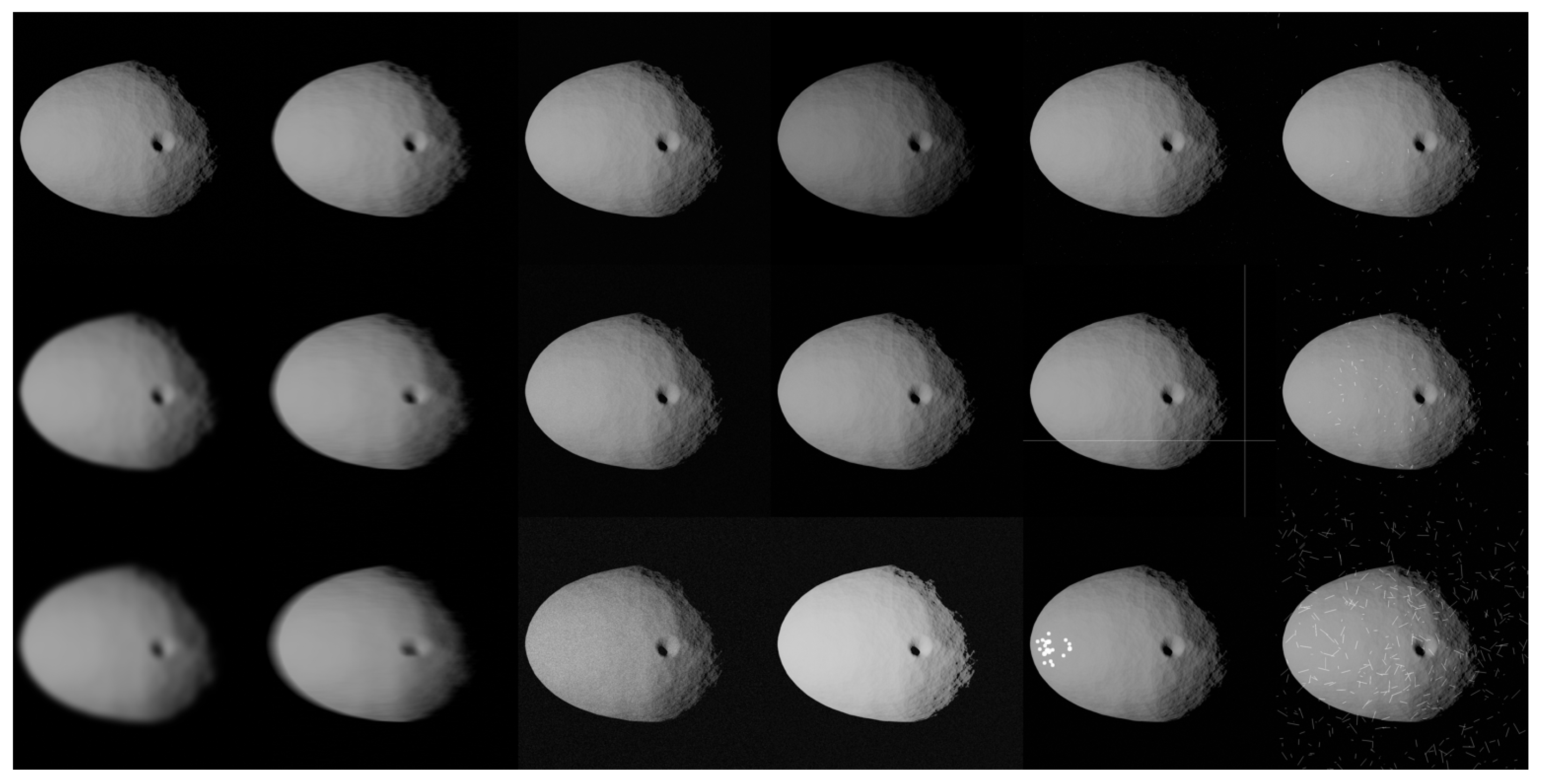
| Img Name | Rendering | Noise | SSIM | ID |
|---|---|---|---|---|
| N20160128T002344268ID20F71 | 0.7537 | 1,1 | ||
| N20160130T173323717ID20F22 | 0.4421 | 1,3 | ||
| W20150316T053347931ID20F13 | 0.9360 | 2,1 | ||
| W20160617T102200832ID20F18 | 0.8920 | 2,3 | ||
| FC21A0037273_15136172940F1E | 0.4430 | 3,1 | ||
| FC21A0037405_15157034032F3I | 0.3979 | 3,3 | ||
| FC21A0037589_15158013232F1I | 0.3558 | 4,1 | ||
| FC21A0037593_15158020232F1I | 0.4973 | 4,3 | ||
| FC21A0037978_15163064254F1G | 0.2870 | 5,1 | ||
| FC21A0038693_15172150728F6G | 0.3557 | 5,3 | ||
| FC21A0038787_15173122643F1G | 0.3379 | 6,1 | ||
| FC21A0039042_15176210244F1H | 0.6744 | 6,3 | ||
| FC21B0003258_11205095604F6C | 0.7201 | 7,1 | ||
| FC21B0003428_11205235222F5C | 0.8499 | 7,3 | ||
| FC21B0003757_11218102757F7D | 0.7034 | 8,1 | ||
| FC21B0003866_11218121551F4D | 0.8337 | 8,3 | ||
| FC21B0004630_11226232738F7D | 0.6480 | 9,1 | ||
| FC21B0005299_11230130409F6B | 0.8114 | 9,3 | ||
| FC21B0005871_11232204234F4B | 0.6644 | 10,1 | ||
| FC21B0006422_11238100914F1B | 0.8142 | 10,3 |
| Img Name | Rendering | Noise | SSIM | ID |
|---|---|---|---|---|
| 20181211T181336S699_map_specradL2b | 0.9200 | 1,2 | ||
| 0.9187 | 1,3 | |||
| 0.9458 | 1,4 | |||
| 20181212T043459S572_map_specradL2x | 0.8054 | 2,2 | ||
| 0.8046 | 2,3 | |||
| 0.8958 | 2,4 | |||
| 20181212T064255S344_map_radL2pan | 0.7090 | 3,2 | ||
| 0.7078 | 3,3 | |||
| 0.8549 | 3,4 | |||
| 20181212T085936S404_map_iofL2pan | 0.7131 | 4,2 | ||
| 0.7165 | 4,3 | |||
| 0.8459 | 4,4 | |||
| 20181213T043620S487_map_radL2pan | 0.7537 | 5,2 | ||
| 0.7528 | 5,3 | |||
| 0.8175 | 5,4 | |||
| 20181215T053926S725_map_iofL2b | 0.9339 | 6,2 | ||
| 0.9337 | 6,3 | |||
| 0.9473 | 6,4 | |||
| 20181217T033612S897_map_iofL2pan | 0.8127 | 7,2 | ||
| 0.8107 | 7,3 | |||
| 0.8845 | 7,4 |
Disclaimer/Publisher’s Note: The statements, opinions and data contained in all publications are solely those of the individual author(s) and contributor(s) and not of MDPI and/or the editor(s). MDPI and/or the editor(s) disclaim responsibility for any injury to people or property resulting from any ideas, methods, instructions or products referred to in the content. |
© 2023 by the authors. Licensee MDPI, Basel, Switzerland. This article is an open access article distributed under the terms and conditions of the Creative Commons Attribution (CC BY) license (https://creativecommons.org/licenses/by/4.0/).
Share and Cite
Pugliatti, M.; Buonagura, C.; Topputo, F. CORTO: The Celestial Object Rendering TOol at DART Lab. Sensors 2023, 23, 9595. https://doi.org/10.3390/s23239595
Pugliatti M, Buonagura C, Topputo F. CORTO: The Celestial Object Rendering TOol at DART Lab. Sensors. 2023; 23(23):9595. https://doi.org/10.3390/s23239595
Chicago/Turabian StylePugliatti, Mattia, Carmine Buonagura, and Francesco Topputo. 2023. "CORTO: The Celestial Object Rendering TOol at DART Lab" Sensors 23, no. 23: 9595. https://doi.org/10.3390/s23239595