

Assessment of Number of Critical Satellites for Ground-Based Augmentation System Continuity Allocation to Support Category II/III Precision Approaches
Abstract
:1. Introduction
2. GBAS Protection Level
2.1. GBAS Protection Level Equations
2.2. Consideration of DV and DL for GASTs D and D1
2.2.1. The Impact of the Ionospheric Delay
2.2.2. The Impact of the Noise and Multipath
- Input: White Gaussian Noise (WGN)
- Input: first-order Gauss–Markov (GM) process
- Determination of and to compute the variance of
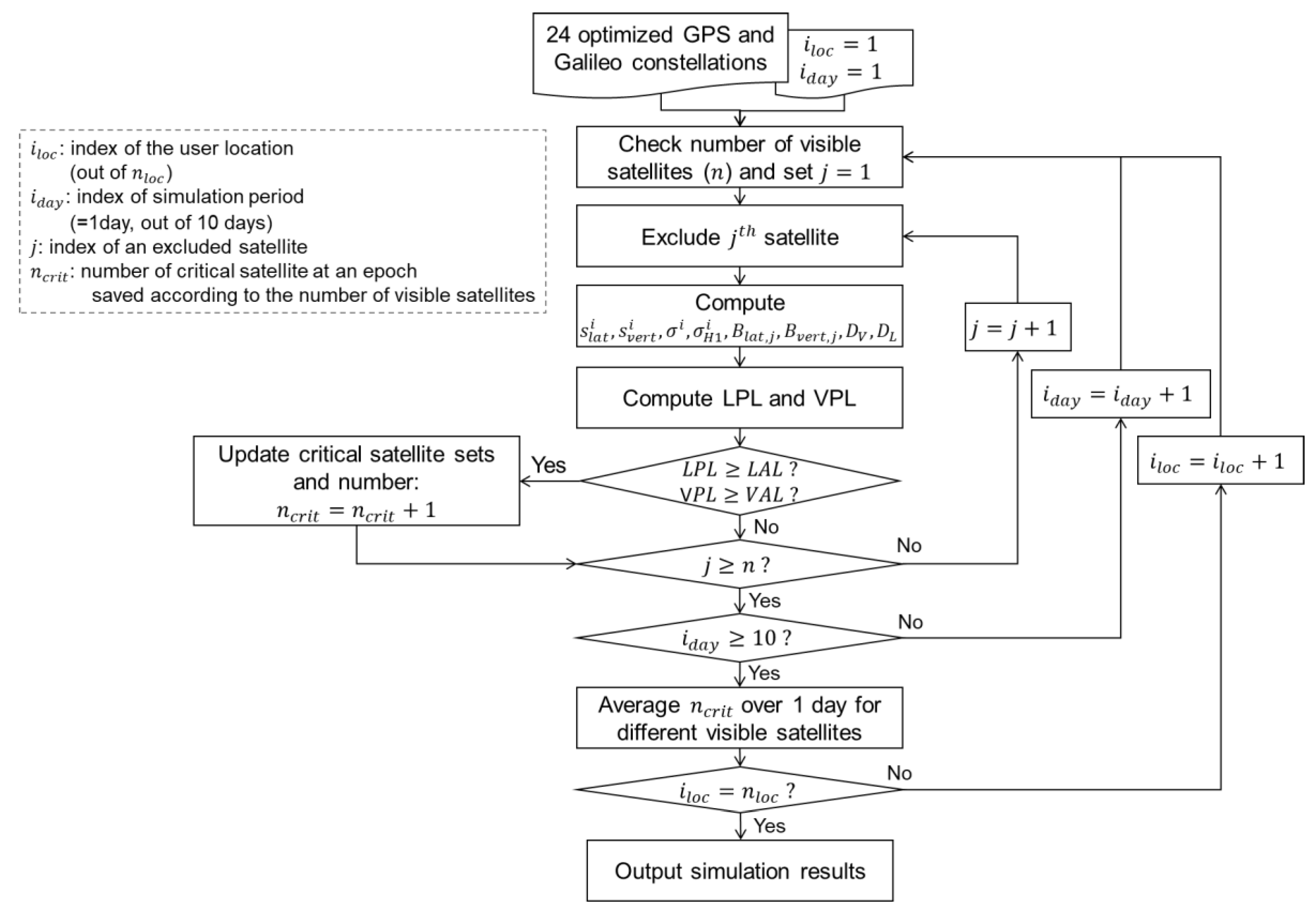
3. Methodology
4. Results
5. Discussion
6. Conclusions
Author Contributions
Funding
Informed Consent Statement
Data Availability Statement
Conflicts of Interest
Appendix A
References
- ICAO Annex 6 Operation of Aircraft. Part I—International Commercial Air Transport, 12th ed.; International Standards and Recommended Practices: Quebec, Canada, 2020.
- ICAO Annex 10 Radio Navigation Aids, Vol. 1, Amendments 91, 7th ed.; International Standards and Recommended Practices: Quebec, Canada, 2018.
- ICAO Navigation System Panel (NSP). GBAS CAT II/III Development Baseline SARPs. 2009. Available online: http://www.icao.int/safety/airnavigation/documents/gnss_cat_ii_iii.pdf (accessed on 23 January 2023).
- Murphy, T.; Harris, M.; Balvedi, G.; McGraw, G.; Wichgers, J.; Lavik, L.; Topland, M.; Tuffaha, M.; Saito, S. Managing Long Time Constant and Variable Rate Carrier Smoothing for DFMC GBAS. In Proceedings of the 36th International Technical Meeting of the Satellite Division of The Institute of Navigation (ION GNSS+ 2023), Denver, CO, USA, 11–15 September 2023. [Google Scholar]
- Caamano, M.; Gerbeth, D. L5/E5a-Based Fallback Mode for Dual-Frequency Multi-Constellation GBAS. In Proceedings of the 36th International Technical Meeting of the Satellite Division of The Institute of Navigation (ION GNSS+ 2023), Denver, CO, USA, 11–15 September 2023. [Google Scholar]
- SESAR.SESAR2020 PJ14 Final Project Report, H2020-SESAR-2015/2. 2019. Available online: https://sesarju.paddlecms.net/sites/default/files/documents/projects/FPR/SESAR2020_PJ14_D1.pdf (accessed on 30 August 2020).
- Pullen, S. Augmented GNSS: Fundamentals and Keys to Integrity and Continuity. Proceeding of the ION GNSS 2012, Nashville, TN, USA, 17–21 September 2012. [Google Scholar]
- RTCA. DO-245, Minimum Aviation System Performance Standards (MOPS) for the Local Area Augmentation System (LAAS); Radio Technical Commission for Aeronautics: Washington DC, USA, 2004. [Google Scholar]
- Kline, P.; Murphy, T.; Van Dyke, K. LAAS Availability Assessment: The Effects of Augmentations and Critical Satellites on Service Availability. In Proceedings of the 11th International Technical Meeting of the Satellite Division of The Institute of Navigation (ION GPS 1998), Nashville, TN, USA, 15–18 September 1998; pp. 503–516. [Google Scholar]
- Zhai, Y.; Joerger, M.; Pervan, B. Bounding continuity risk in H-ARAIM FDE. In Proceedings of the ION 2017 Pacific PNT Meeting, Honolulu, HI, USA, 1–4 May 2017; pp. 20–35. [Google Scholar]
- RTCA. DO-253D, Minimum Operational Performance Standards (MOPS) for GPS Local Area Augmentation System Airborne Equipment; Radio Technical Commission for Aeronautics: Washington DC, USA, 2008. [Google Scholar]
- Shively, C.A.; Hsiao, T.T. Availability of GAST D GBAS Considering Continuity of Airborne Monitors. In Proceedings of the 2010 International Technical Meeting of The Institute of Navigation, San Diego, CA, USA, 25–27 January 2010; pp. 365–375. [Google Scholar]
- Hwang, P.Y.; McGraw, G.A.; Bader, J.R. Enhanced Differential GPS Carrier-Smoothed Code Processing Using Du-al-Frequency Measurements. Navigation 1999, 46, 127–137. [Google Scholar] [CrossRef]
- McGraw, G.A.; Murphy, T.; Brenner, M.; Pullen, S.; Van Dierendonck, A.J. Development of the LAAS Accuracy Models. In Proceedings of the ION GPS 2000, Salt Lake City, UT, USA, 19–22 September 2000; pp. 1212–1223. [Google Scholar]
- Lee, J.; Pullen, S.; Datta-Barua, S.; Enge, P. Assessment of Ionosphere Spatial Decorrelation for Global Positioning System-Based Aircraft Landing Systems. J. Aircr. 2007, 44, 1662–1669. [Google Scholar] [CrossRef]
- Guilbert, A. Optimal GPS/Galileo GBAS Methodologies with an Application to Troposphere. Ph.D. Thesis, Université de Toulouse, Toulouse, France, 2016. [Google Scholar]
- Blanch, J.; Walter, T.; Phelts, R.E. Development and Evaluation of Airborne Multipath Error Bounds for L1-L5. In Proceedings of the 2019 International Technical Meeting of The Institute of Navigation, Reston, VA, USA, 28–31 January 2019; pp. 53–61. [Google Scholar] [CrossRef]
- Gardner, W.A. Introduction to Random Processes with Applications to Signals & Systems, 2nd ed.; McGraw-Hill: New York, NY, USA, 1990. [Google Scholar]
- Pervan, B.; Khanafseh, S.; Patel, J. Test Statistic Auto- and Cross-correlation Effects on Monitor False Alert and Missed Detection Probabilities. In Proceedings of the 2017 International Technical Meeting of The Institute of Navigation, Monterey, CA, USA, 30 January–2 February 2017; pp. 562–590. [Google Scholar] [CrossRef]
- RTCA. DO-229E, Minimum Operational Performance Standards (MOPS) for GPSWAAS Airborne Equipment; Radio Technical Commission for Aeronautics: Washington DC, USA, 2016. [Google Scholar]
- WG-C Advanced RAIM Technical Subgroup. Reference Airborne Algorithm Description Document (ADD), (Version 3.1). ARAIM TSG. 2019. Available online: http://web.stanford.edu/group/scpnt/gpslab/website_files/maast/maast_araimpb0.3.zip (accessed on 1 September 2021).
- Blanch, J.; Walter, T.; Milner, C.; Joerger, M.; Pervan, B.; Bouvet, D. Baseline Advanced RAIM User Algorithm: Proposed Updates. In Proceedings of the 2022 International Technical Meeting of The Institute of Navigation, Long Beach, CA, USA, 25–27 January 2022; pp. 229–251. [Google Scholar] [CrossRef]
- Gratton, L.; Joerger, M.; Pervan, B. Carrier Phase Relative RAIM Algorithms and Protection Level Derivation. J. Navig. 2010, 63, 215–231. [Google Scholar] [CrossRef]
- Lee, H.; Pullen, S.; Lee, J.; Park, B.; Yoon, M.; Seo, J. Optimal Parameter Inflation to Enhance the Availability of Single-Frequency GBAS for Intelligent Air Transportation Systems. IEEE Trans. Intell. Transp. 2022, 23, 17801–17808. [Google Scholar] [CrossRef]
- Beidleman, S.W. GPS Versus Galileo: Balancing for Position in Space; Air University Press: Montgomery, AL, USA, 2006. [Google Scholar]
- Song, J.; Milner, C.; Macabiau, C.; No, H.; Estival, P. Feasibility Analysis of GBAS/INS and RRAIM Integration for Surface Movement Operation. In Proceedings of the 34th International Technical Meeting of the Satellite Division of The Institute of Navigation (ION GNSS+ 2021), St. Louis, MI, USA, 20–24 September 2021; pp. 1469–1480. [Google Scholar]
- Official, U.S. Government Information about the Global Positioning System (GPS) and Related Topics. Available online: https://www.gps.gov/systems/gps/space/ (accessed on 3 October 2023).


| References | Types of Augmentation System and Supported Approach | Remarks |
|---|---|---|
| Pullen [7] | GBAS, CAT I (CAST C) | - Nc assessed |
| ICAO SARPs [3] | GBAS, CAT II/III (GAST D) | - Nc assessed - Simulation condition not provided |
| Kline et al. [9] | GBAS; CATs I, II, III | - Nc not assessed - Only the impact of hypothetical Nc on the availability analyzed |
| Zhai et al. [10] | ARAIM, RNP 0.1 and 0.3 | - Nc and corresponding continuity requirement of SV loss dynamically assessed and allocated - Not applicable to GBAS |
| Flight Phase Layout | ||
| Parameters | DH = 200 ft to Threshold | Threshold to Roll Out |
| Glide Path Angle (GPA) | 2.5 degrees [3] | |
(Distance from GND 1 to threshold) | 5 km [16] | |
| Residual ionospheric uncertainty | ||
| Parameters | DH = 200 ft to threshold | Threshold to roll out |
(Vertical ionosphere gradient) | 4 mm/km [14,15] 8 mm/km [8] | |
(Slant range distance from an aircraft location and a reference point) | ||
(Speed of the aircraft) | 161 knots (82.83 m/s) [16] | |
| Residual tropospheric uncertainty | ||
| Parameters | DH = 200 ft to threshold | Threshold to roll out |
(Refractivity uncertainty) | 33 [16] | |
(Tropospheric scale height) | 15730 m [16] | |
(Difference of altitude between an aircraft and the GND 1 subsystem) | 200 ft | 0 |
| Receiver error model | ||
| Parameters | DH = 200 ft to threshold | Threshold to roll out |
(Airborne receiver model: AAD B, AMD B) | [8] [8] | |
(Ground receiver model: GAD 2 C) | [8] | |
(Time constant of the ground multipath) | 6 s [19] | |
(Time constant of the airborne multipath) | 7 s [19] | |
| Number of Satellites in View | GAST D1 with GPS L1 | Number of Satellites in View | GAST D1 with Galileo E1 | ||||||
|---|---|---|---|---|---|---|---|---|---|
| DH = 200 ft to Threshold | Threshold to Roll Out | DH = 200 ft to Threshold | Threshold to Roll Out | ||||||
| (mm/km) | (mm/km) | ||||||||
| 4 | 8 | 4 | 8 | 4 | 8 | 4 | 8 | ||
| 4 | 4 (by definition) | 4 | 4 (by definition) | ||||||
| 5 | 2.4430 | 2.9772 | 2.2769 | 2.6091 | 5 | NA | NA | NA | NA |
| 6 | 0.8113 | 0.9266 | 0.7658 | 0.8652 | 6 | 0.0000 | 0.0000 | 0.0000 | 0.0000 |
| 7 | 0.2095 | 0.2663 | 0.1903 | 0.2436 | 7 | 0.0010 | 0.0010 | 0.0010 | 0.0010 |
| 8 | 0.0801 | 0.1092 | 0.0722 | 0.1001 | 8 | 0.0050 | 0.0277 | 0.0033 | 0.0201 |
| 9 | 0.0535 | 0.0711 | 0.0502 | 0.0661 | 9 | 0.0000 | 0.0000 | 0.0000 | 0.0000 |
| 10 or more | 0.0000 | 0.0000 | 0.0000 | 0.0000 | 10 or more | 0.0000 | 0.0000 | 0.0000 | 0.0000 |
| Number of Satellites in View | GAST E, DC (GPS/Galileo SF, DF) | Number of Satellites in View | GAST E, SC (GPS SF, DF) | ||||||
|---|---|---|---|---|---|---|---|---|---|
| DH = 200 ft to Threshold | Threshold to Roll Out | DH = 200 ft to Threshold | Threshold to Roll Out | ||||||
| DF | SF | DF | SF | DF | SF | DF | SF | ||
| 5 | 5 (by definition) | 4 | 4 (by definition) | ||||||
| 6 to 12 | 0.0000 | 0.0000 | 0.0000 | 0.0000 | 5 | 3.9902 | 1.3485 | 3.9055 | 1.3257 |
| 13 | 0.0000 | 0.0000 | 0.0000 | 0.0000 | 6 | 1.6407 | 0.1654 | 1.5496 | 0.1533 |
| 14 | 0.0000 | 0.0000 | 0.0000 | 0.0000 | 7 | 0.5711 | 0.0232 | 0.5304 | 0.0220 |
| 15 or more | 0.0000 | 0.0000 | 0.0000 | 0.0000 | 8 | 0.2563 | 0.0031 | 0.2359 | 0.0026 |
| 9 | 0.1825 | 0.0021 | 0.1720 | 0.0019 | |||||
| 10 or more | 0.0078 | 0.0000 | 0.0063 | 0.0000 | |||||
| Number of Satellites in View | GAST E, DC (GPS/Galileo SF, DF) | Number of Satellites in View | GAST E, SC (GPS SF, DF) | ||||||
|---|---|---|---|---|---|---|---|---|---|
| DH = 200 ft to Threshold | Threshold to Roll Out | DH = 200 ft to threshold | Threshold to Roll Out | ||||||
| DF | SF | DF | SF | DF | SF | DF | SF | ||
| 5 | 5 (by definition) | 4 | 4 (by definition) | ||||||
| 6 to 12 | 0.0000 | 0.0000 | 0.0000 | 0.0000 | 5 | 3.9902 | 1.9088 | 3.9055 | 1.8860 |
| 13 | 0.0000 | 0.0000 | 0.0000 | 0.0000 | 6 | 1.6407 | 0.5491 | 1.5496 | 0.5237 |
| 14 | 0.0000 | 0.0000 | 0.0000 | 0.0000 | 7 | 0.5711 | 0.1230 | 0.5304 | 0.1156 |
| 15 or more | 0.0000 | 0.0000 | 0.0000 | 0.0000 | 8 | 0.2563 | 0.0614 | 0.2359 | 0.0578 |
| 9 | 0.1825 | 0.0489 | 0.1720 | 0.0461 | |||||
| 10 or more | 0.0078 | 0.0000 | 0.0063 | 0.0000 | |||||
Disclaimer/Publisher’s Note: The statements, opinions and data contained in all publications are solely those of the individual author(s) and contributor(s) and not of MDPI and/or the editor(s). MDPI and/or the editor(s) disclaim responsibility for any injury to people or property resulting from any ideas, methods, instructions or products referred to in the content. |
© 2023 by the authors. Licensee MDPI, Basel, Switzerland. This article is an open access article distributed under the terms and conditions of the Creative Commons Attribution (CC BY) license (https://creativecommons.org/licenses/by/4.0/).
Share and Cite
Song, J.; Milner, C. Assessment of Number of Critical Satellites for Ground-Based Augmentation System Continuity Allocation to Support Category II/III Precision Approaches. Sensors 2023, 23, 8273. https://doi.org/10.3390/s23198273
Song J, Milner C. Assessment of Number of Critical Satellites for Ground-Based Augmentation System Continuity Allocation to Support Category II/III Precision Approaches. Sensors. 2023; 23(19):8273. https://doi.org/10.3390/s23198273
Chicago/Turabian StyleSong, Junesol, and Carl Milner. 2023. "Assessment of Number of Critical Satellites for Ground-Based Augmentation System Continuity Allocation to Support Category II/III Precision Approaches" Sensors 23, no. 19: 8273. https://doi.org/10.3390/s23198273