
An Efficient Brain Tumor Segmentation Method Based on Adaptive Moving Self-Organizing Map and Fuzzy K-Mean Clustering
 , , , , ,
Abstract
:1. Introduction
- This research aims to suggest an automated workflow that can automatically accurately identify and classify brain tumors. The proposed model’s initial training images were compiled using the GLCM feature extraction method. One of the most well-known feature extraction techniques is GLCM, which can determine the textural connection among an image’s pixels;
- This research utilizes the online Kaggle brain tumor dataset;
- An FKM is used to distinguish the tumor region from the surrounding tissue;
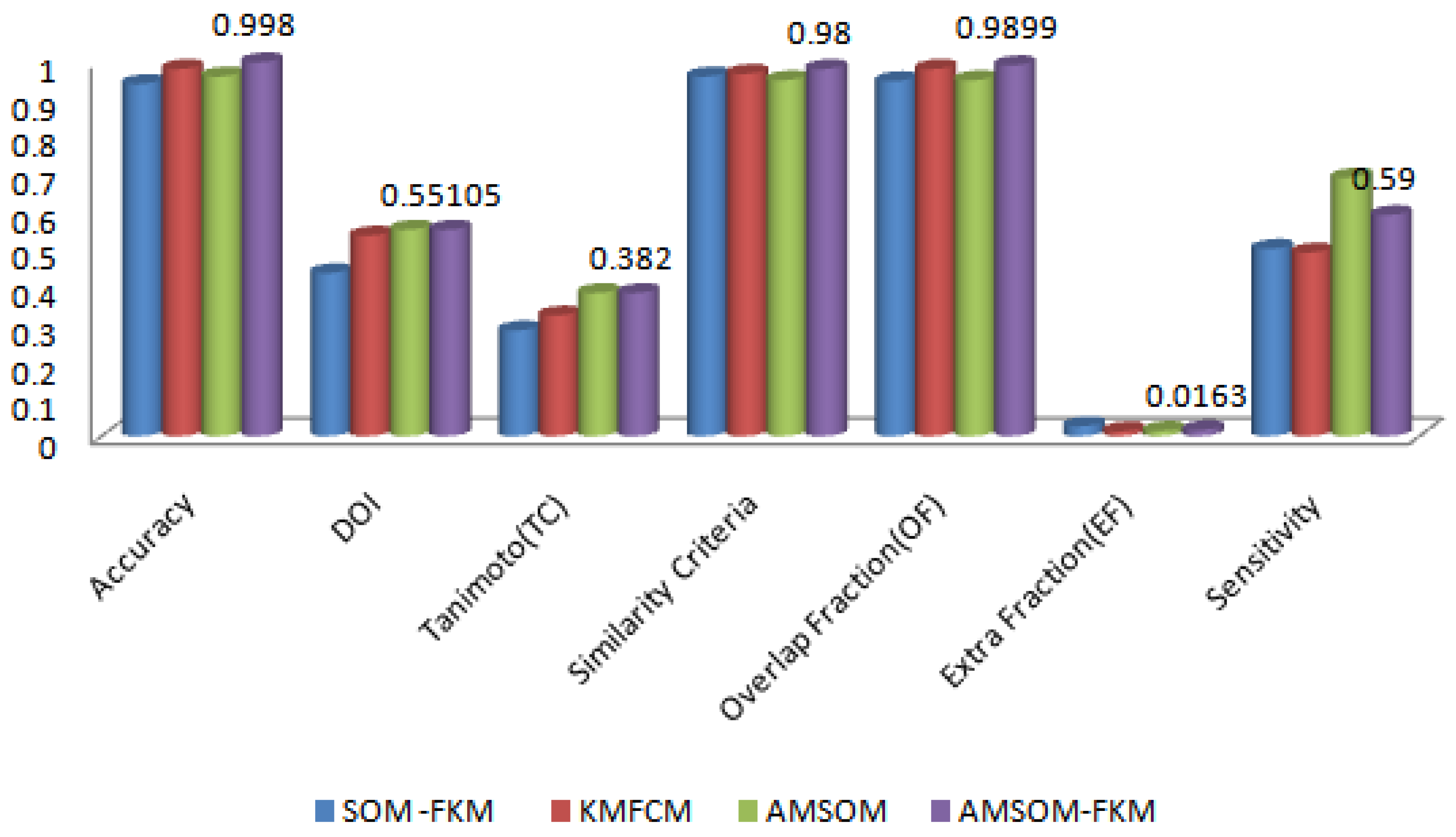
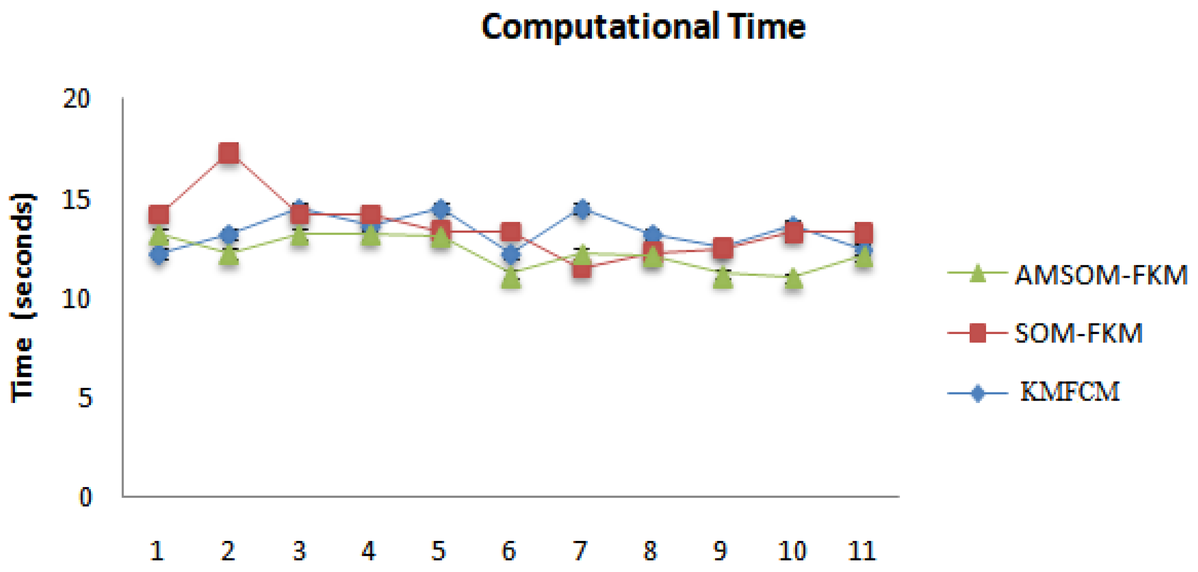
- The proposed AMSOM-FKM technique and existing methods, i.e., Fuzzy-C-means and K-mean (FMFCM), hybrid self-organization mapping-FKM, were implemented over MATLAB and compared based on comparison parameters, i.e., sensitivity, precision, accuracy, and similarity index values;
- The proposed model achieves better precision, accuracy, and sensitivity than existing methods.
2. Related Work
3. Materials and Methods
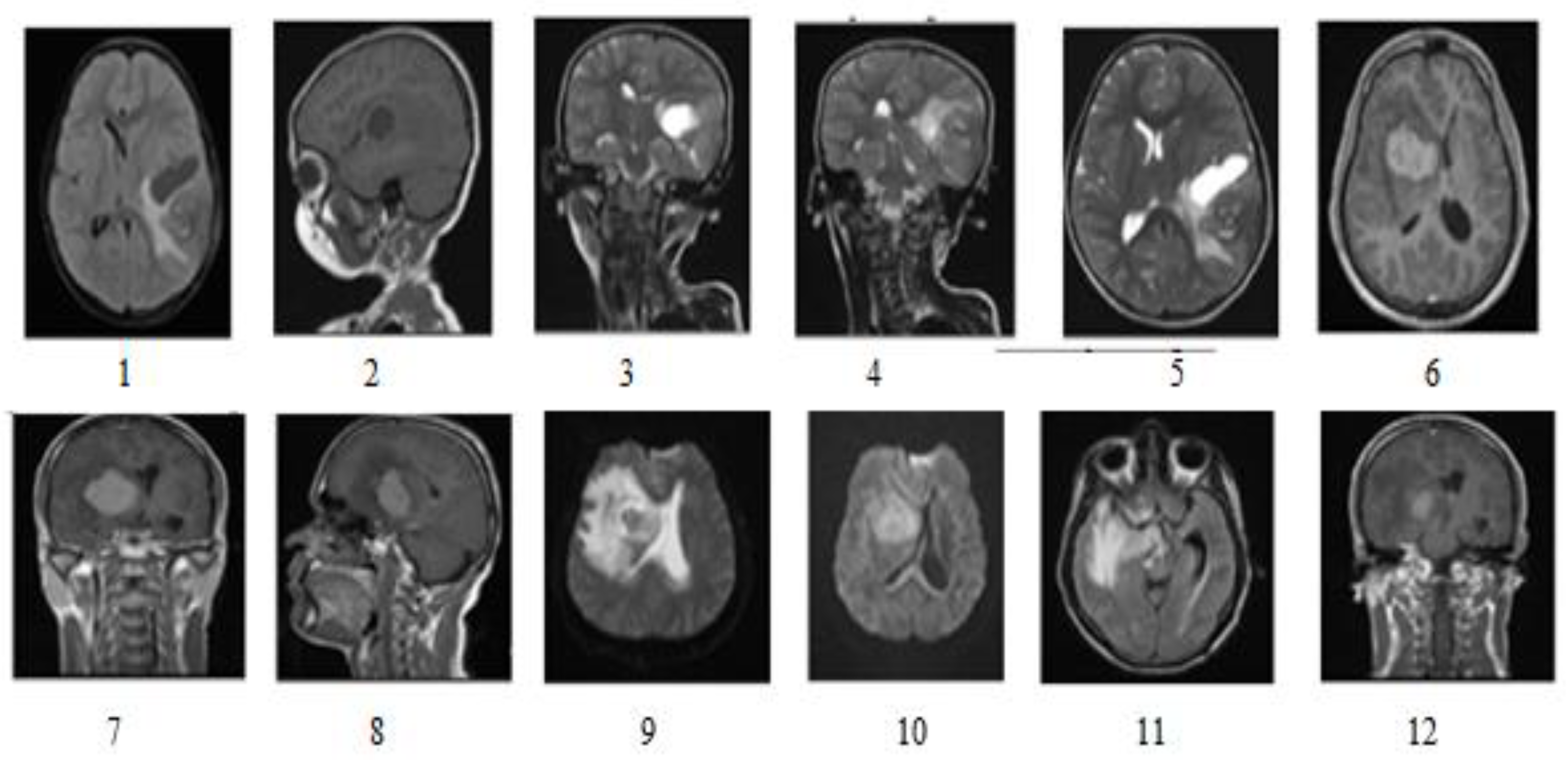
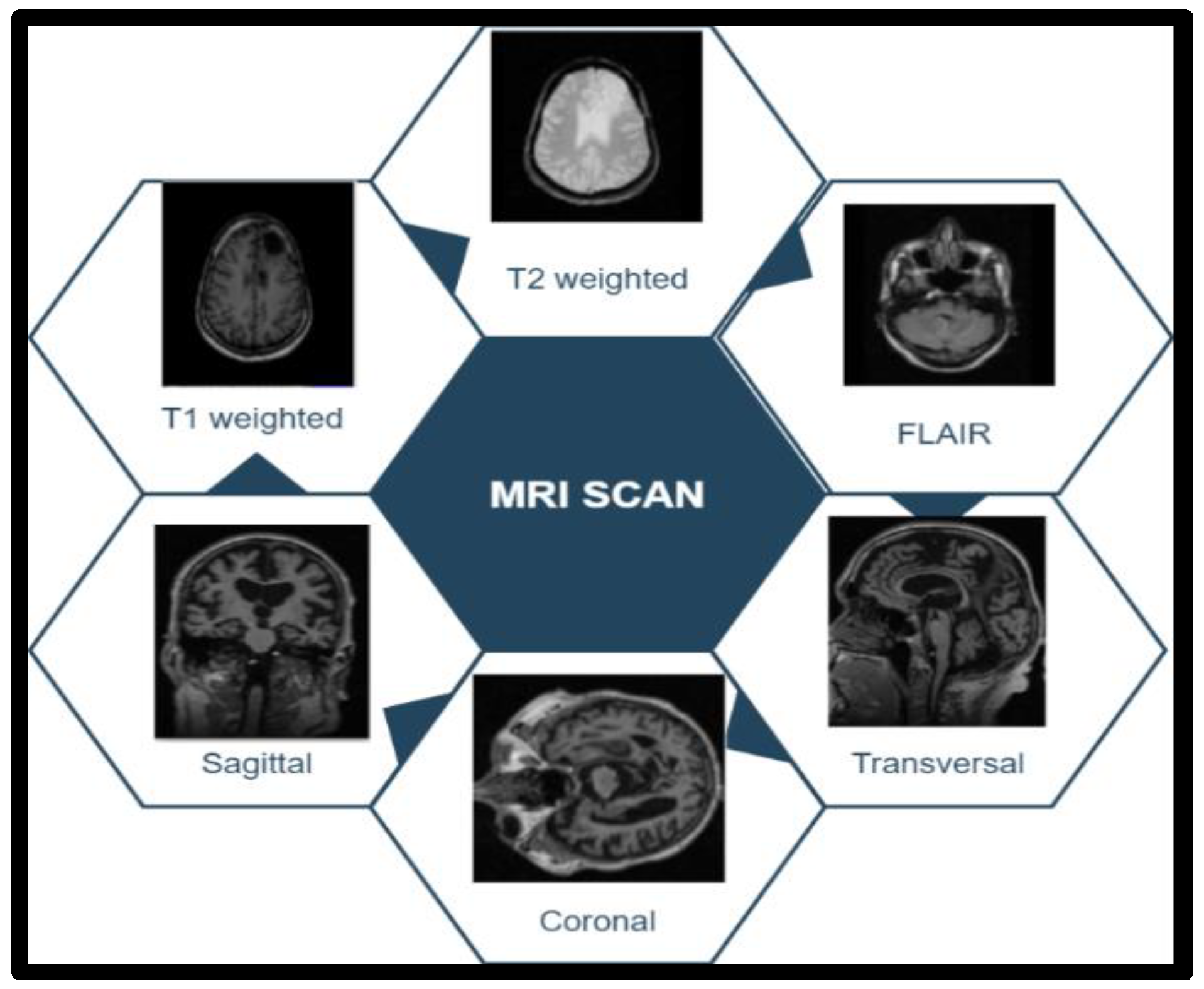
3.1. Dataset
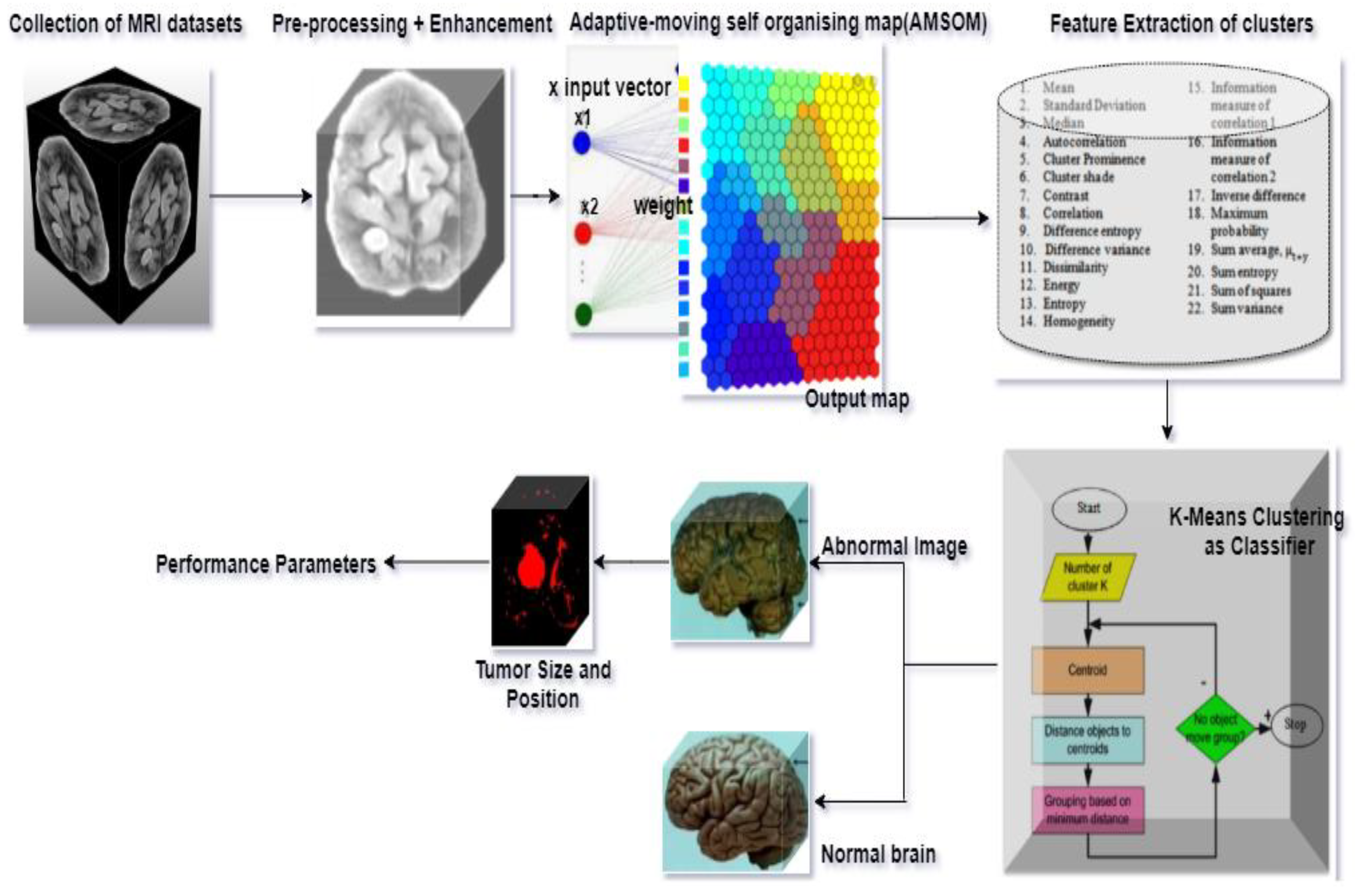
3.2. Proposed Method
3.2.1. Pre-Processing
3.2.2. Image Enhancement
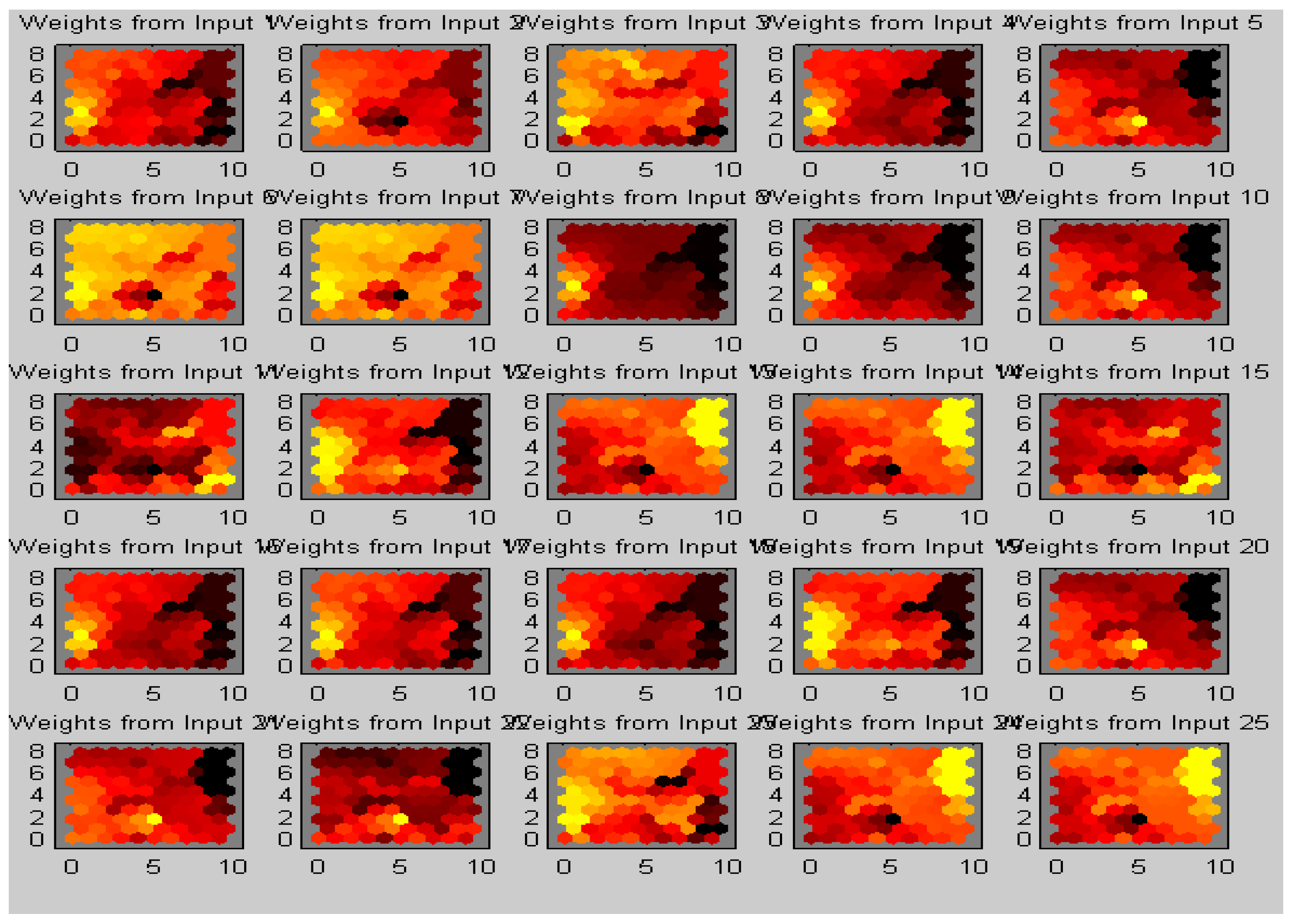
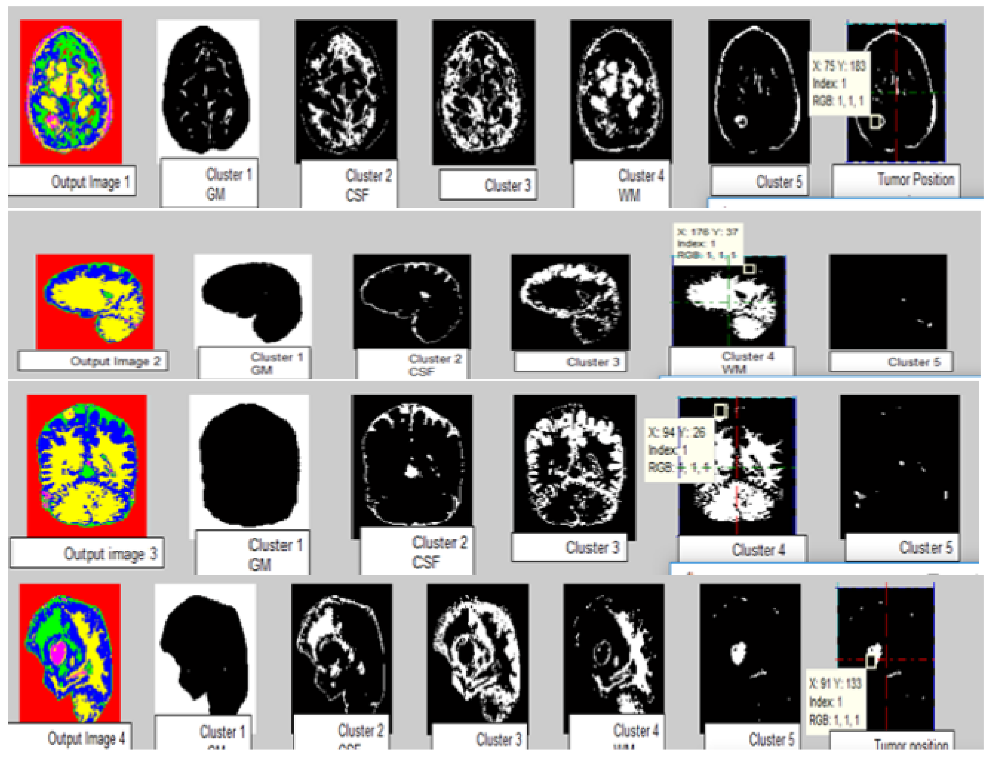
3.2.3. Clustering
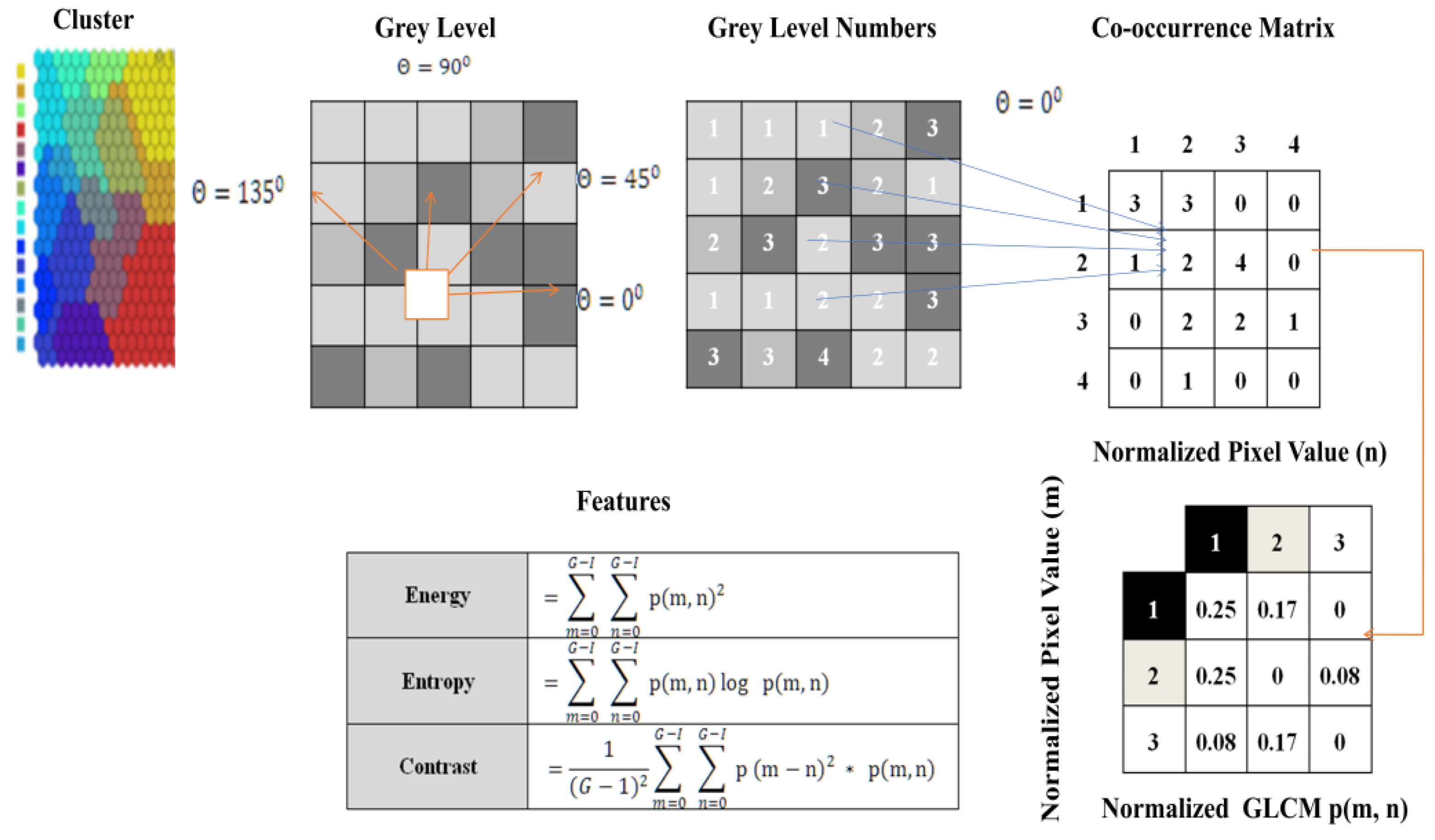
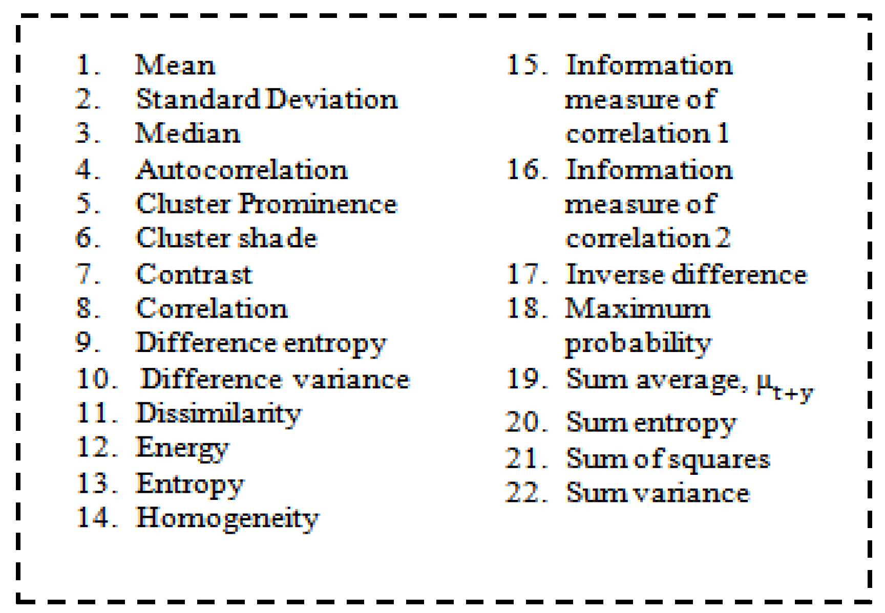
3.2.4. Feature Extraction
3.3. Classification
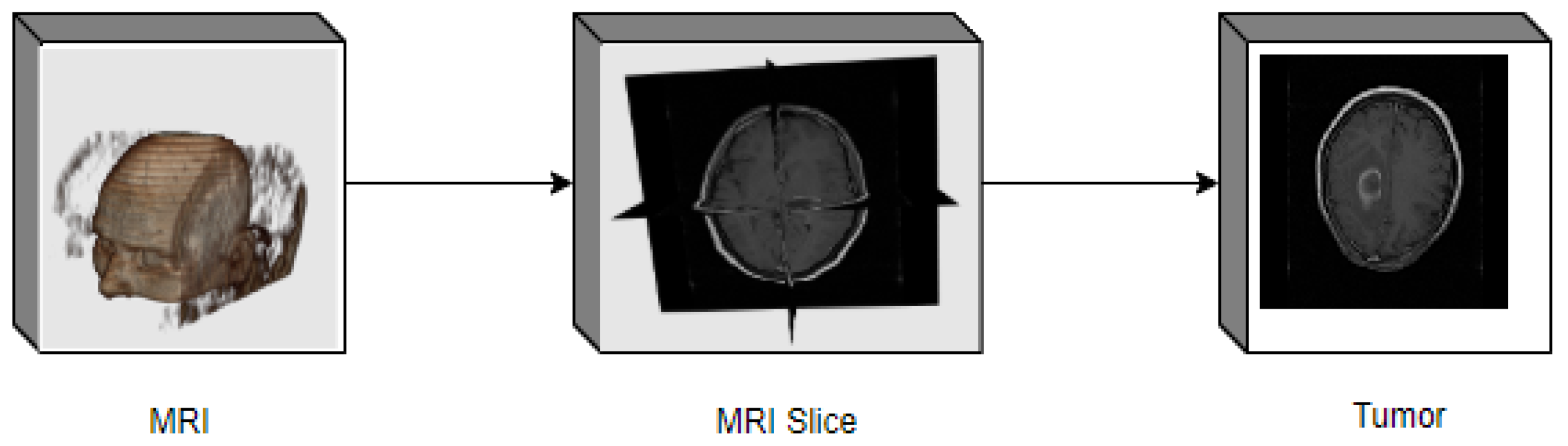
3.4. Volume Estimation
3.5. Performance Parameters
3.6. Proposed AMSOM-FKM Algorithm
| Algorithm 1 Proposed AMSOM-FKM Algorithm |
| Input: MRI image dataset Output: Tumor and non-tumor images
|
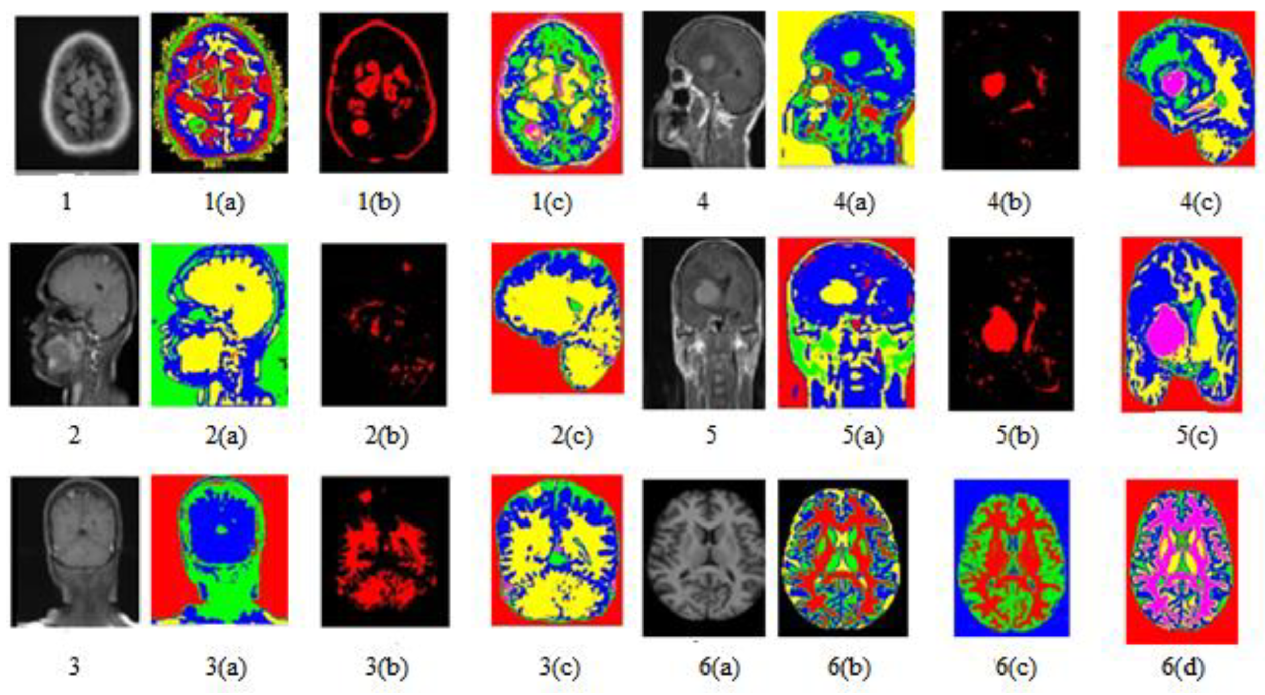
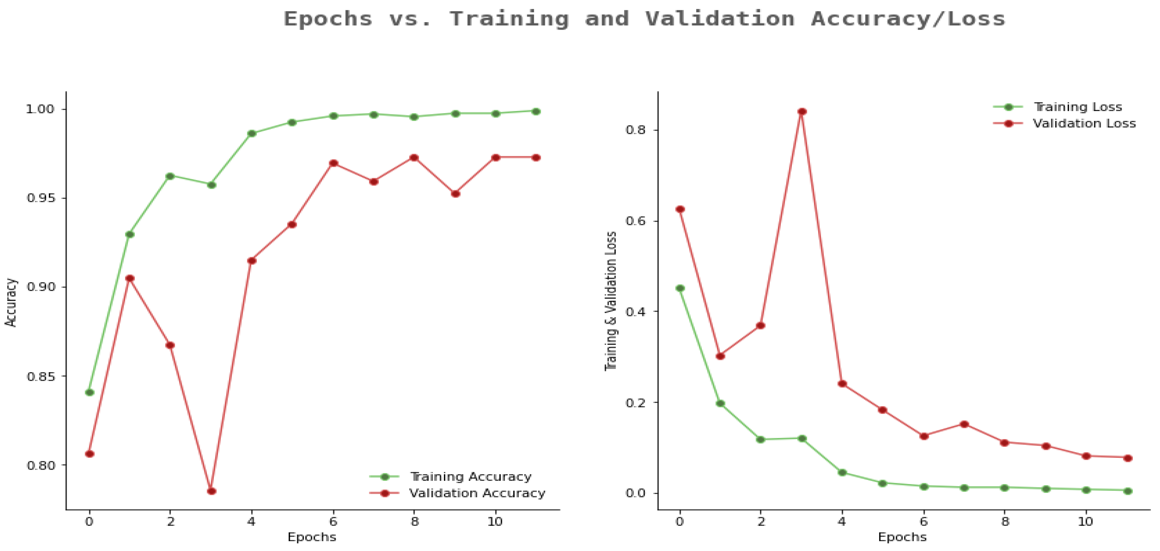
4. Result and Analysis
5. Conclusions and Future Work
Author Contributions
Funding
Institutional Review Board Statement
Informed Consent Statement
Data Availability Statement
Conflicts of Interest
References
- Turk, O.; Ozhan, D.; Acar, E.; Akinci, T.C.; Yilmaz, M. Automatic detection of brain Tumors with the aid of ensemble deep learning architectures and class activation map indicators by employing magnetic resonance images. Z. Med. Physik. 2023, in press. [CrossRef]
- Ahuja, S.; Panigrahi, B.K.; Gandhi, T.K. Enhanced performance of Dark-Nets for brain Tumor classification and segmentation using colormap-based superpixel techniques. Mach. Learn. Appl. 2022, 7, 100212. [Google Scholar] [CrossRef]
- Shanthi, S.; Saradha, S.; Smitha, J.A.; Prasath, N.; Anandakumar, H. An efficient automatic brain Tumor classification using optimized hybrid deep neural network. Int. J. Intell. Netw. 2022, 3, 188–196. [Google Scholar] [CrossRef]
- Vankdothu, R.; Hameed, M.A. Brain Tumor segmentation of MR images using SVM and fuzzy classifier in machine learning. Meas. Sens. 2022, 24, 100440. [Google Scholar] [CrossRef]
- Walsh, J.; Othmani, A.; Jain, M.; Dev, S. Using U-Net network for efficient brain Tumor segmentation in MRI images. Healthc. Anal. 2022, 2, 100098. [Google Scholar] [CrossRef]
- Anaya-Isaza, A.; Mera-Jimenez, L. Data Augmentation and Transfer Learning for Brain Tumor Detection in Magnetic Resonance Imaging. IEEE Access 2022, 10, 23217–23233. [Google Scholar] [CrossRef]
- Lu, S.L.; Liao, H.C.; Hsu, F.M.; Liao, C.C.; Lai, F.; Xiao, F. The intracranial Tumor segmentation challenge: Contour Tumors on brain MRI for radiosurgery. Neuroimage 2021, 244, 118585. [Google Scholar] [CrossRef]
- Deshpande, A.; Estrela, V.V.; Patavardhan, P. The DCT-CNN-ResNet50 architecture to classify brain Tumors with super-resolution, convolutional neural network, and the ResNet50. Neurosci. Inform. 2021, 1, 100013. [Google Scholar] [CrossRef]
- Onyema, E.M.; Shukla, P.K.; Dalal, S.; Mathur, M.N.; Zakariah, M.; Tiwari, B. Enhancement of patient facial recognition through deep learning algorithm: ConvNet. J. Healthc. Eng. 2021, 6, 2021. [Google Scholar] [CrossRef]
- Majib, M.S.; Rahman, M.M.; ShahriarSazzad, T.M.; Khan, N.I.; Dey, S.K. VGG-SCNet: A VGG Net based Deep Learning framework for Brain Tumor Detection on MRI Images. IEEE Access 2021, 9, 116942–116952. [Google Scholar] [CrossRef]
- Wang, W.; Bu, F.; Lin, Z.; Zhai, S. Learning Methods of Convolutional Neural Network Combined with Image Feature Extraction in Brain Tumor Detection. IEEE Access 2020, 8, 152659–152668. [Google Scholar] [CrossRef]
- Noreen, N.; Palaniappan, S.; Qayyum, A.; Ahmad, I.; Imran, M.; Shoaib, M. A Deep Learning Model Based on Concatenation Approach for the Diagnosis of Brain Tumor. IEEE Access 2020, 8, 55135–55144. [Google Scholar] [CrossRef]
- Kumar Mallick, P.; Ryu, S.H.; Satapathy, S.K.; Mishra, S.; Nguyen, G.N.; Tiwari, P. Brain MRI Image Classification for Cancer Detection Using Deep Wavelet Autoencoder-Based Deep Neural Network. IEEE Access 2019, 7, 46278–46287. [Google Scholar] [CrossRef]
- Song, G.; Huang, Z.; Zhao, Y.; Zhao, X.; Liu, Y.; Bao, M.; Han, J.; Li, P. A Noninvasive System for the Automatic Detection of Gliomas Based on Hybrid Features and PSO-KSVM. IEEE Access 2019, 7, 13842–13855. [Google Scholar] [CrossRef]
- Li, M.; Kuang, L.; Xu, S.; Sha, Z. Brain Tumor Detection Based on Multimodal Information Fusion and Convolutional Neural Network. IEEE Access 2019, 7, 180134–180146. [Google Scholar] [CrossRef]
- Alam, M.S.; Rahman, M.M.; Hossain, M.A.; Islam, M.K.; Ahmed, K.M.; Ahmed, K.T.; Miah, M.S. Automatic human brain Tumor detection in MRI image using template-based K means and improved fuzzy C means clustering algorithm. Big Data Cogn. Comput. 2019, 3, 27. [Google Scholar] [CrossRef]
- Aslam, A.; Khan, E.; Beg, M.M.S. Improved edge detection algorithm for brain Tumor segmentation. In Proceedings of the Second International Symposium on Computer Vision and the Internet (VisionNet’15), Kerala, India, 10–13 August 2015. [Google Scholar]
- Chanchlani, A.; Chaudhari, M.; Shewale, B.; Jha, A. Tumor detection in brain MRI using Clustering and segmentation algorithm. Imp. J. Interdiscip. Res. 2017, 3, 2122–2127. [Google Scholar]
- Lakra, A.; Dubey, R.B. A comparative analysis of MRI brain Tumor segmentation technique. Int. J. Comput. Appl. 2015, 125, 5–14. [Google Scholar] [CrossRef]
- Chadded, A. Automated feature extraction in brain Tumor by magnetic resonance imaging using Gaussian mixture models. Int. J. Biomed. Image 2015, 2015, 1–11. [Google Scholar] [CrossRef] [PubMed]
- Devkota, B.; Alsadoon, A.; Prasad, P.W.C.; Singh, A.K.; Elchouemi, A. Image segmentation for early stage brain Tumor detection using mathematical morphological reconstruction. In Proceedings of the 6th International Conference on Smart Computing and Communications, ICSCC, Kurukshetra, India, 7–8 December 2017. [Google Scholar]
- Olenska, E.B.; Thoene, M.; Wlodarczyk, A.; Wojtkiewicz, J. Application of MRI for the diagnosis of neoplasms. Biomed Res Int. 2018, 2018, 2715831. [Google Scholar]
- Malik, V.; Mittal, R.; Mavaluru, D.; Narapureddy, B.R.; Goyal, S.B.; Martin, R.J.; Srinivasan, K.; Mittal, A. Building a Secure Platform for Digital Governance Interoperability and Data Exchange using Blockchain and Deep Learning-based frameworks. IEEE Access 2023, 11, 70110–70131. [Google Scholar] [CrossRef]
- Hooda, M.; Shravankumar Bachu, P. Artificial Intelligence Technique for Detecting Bone Irregularity Using Fastai. In Proceedings of the International Conference on Industrial Engineering and Operations Management, Dubai, United Arab Emirates, 10–12 March 2020; pp. 2392–2399. [Google Scholar]
- Subramanian, M.; Cho, J.; Easwaramoorthy, V. Multiple types of Cancer classification using CT / MRI images based on Learning without Forgetting powered Deep Learning Models. IEEE Access 2023, 11, 10336–10354. [Google Scholar] [CrossRef]
- Jazaeri, S.S.; Asghari, P.; Jabbehdari, S.; Javadi, H.H. Composition of caching and classification in edge computing based on quality optimization for SDN-based IoT healthcare solutions. J. Supercomput. 2023, 9, 1–51. [Google Scholar] [CrossRef] [PubMed]
- Cui, S.; Mao, L.; Jiang, J.; Xiong, S. Automatic semantic segmentation of brain gliomas from MRI images using a deep cascaded neural network. J. Healthc. Eng. 2018, 2018, 4940593. [Google Scholar] [CrossRef] [PubMed]
- Brain Tumour Dataset. Available online: https://www.kaggle.com/datasets/sartajbhuvaji/brain-Tumor-classification-mri (accessed on 19 July 2022).
- Dalal, S.; Khalaf, O.I. Prediction of occupation stress by implementing convolutional neural network techniques. J. Cases Inf. Technol. 2021, 23, 27–42. [Google Scholar] [CrossRef]
- Sheikh Abdullah, S.N.H.; Bohani, F.A.; Nayef, B.H.; Sahran, S.; Akash, O.A.; Hussain, R.I.; Ismail, F. Round randomized learning vector quantization for brain Tumor imaging. Comput. Math. Methods Med. 2016, 2016, 8603609. [Google Scholar] [CrossRef]
- Jalalifar, S.A.; Soliman, H.; Sahgal, A.; Sadeghi-naini, A.; Member, S. Automatic Assessment of Stereotactic Radiation Therapy Outcome in Brain Metastasis using Longitudinal Segmentation on Serial MRI. IEEE J. Biomed. Health Inform. 2023, 1–12. [Google Scholar] [CrossRef]
- Santosh, S.; Raut, A.; Kulkarni, S. Implementation of image processing for detection of brain Tumours. In Proceedings of the IEEE International Conference on Computing Methodologies and Communication (ICCMC), Delhi, India, 3–5 July 2017. [Google Scholar]
- Prastawa, M.; Bullitt, E.; Ho, S.; Gerig, G. A brain tumor segmentation framework based on outlier detection. Malays. J. Comput. Sci. 2001, 8, 275–281. [Google Scholar] [CrossRef]
- Ilhan, U.; Ilhan, A. Brain Tumor segmentation based on a new threshold approach. In Proceedings of the 9th International Conference on Theory and Application of Soft Computing, ICSCCW 2017, Budapest, Hungary, 24–25 August 2017. [Google Scholar]
- Vijay, V.; Kavitha, A.R.; Rebecca, S.R. Automated brain Tumor segmentation and detection in MRI using enhanced Darwinian particle swarm optimization (EDPSO). In Proceedings of the 2nd International Conference on Intelligent Computing, Communication & Convergence (ICCC), Bhubaneswar, India, 24–25 January 2016. [Google Scholar]
- Govindaraj, V.; Vishnuvarthanan, A.; Thiagarajan, A.; Kannan, M.; Murugan, P.R. Short Notes on Unsupervised Learning Method with Clustering Approach for Tumor Identification and Tissue Segmentation in Magnetic Resonance Brain Images. J Clin. Exp. Neuroimmunol. 2016, 1, 101. [Google Scholar]
- Rajan, P.G.; Sundar, C. Brain Tumor Detection and Segmentation by Intensity Adjustment. J. Med. Syst. 2019, 43, 282. [Google Scholar] [CrossRef]
- Jazaeri, S.S.; Asghari, P.; Jabbehdari, S.; Javadi, H.H. Toward caching techniques in edge computing over SDN-IoT architecture: A review of challenges, solutions, and open issues. Multimed. Tools Appl. 2023, 5, 1–61. [Google Scholar] [CrossRef]
- Behera, T.K.; Khan, M.A.; Bakshi, S. Brain MR Image Classification Using Superpixel-Based Deep Transfer Learning. IEEE J. Biomed. Health Inform. 2022, 1–11. [Google Scholar] [CrossRef] [PubMed]
- Wadhwa, A.; Bhardwaj, A.; Verma, V.S. A review on brain tumor segmentation of MRI images. Magn. Reson. Imaging 2019, 61, 247–259. [Google Scholar] [CrossRef] [PubMed]
- Soomro, T.A.; Zheng, L.; Afifi, A.J.; Ali, A.; Soomro, S.; Yin, M.; Gao, J. Image Segmentation for MR Brain Tumor Detection Using Machine Learning: A Review. IEEE Rev. Biomed. Eng. 2022, 16, 70–90. [Google Scholar] [CrossRef] [PubMed]
- Zhuang, Y.; Liu, H.; Song, E.; Hung, C.C. A 3D Cross-Modality Feature Interaction Network with Volumetric Feature Alignment for Brain Tumor and Tissue Segmentation. IEEE J. Biomed. Health Inform. 2022, 27, 75–86. [Google Scholar] [CrossRef]
- Dalal, S.; Onyema, E.M.; Kumar, P.; Maryann, D.C.; Roselyn, A.O.; Obichili, M.I. A hybrid machine learning model for timely prediction of breast cancer. Int. J. Model. Simul. Sci. Comput. 2022, 2023, 1–21. [Google Scholar] [CrossRef]
- Liu, D.; Sheng, N.; He, T.; Wang, W.; Zhang, J.; Zhang, J. SGEResU-Net for brain tumor segmentation. Math. Biosci. Eng. 2022, 19, 5576–5590. [Google Scholar] [CrossRef]
- Pereira, S.; Pinto, A.; Alves, V.; Silva, C.A. Brain tumor segmentation using convolutional neural networks in MRI images. IEEE Trans. Med. Imagingón Apl. Pyme 2016, 35, 1240–1251. [Google Scholar] [CrossRef]
- Zhao, X.; Wu, Y.; Song, G.; Li, Z.; Zhang, Y.; Fan, Y. A deep learning model integrating FCNNs and CRFs for brain tumor segmentation. Med. Image Anal. 2018, 43, 98–111. [Google Scholar] [CrossRef]
- Dalal, S.; Onyema, E.M.; Malik, A. Hybrid XGBoost model with hyperparameter tuning for prediction of liver disease with better accuracy. World J. Gastroenterol. 2022, 28, 6551–6563. [Google Scholar] [CrossRef]
- Kaya, I.E.; Pehlivanlı, A.Ç.; Sekizkardeş, E.G.; Ibrikci, T. PCA based clustering for brain tumor segmentation of T1w MRI images. Comput. Methods Programs Biomed. 2017, 140, 19–28. [Google Scholar] [CrossRef]
- Zhang, W.; Yang, G.; Huang, H.; Yang, W.; Xu, X.; Liu, Y.; Lai, X. ME-Net: Multi-encoder net framework for brain tumor segmentation. Int. J. Imaging Syst. Technol. 2021, 31, 1834–1848. [Google Scholar] [CrossRef]
- Li, Q.; Yu, Z.; Wang, Y.; Zheng, H. TumorGAN: A multi-modal data augmentation framework for brain tumor segmentation. Sensors 2020, 20, 4203. [Google Scholar] [CrossRef]
- Wang, T.; Cheng, I.; Basu, A. Fluid vector flow and applications in brain tumor segmentation. IEEE Trans. Biomed. Eng. 2009, 56, 781–789. [Google Scholar] [CrossRef]
- Abdel-Maksoud, E.; Elmogy, M.; Al-Awadi, R. Brain tumor segmentation based on a hybrid clustering technique. Egypt. Inform. J. 2015, 16, 71–81. [Google Scholar] [CrossRef]
- Sachdeva, J.; Kumar, V.; Gupta, I.; Khandelwal, N.; Ahuja, C.K. A novel content-based active contour model for brain tumor segmentation. Magn. Reson. Imaging 2012, 30, 694–715. [Google Scholar] [CrossRef] [PubMed]
- Hu, J.; Gu, X.; Gu, X. Mutual ensemble learning for brain tumor segmentation. Neurocomputing 2022, 504, 68–81. [Google Scholar] [CrossRef]


| References | Model | Dataset | Feature Validation | Performance Remarks |
|---|---|---|---|---|
| [1] | ResNet50, VGG19, InceptionV3, MobileNetand Class Activation Maps (CAMs) | 3441 MRI images | No | 96.45% with ResNet50, 93.40% with VGG19, 85.03% with InceptionV3 and 89.34% with MobileNet |
| [2] | DarkNet model | T1W-CE MRI dataset | No | 98.84% Accuracy |
| [3] | Convolution neural network and long short-term memory | 1000 MRI images dataset | No | 97.5% Accuracy |
| [4] | Adaptive Neuro-Fuzzy Inference System and Support Vector Machine | MRI images dataset | No | 85.74% Accuracy |
| [5] | U-Net model | BRATS dataset | No | 89% Accuracy |
| [6] | ResNet50 network | Cancer Genome Atlas Low-Grade Glioma (TCGA-LGG) database | No | 92.34% Accuracy |
| [7] | nnU-Net | ICTS dataset | No | 87.23% Accuracy |
| [8] | Discrete Cosine Transform (D.C.T.), CNN, and ResNet50 | ToloharbourDataset | No | 98.14% Accuracy |
| [9] | Coupling real-time intraoperative imaging modalities | TumorID endogenous fluorescence imaging system | No | 1.45 RMSE (Root-Mean-Square Error) |
| [10] | VGG Stacked Classifier Network | 253 MRI ImagesKaggle | No | 99.2% Accuracy |
| [11] | Convolutional neural network | GBM data set | No | 98% Accuracy |
| [12] | Inception-v3 and DensNet201 | 3064, T1-weighted contrast MR images | No | 99.34%, and 99.51% with Inception-v3 and DensNet201 |
| [13] | Deep neural networks (DNN.) | RIDER (Reference Image Database) | No | 0.93 ± 0.14 Accuracy |
| [14] | Kernel support vector machine (KSVM) | 306 brain images by Shengjing Hospital of China Medical University | No | 97.83% Accuracy |
| [15] | Convolution neural network | MICCAI BraTS 2018 | No | 0.995 sensitivity (SN) and 0.997 specificities (SE.) |
| [16] | Template-based K means, and Fuzzy C means | MRI images | No | 97.5% Accuracy |
| Proposed Model | AMSOM-FKM | 1691 images from BraTS 2018 dataset | Yes | Higher precision, Recall. Better training accuracy and less Validation loss. |
| Algorithm | MSE | PSNR | DOI | TC |
|---|---|---|---|---|
| KMFCM | 0.07 | 59.45 | 0.3 | 0.24 |
| SOM-FKM | 0.07 | 59.70 | 0.33 | 0.22 |
| AMSOM | 0.1 | 58.14 | 0.34 | 0.2 |
| AMSOM-FKM (Proposed) | 0.03 | 62.91 | 0.39 | 0.24 |
| KMFCM | 0.08 | 58.84 | 0.5 | 0.34 |
| SOM-FKM | 0.09 | 58.35 | 0.33 | 0.22 |
| AMSOM | 0.1 | 55.42 | 0.38 | 0.23 |
| AMSOM-FKM (Proposed) | 0.02 | 63.42 | 0.53 | 0.36 |
| KMFCM | 0.1 | 57.6 | 0.50 | 0.33 |
| SOM-FKM | 0.13 | 67.16 | 0.62 | 0.45 |
| AMSOM | 0.09 | 58.66 | 0.34 | 0.20 |
| AMSOM-FKM (Proposed) | 0.04 | 61.93 | 0.47 | 0.31 |
| KMFCM | 0.08 | 59.12 | 0.50 | 0.36 |
| SOM-FKM | 0.1 | 66.92 | 0.40 | 0.22 |
| AMSOM | 0.08 | 58.2 | 0.33 | 0.20 |
| AMSOM-FKM (Proposed) | 0.02 | 63.68 | 0.53 | 0.36 |
| KMFCM | 0.07 | 59.35 | 0.48 | 0.32 |
| SOM-FKM | 0.66 | 54.8 | 0.38 | 0.23 |
| AMSOM | 0.07 | 59.88 | 0.33 | 0.20 |
| AMSOM-FKM (Proposed) | 0.03 | 63.25 | 0.48 | 0.32 |
| KMFCM | 0.12 | 57.24 | 0.67 | 0.45 |
| SOM-FKM | 0.05 | 59.48 | 0.85 | 0.43 |
| AMSOM | 0.17 | 40.48 | 0.01 | 0.201 |
| AMSOM-FKM (Proposed) | 0.037 | 60.48 | 0.401 | 0.3014 |
| Estimated Size | Actual Volume | Difference | % Error |
|---|---|---|---|
| Tumor region = 302, pixel size = 1 mm, Tumor size = 302 mm3 | 219 mm3 | 83 mm3 | 1.4 |
| Tumor region = 288, pixel size = 1 mm, Tumor size = 288 mm3 | 284 mm3 | 4 mm3 | 1.0 |
| Tumor region = 387, pixel size = 1 mm, Tumor size = 387 mm3 | 322 mm3 | 65 mm3 | 1.2 |
| Tumor region = 615, pixel size = 1 mm, Tumor size = 615 mm3, Edema region = 3522, Edema size = 3522 mm3 | 601 mm3 | 14 mm3 | 1.1 |
| Techniques | Filters | Features | Segmentation | Classification | Accuracy (Average) (%) |
|---|---|---|---|---|---|
| SOM–FKM [18] | Median | 4 features | SOM-FKM | - | 94 |
| AMSOM [19] | Median | 3 features | AMSOM | - | 96 |
| KMFCM [20] | BCDHE | AGLCM 9 features | KMFCM | SVM | 98 |
| CNN [24] | Median | Intensity | Learning without Forgetting (LwF) | Bayesian Optimization | 84.52 |
| Hybrid clustering [23] | Genetic Median Filter | GLCM and Gabor feature | Hierarchical Fuzzy clustering | Lion Optimization BSVM | 97.69 |
| CNN [38] | SLIC | Momentum | LeakyReLU | Bayesian Optimization | 98.3 |
| AMSOM-FKM (Proposed) | BCDHE | GLCM 22 features | AMSOM | FKM | 99.8 |
Disclaimer/Publisher’s Note: The statements, opinions and data contained in all publications are solely those of the individual author(s) and contributor(s) and not of MDPI and/or the editor(s). MDPI and/or the editor(s) disclaim responsibility for any injury to people or property resulting from any ideas, methods, instructions or products referred to in the content. |
© 2023 by the authors. Licensee MDPI, Basel, Switzerland. This article is an open access article distributed under the terms and conditions of the Creative Commons Attribution (CC BY) license (https://creativecommons.org/licenses/by/4.0/).
Share and Cite
Dalal, S.; Lilhore, U.K.; Manoharan, P.; Rani, U.; Dahan, F.; Hajjej, F.; Keshta, I.; Sharma, A.; Simaiya, S.; Raahemifar, K. An Efficient Brain Tumor Segmentation Method Based on Adaptive Moving Self-Organizing Map and Fuzzy K-Mean Clustering. Sensors 2023, 23, 7816. https://doi.org/10.3390/s23187816
Dalal S, Lilhore UK, Manoharan P, Rani U, Dahan F, Hajjej F, Keshta I, Sharma A, Simaiya S, Raahemifar K. An Efficient Brain Tumor Segmentation Method Based on Adaptive Moving Self-Organizing Map and Fuzzy K-Mean Clustering. Sensors. 2023; 23(18):7816. https://doi.org/10.3390/s23187816
Chicago/Turabian StyleDalal, Surjeet, Umesh Kumar Lilhore, Poongodi Manoharan, Uma Rani, Fadl Dahan, Fahima Hajjej, Ismail Keshta, Ashish Sharma, Sarita Simaiya, and Kaamran Raahemifar. 2023. "An Efficient Brain Tumor Segmentation Method Based on Adaptive Moving Self-Organizing Map and Fuzzy K-Mean Clustering" Sensors 23, no. 18: 7816. https://doi.org/10.3390/s23187816