
A Machine-Learning-Based Approach for Railway Track Monitoring Using Acceleration Measured on an In-Service Train

 , and
, and
Abstract
:1. Introduction
2. Numerical Modeling
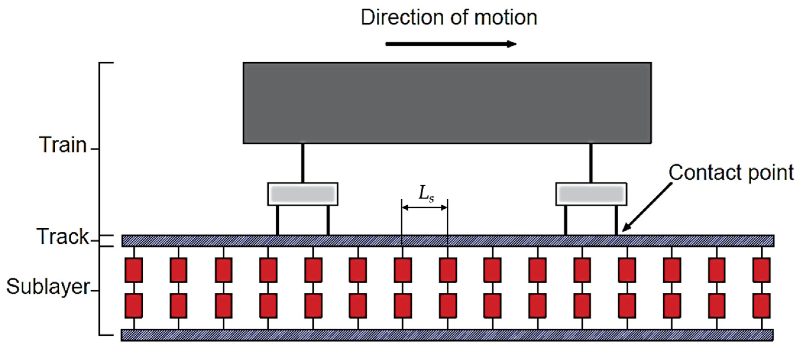
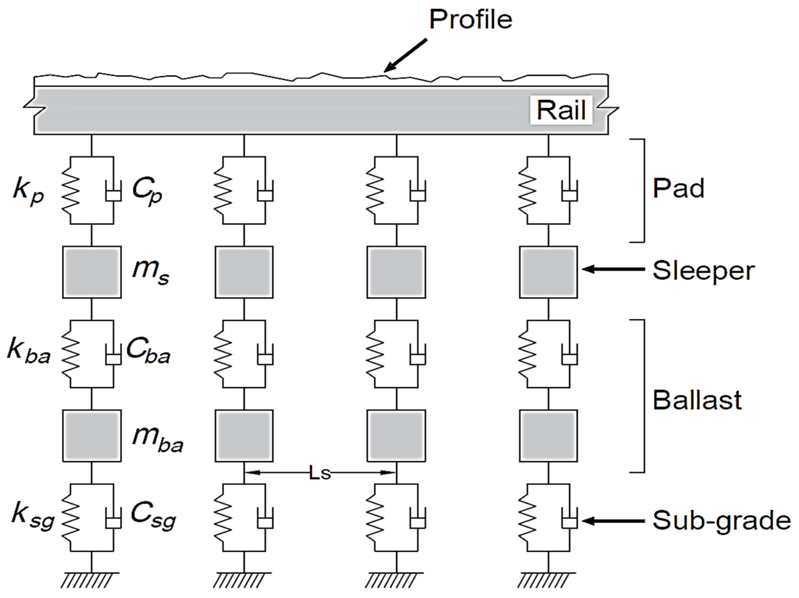
2.1. Track model
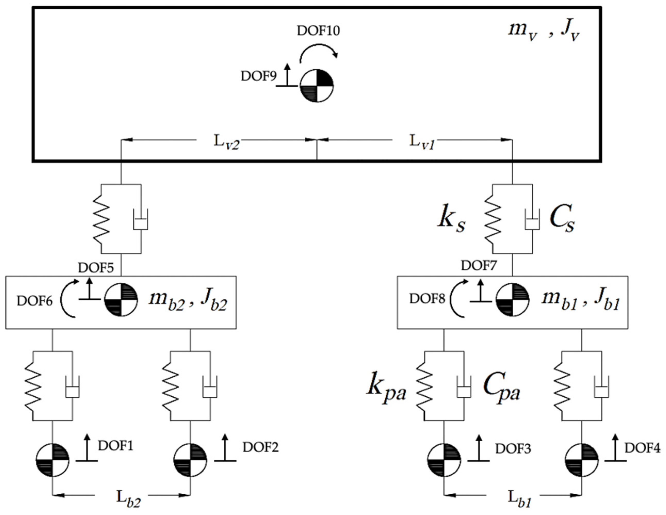
2.2. Train Model
2.3. Coupling of Train–Track Models
2.4. Modeling of Damage
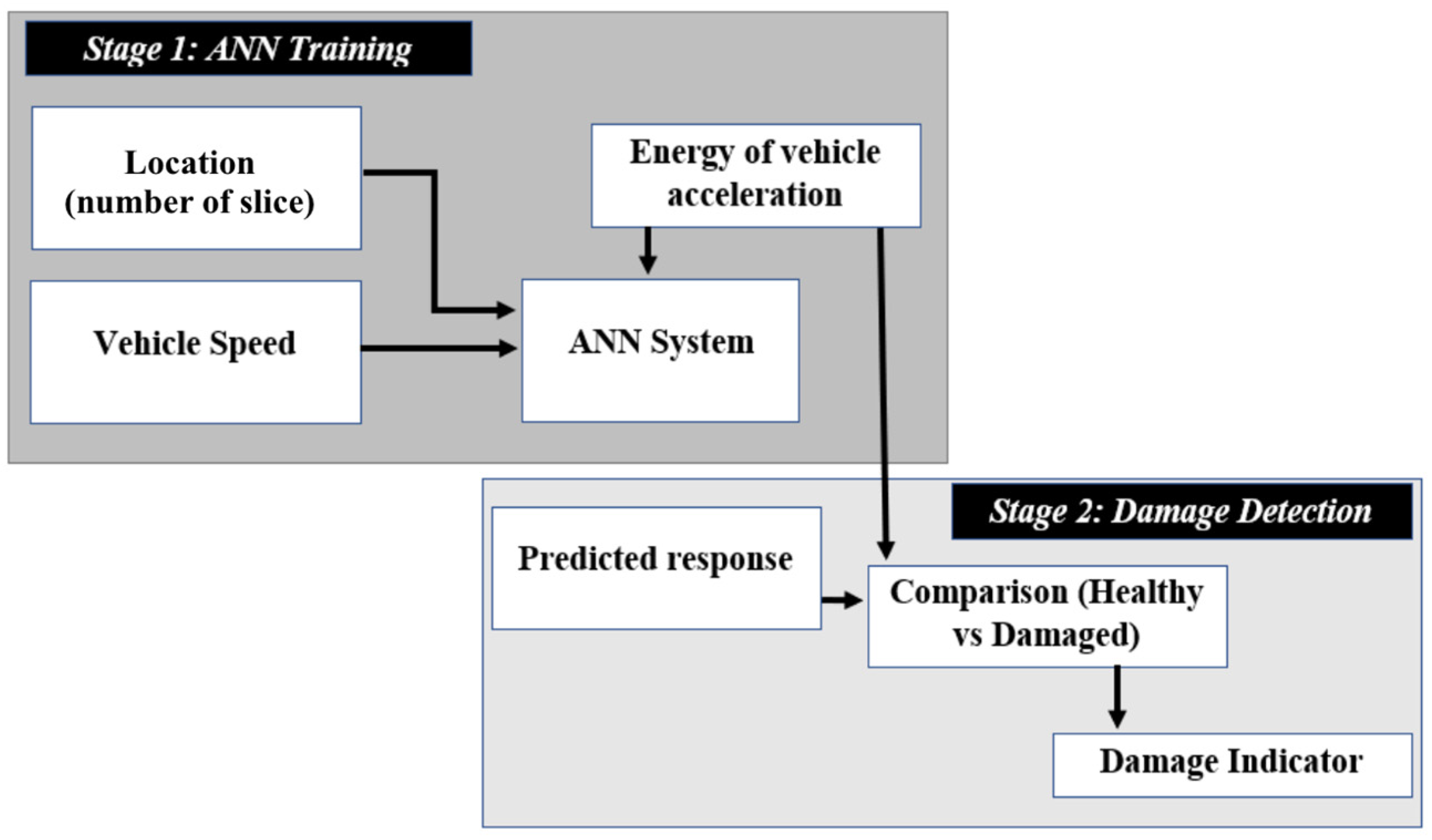
3. The Proposed Algorithm for Track Monitoring
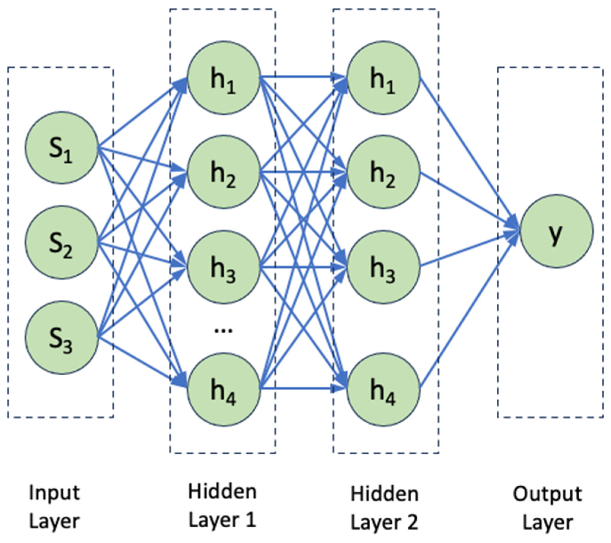
3.1. ANN Background
3.2. The Proposed ANN Model
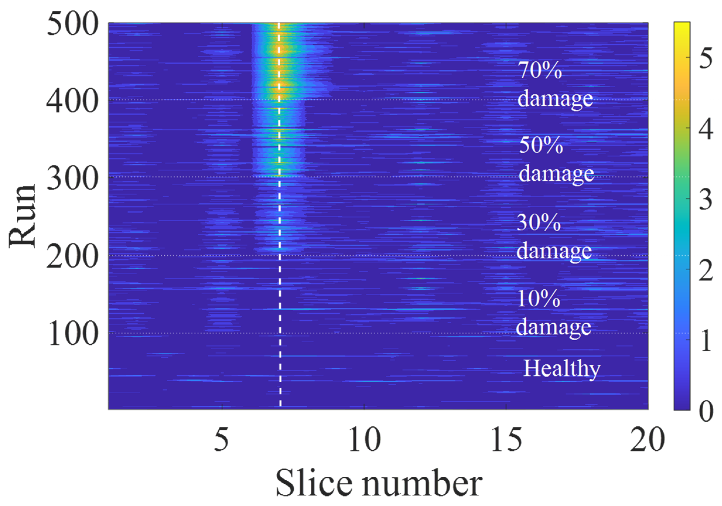
3.3. Damage Indicator
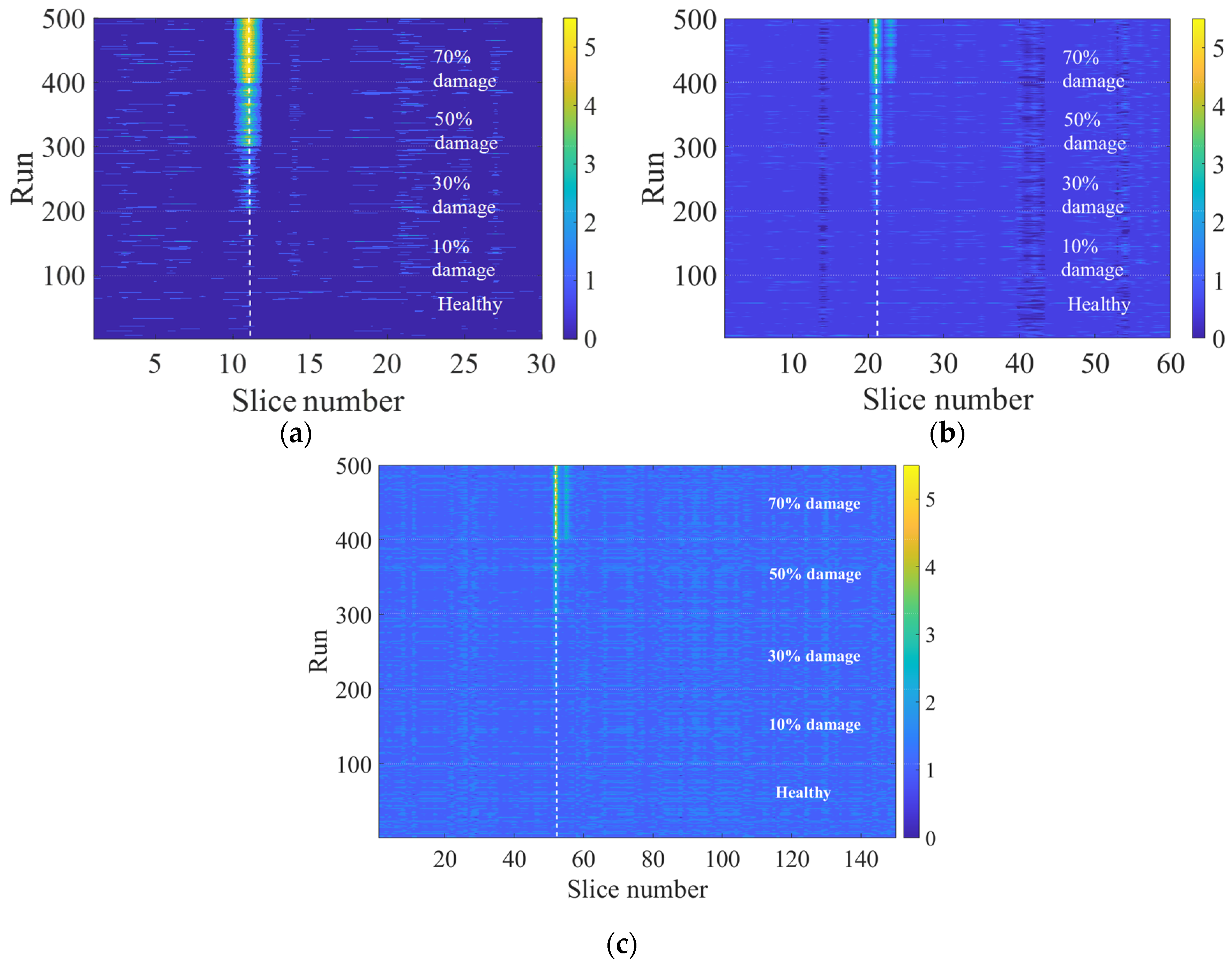
4. Result of the Machine Learning
5. Sensitivity Analysis
5.1. Size of Segments
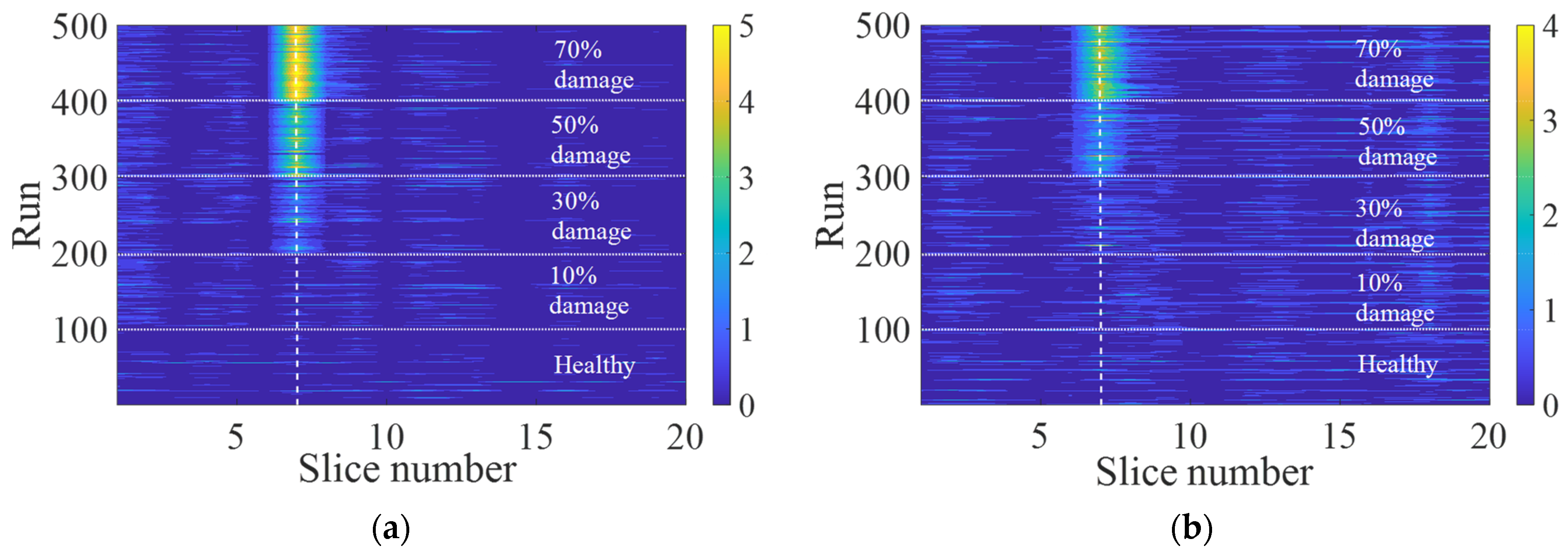
5.2. Noise Assessment
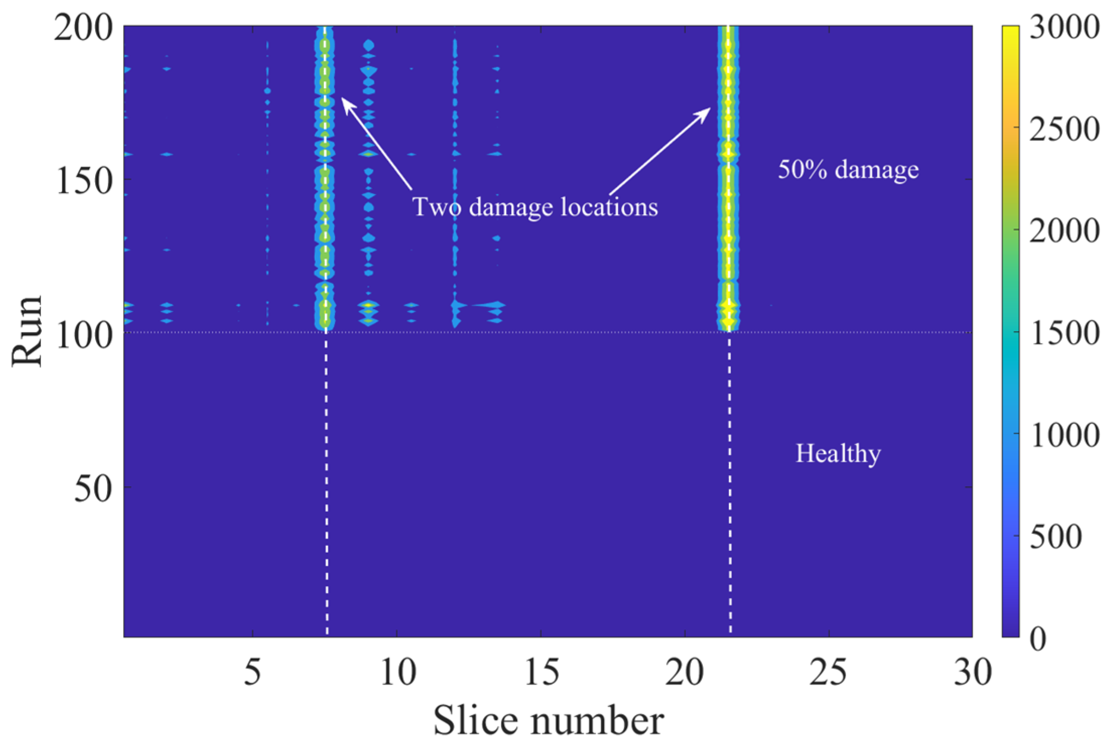
5.3. Multiple Damage Locations
6. Conclusions
Author Contributions
Funding
Institutional Review Board Statement
Informed Consent Statement
Data Availability Statement
Conflicts of Interest
References
- Schneider, A. Railway Safety Research–A Cross-Disciplinary Literature Review; Universität Koblenz, Universitätsbibliothek: Koblenz, Germany, 2020. [Google Scholar]
- Gao, N.; Touran, A. Cost overruns and formal risk assessment program in US rail transit projects. J. Constr. Eng. Manag. 2020, 146, 05020004. [Google Scholar] [CrossRef]
- Malekjafarian, A.; Obrien, E.J.; Quirke, P.; Cantero, D.; Golpayegani, F. Railway Track Loss-of-Stiffness Detection Using Bogie Filtered Displacement Data Measured on a Passing Train. Infrastructures 2021, 6, 93. [Google Scholar] [CrossRef]
- Kaewunruen, S.; Remennikov, A.M. Field trials for dynamic characteristics of railway track and its components using impact excitation technique. NDT E Int. 2007, 40, 510–519. [Google Scholar] [CrossRef]
- Koks, E.E.; Rozenberg, J.; Zorn, C.; Tariverdi, M.; Vousdoukas, M.; Fraser, S.A.; Hall, J.W.; Hallegatte, S. A global multi-hazard risk analysis of road and railway infrastructure assets. Nat. Commun. 2019, 10, 2677. [Google Scholar] [CrossRef]
- Quirke, P.; Obrien, E.J.; Bowe, C.; Cantero, D.; Malekjafarian, A. The calibration challenge when inferring longitudinal track profile from the inertial response of an in-service train. Can. J. Civ. Eng. 2022, 49, 274–288. [Google Scholar] [CrossRef]
- Azim, M.R.; Gül, M. Damage detection of steel girder railway bridges utilizing operational vibration response. Struct. Control Health Monit. 2019, 26, e2447. [Google Scholar] [CrossRef]
- Rageh, A.; Azam, S.E.; Linzell, D.G. Steel railway bridge fatigue damage detection using numerical models and machine learning: Mitigating influence of modeling uncertainty. Int. J. Fatigue 2020, 134, 105458. [Google Scholar] [CrossRef]
- Barke, D.; Chiu, W.K. Structural Health Monitoring in the Railway Industry: A Review. Struct. Health Monit. 2005, 4, 81–93. [Google Scholar] [CrossRef]
- Malekjafarian, A.; OBrien, E.J.; Golpayegani, F. Indirect monitoring of critical transport infrastructure: Data analytics and signal processing. In Data Analytics for Smart Cities; CRC Press: Boca Raton, FL, USA, 2018; pp. 157–176. [Google Scholar]
- Berggren, E.G.; Nissen, A.; Paulsson, B.S. Track deflection and stiffness measurements from a track recording car. Proc. Inst. Mech. Eng. Part. F J. Rail Rapid Transit. 2014, 228, 570–580. [Google Scholar] [CrossRef]
- Andrade, A.R.; Teixeira, P.F. Unplanned-maintenance needs related to rail track geometry. In Proceedings of the Institution of Civil Engineers-Transport; Thomas Telford Ltd.: London, UK, 2014. [Google Scholar]
- Wei, Z.; Núñez, A.; Li, Z.; Dollevoet, R. Evaluating Degradation at Railway Crossings Using Axle Box Acceleration Measurements. Sensors 2017, 17, 2236. [Google Scholar] [CrossRef]
- Chong, L.; Jiahong, W.; Zhixin, Z.; Junsheng, L.; Tongqun, R.; Hongquan, X. Design and evaluation of a remote measurement system for the online monitoring of rail vibration signals. Proc. Inst. Mech. Eng. Part. F J. Rail Rapid Transit. 2016, 230, 724–733. [Google Scholar] [CrossRef]
- Mennella, F.; Laudati, A.; Esposito, M.; Cusano, A.; Cutolo, A.; Giordano, M.; Campopiano, S.; Breglio, G. Railway monitoring and train tracking by fiber Bragg grating sensors. In Third European Workshop on Optical Fibre Sensors; International Society for Optics and Photonics: Bellingham, WA, USA, 2007. [Google Scholar]
- Kerrouche, A.; Boyle, W.; Gebremichael, Y.; Sun, T.; Grattan, K.; Täljsten, B.; Bennitz, A. Field tests of fibre Bragg grating sensors incorporated into CFRP for railway bridge strengthening condition monitoring. Sens. Actuators A Phys. 2008, 148, 68–74. [Google Scholar] [CrossRef]
- Fitzgerald, P.C.; Malekjafarian, A.; Cantero, D.; Obrien, E.J.; Prendergast, L.J. Drive-by scour monitoring of railway bridges using a wavelet-based approach. Eng. Struct. 2019, 191, 1–11. [Google Scholar] [CrossRef]
- Bocciolone, M.; Caprioli, A.; Cigada, A.; Collina, A. A measurement system for quick rail inspection and effective track maintenance strategy. Mech. Syst. Signal Process. 2007, 21, 1242–1254. [Google Scholar] [CrossRef]
- Molodova, M.; Li, Z.; Dollevoet, R. Axle box acceleration: Measurement and simulation for detection of short track defects. Wear 2011, 271, 349–356. [Google Scholar] [CrossRef]
- Lederman, G.; Chen, S.; Garrett, J.; Kovačević, J.; Noh, H.Y.; Bielak, J. Track-monitoring from the dynamic response of an operational train. Mech. Syst. Signal Process. 2017, 87, 1–16. [Google Scholar] [CrossRef]
- Bowe, C.; Quirke, P.; Cantero, D.; OBrien, E.J. Drive-by structural health monitoring of railway bridges using train mounted accelerometers. In Proceedings of the 5th ECCOMAS Thematic Conference on Computational Methods in Structural Dynamics and Earthquake Engineering, Crete Island, Greece, 25–27 May 2015. [Google Scholar]
- Nafari, S.F.; Gül, M.; Roghani, A.; Hendry, M.T.; Cheng, J.R. Evaluating the potential of a rolling deflection measurement system to estimate track modulus. Proc. Inst. Mech. Eng. Part. F J. Rail Rapid Transit. 2018, 232, 14–24. [Google Scholar] [CrossRef]
- Bar-Am, M. On-Train Rail Track Monitoring System. U.S. Patent 8942426B2, 27 January 2015. [Google Scholar]
- Fosburgh, B.A.; Nichols, M.E.; Holmgren, P.M.; Larsson, N.T. Railway Track Monitoring. U.S. Patent 9810533B2, 7 November 2017. [Google Scholar]
- Obrien, E.J.; Quirke, P.; Bowe, C.; Cantero, D. Determination of railway track longitudinal profile using measured inertial response of an in-service railway vehicle. Struct. Health Monit. 2018, 17, 1425–1440. [Google Scholar] [CrossRef]
- Malekjafarian, A.; Obrien, E.; Quirke, P.; Bowe, C. Railway Track Monitoring Using Train Measurements: An Experimental Case Study. Appl. Sci. 2019, 9, 4859. [Google Scholar] [CrossRef]
- Zhai, W.; Han, Z.; Chen, Z.; Ling, L.; Zhu, S. Train–track–bridge dynamic interaction: A state-of-the-art review. Veh. Syst. Dyn. 2019, 57, 984–1027. [Google Scholar] [CrossRef]
- Obrien, E.J.; Bowe, C.; Quirke, P.; Cantero, D. Determination of longitudinal profile of railway track using vehicle-based inertial readings. Proc. Inst. Mech. Eng. Part. F J. Rail Rapid Transit. 2017, 231, 518–534. [Google Scholar] [CrossRef]
- Wahlbin, L.B.; Bathe, K.-J.; Wilson, E.L. Numerical Methods in Finite Element Analysis; Prentice-Hall: Hoboken, NJ, USA, 1976. [Google Scholar]
- Avci, O.; Abdeljaber, O.; Kiranyaz, S.; Hussein, M.; Gabbouj, M.; Inman, D.J. A review of vibration-based damage detection in civil structures: From traditional methods to Machine Learning and Deep Learning applications. Mech. Syst. Signal Process. 2021, 147, 107077. [Google Scholar] [CrossRef]
- Malekjafarian, A.; Golpayegani, F.; Moloney, C.; Clarke, S. A Machine Learning Approach to Bridge-Damage Detection Using Responses Measured on a Passing Vehicle. Sensors 2019, 19, 4035. [Google Scholar] [CrossRef] [PubMed]
- Peng, J.; Zhang, S.; Peng, D.; Liang, K. Application of machine learning method in bridge health monitoring. In Proceedings of the 2017 Second International Conference on Reliability Systems Engineering (ICRSE), Beijing, China, 10–12 July 2017. [Google Scholar]
- Neves, A.C.; González, I.; Leander, J.; Karoumi, R. Structural health monitoring of bridges: A model-free ANN-based approach to damage detection. J. Civ. Struct. Health Monit. 2017, 7, 689–702. [Google Scholar] [CrossRef]
- Gonzalez, I.; Karoumi, R. BWIM aided damage detection in bridges using machine learning. J. Civ. Struct. Health Monit. 2015, 5, 715–725. [Google Scholar] [CrossRef]
- Santos, A.; Figueiredo, E.; Silva, M.; Santos, R.; Sales, C.; Costa, J.C.W.A. Genetic-based EM algorithm to improve the robustness of Gaussian mixture models for damage detection in bridges. Struct. Control Health Monit. 2017, 24, e1886. [Google Scholar] [CrossRef]
- Corbally, R.; Malekjafarian, A. A data-driven approach for drive-by damage detection in bridges considering the influence of temperature change. Eng. Struct. 2022, 253, 113783. [Google Scholar] [CrossRef]
- Diez, A.; Khoa, N.L.D.; Alamdari, M.M.; Wang, Y.; Chen, F.; Runcie, P. A clustering approach for structural health monitoring on bridges. J. Civ. Struct. Health Monit. 2016, 6, 429–445. [Google Scholar] [CrossRef]
- Goi, Y.; Kim, C.-W. Damage detection of a truss bridge utilizing a damage indicator from multivariate autoregressive model. J. Civ. Struct. Health Monit. 2017, 7, 153–162. [Google Scholar] [CrossRef]
- Khodabandehlou, H.; Pekcan, G.; Fadali, M.S. Vibration-based structural condition assessment using convolution neural networks. Struct. Control Health Monit. 2019, 26, e2308. [Google Scholar] [CrossRef]
- Kordestani, H.; Zhang, C.; Shadabfar, M. Beam Damage Detection Under a Moving Load Using Random Decrement Technique and Savitzky–Golay Filter. Sensors 2019, 20, 243. [Google Scholar] [CrossRef]
- Malekjafarian, A.; Moloney, C.; Golpayegani, F. Drive-by bridge health monitoring using multiple passes and machine learning. In European Workshop on Structural Health Monitoring; Springer: Berlin/Heidelberg, Germany, 2020. [Google Scholar]
- Kaewunruen, S.; Sresakoolchai, J.; Zhu, G. Machine learning aided rail corrugation monitoring for railway track maintenance. Struct. Monit. Maint. 2021, 8, 151–166. [Google Scholar]
- Sresakoolchai, J.; Kaewunruen, S. Wheel flat detection and severity classification using deep learning techniques. Insight—Non-Destr. Test. Cond. Monit. 2021, 63, 393–402. [Google Scholar] [CrossRef]
- Quirke, P.; Obrien, E.J.; Bowe, C.; Malekjafarian, A.; Cantero, D. Estimation of railway track longitudinal profile using vehicle-based inertial measurements. In Sustainable Solutions for Railways and Transportation Engineering, Proceedings of the International Congress and Exhibition “Sustainable Civil Infrastructures: Innovative Infrastructure Geotechnology”, Cairo, Egypt, 24–28 November 2018; Springer: Berlin/Heidelberg, Germany, 2018. [Google Scholar]
- Cantero, D.; O’Brien, E.J.; González, A. Modelling the vehicle in vehicle—Infrastructure dynamic interaction studies. Proc. Inst. Mech. Eng. Part. K J. Multi-Body Dyn. 2010, 224, 243–248. [Google Scholar] [CrossRef]
- Cantero, D. VEqMon2D—Equations of motion generation tool of 2D vehicles with Matlab. SoftwareX 2022, 19, 101103. [Google Scholar] [CrossRef]
- Cantero, D.; Arvidsson, T.; OBrien, E.; Karoumi, R. Train–track–bridge modelling and review of parameters. Struct. Infrastruct. Eng. 2016, 12, 1051–1064. [Google Scholar] [CrossRef]
- Zhai, W.; Wang, K.; Cai, C. Fundamentals of vehicle–track coupled dynamics. Veh. Syst. Dyn. 2009, 47, 1349–1376. [Google Scholar] [CrossRef]
- Nguyen, K.; Goicolea, J.; Galbadón, F. Comparison of dynamic effects of high-speed traffic load on ballasted track using a simplified two-dimensional and full three-dimensional model. Proc. Inst. Mech. Eng. Part. F J. Rail Rapid Transit. 2014, 228, 128–142. [Google Scholar] [CrossRef]
- Zhai, W.; Wang, K.; Lin, J. Modelling and experiment of railway ballast vibrations. J. Sound. Vib. 2004, 270, 673–683. [Google Scholar] [CrossRef]
- Quirke, P.; Cantero, D.; Obrien, E.J.; Bowe, C. Drive-by detection of railway track stiffness variation using in-service vehicles. Proc. Inst. Mech. Eng. Part. F J. Rail Rapid Transit. 2017, 231, 498–514. [Google Scholar] [CrossRef]
- Lei, X.; Noda, N.-A. Analyses of dynamic response of vehicle and track coupling system with random irregularity of track vertical profile. J. Sound. Vib. 2002, 258, 147–165. [Google Scholar] [CrossRef]
- Kwon, Y.W.; Bang, H. The Finite Element Method Using MATLAB; CRC Press: Boca Raton, FL, USA, 2018. [Google Scholar]
- González, A. Vehicle-bridge dynamic interaction using finite element modelling. In Finite Element Analysis; Moratal, D., Ed.; InTechOpen: Rijeka, Croatia, 2010; pp. 637–662. [Google Scholar]
- Kaynia, A.M.; Park, J.; Norén-Cosgriff, K. Effect of track defects on vibration from high speed train. Procedia Eng. 2017, 199, 2681–2686. [Google Scholar] [CrossRef]
- Jin, C.; Jang, S.; Sun, X.; Li, J.; Christenson, R. Damage detection of a highway bridge under severe temperature changes using extended Kalman filter trained neural network. J. Civ. Struct. Health Monit. 2016, 6, 545–560. [Google Scholar] [CrossRef]
- Cavadas, F.; Smith, I.F.; Figueiras, J. Damage detection using data-driven methods applied to moving-load responses. Mech. Syst. Signal Process. 2013, 39, 409–425. [Google Scholar] [CrossRef]
- Sapna, S.; Tamilarasi, A.; Kumar, M.P. Backpropagation learning algorithm based on Levenberg Marquardt Algorithm. Comp. Sci. Inform. Technol. (CS IT) 2012, 2, 393–398. [Google Scholar]
- Yu, H.; Wilamowski, B.M. Levenberg-marquardt training. In Industrial Electronics Handbook; CRC Press: Boca Raton, FL, USA, 2011; Volume 5, p. 1. [Google Scholar]
- Keenahan, J.; Obrien, E.J.; McGetrick, P.J.; Gonzalez, A. The use of a dynamic truck–trailer drive-by system to monitor bridge damping. Struct. Health Monit. 2014, 13, 143–157. [Google Scholar] [CrossRef]
- Khan, M.A.; McCrum, D.P.; Prendergast, L.J.; Obrien, E.J.; Fitzgerald, P.C.; Kim, C.-W. Laboratory investigation of a bridge scour monitoring method using decentralized modal analysis. Struct. Health Monit. 2021, 20, 3327–3341. [Google Scholar] [CrossRef]


| Property | Unit | Value |
|---|---|---|
| Elastic modulus of rail | N/m2 | 2.059 × 10¹¹ |
| Rail cross-sectional area | m2 | 1 |
| Rail second moment of area | m4 | 3.217 × 10⁻⁵ |
| Rail mass per unit length | kg/m | 60.64 |
| Rail pad stiffness | N/m | 6.5 × 10⁷ |
| Rail pad damping | Ns/m | 7.5 × 10⁴ |
| Sleeper mass (half) | kg | 125.5 |
| Sleeper spacing | m | 0.545 |
| Ballast stiffness | N/m | 137.75 × 10⁶ |
| Ballast damping | Ns/m | 5.88 × 10⁴ |
| Ballast mass | kg | 531.4 |
| Subgrade stiffness mean | N/m | 77.5 × 10⁶ |
| Subgrade damping | Ns/m | 3.115 × 10⁴ |
| Property | Symbol | Unit | Value |
|---|---|---|---|
| Wheelset mass | mw | kg | 1843.5 |
| Bogie mass | mb | kg | 59,364.2 |
| Car body mass | mv | kg | 5630.8 |
| Moment of inertia of bogie | Jb | kg·m2 | 9487 |
| Moment of inertia of main body | Jv | kg·m2 | 1.723 × 10⁶ |
| Primary suspension stiffness | kpa | N/m | 2.399 × 10⁶ |
| Secondary suspension stiffness | ks | N/m | 0.8858 × 10⁶ |
| Primary suspension damping | cpa | Ns/m | 30 × 103 |
| Secondary suspension damping | Cs | Ns/m | 45 × 103 |
| Distance between car body center of mass and bogie pivot | Lv1, Lv2 | m | 5.73 |
| Distance between axles | Lb1, Lb2 | m | 3 |
Disclaimer/Publisher’s Note: The statements, opinions and data contained in all publications are solely those of the individual author(s) and contributor(s) and not of MDPI and/or the editor(s). MDPI and/or the editor(s) disclaim responsibility for any injury to people or property resulting from any ideas, methods, instructions or products referred to in the content. |
© 2023 by the authors. Licensee MDPI, Basel, Switzerland. This article is an open access article distributed under the terms and conditions of the Creative Commons Attribution (CC BY) license (https://creativecommons.org/licenses/by/4.0/).
Share and Cite
Malekjafarian, A.; Sarrabezolles, C.-A.; Khan, M.A.; Golpayegani, F. A Machine-Learning-Based Approach for Railway Track Monitoring Using Acceleration Measured on an In-Service Train. Sensors 2023, 23, 7568. https://doi.org/10.3390/s23177568
Malekjafarian A, Sarrabezolles C-A, Khan MA, Golpayegani F. A Machine-Learning-Based Approach for Railway Track Monitoring Using Acceleration Measured on an In-Service Train. Sensors. 2023; 23(17):7568. https://doi.org/10.3390/s23177568
Chicago/Turabian StyleMalekjafarian, Abdollah, Chalres-Antoine Sarrabezolles, Muhammad Arslan Khan, and Fatemeh Golpayegani. 2023. "A Machine-Learning-Based Approach for Railway Track Monitoring Using Acceleration Measured on an In-Service Train" Sensors 23, no. 17: 7568. https://doi.org/10.3390/s23177568