
Shot Boundary Detection with 3D Depthwise Convolutions and Visual Attention

 , and
, and
Abstract
:1. Introduction
- 1.
- 2.
- The usage of a residual self-attention block with attention map computation and the verification of the performance of the models.
- 3.
- We provide comparative results, testing the performance of the models in three different sets of experiments. A first set with no depthwise convolutions, a second set with only depthwise convolutions, and a third set where we combine depthwise convolutions and residual attention blocks.
2. Related Work
3. Motivation and High-Level Considerations
4. Proposed Methods
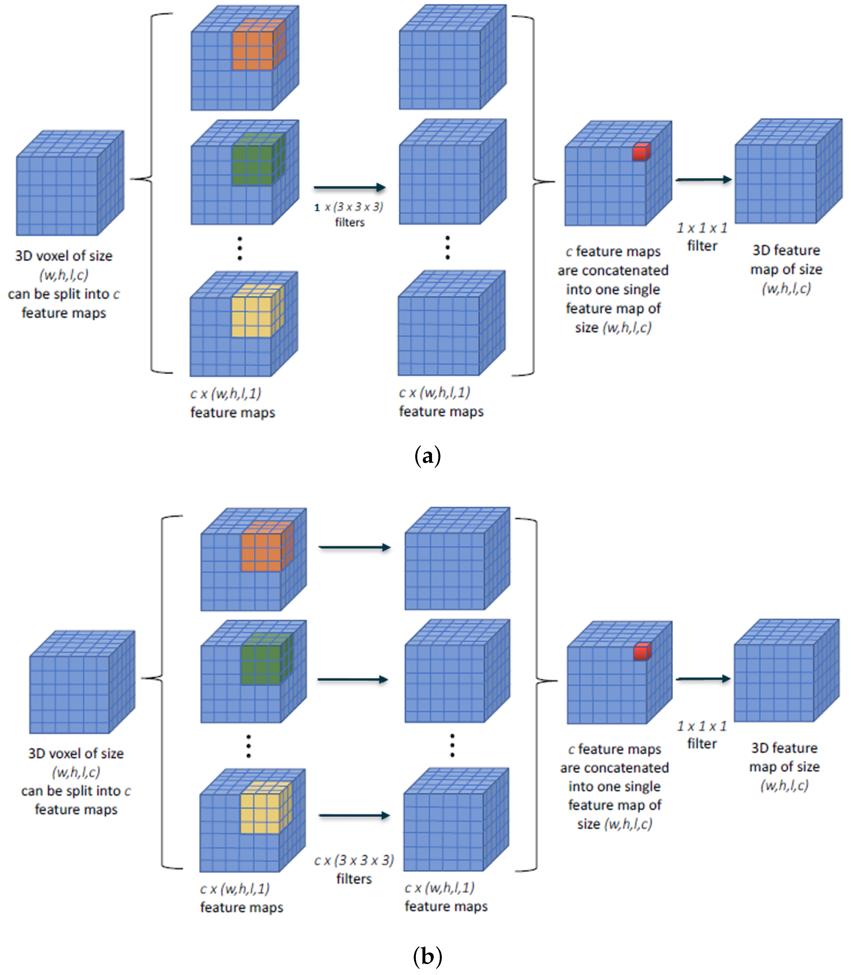
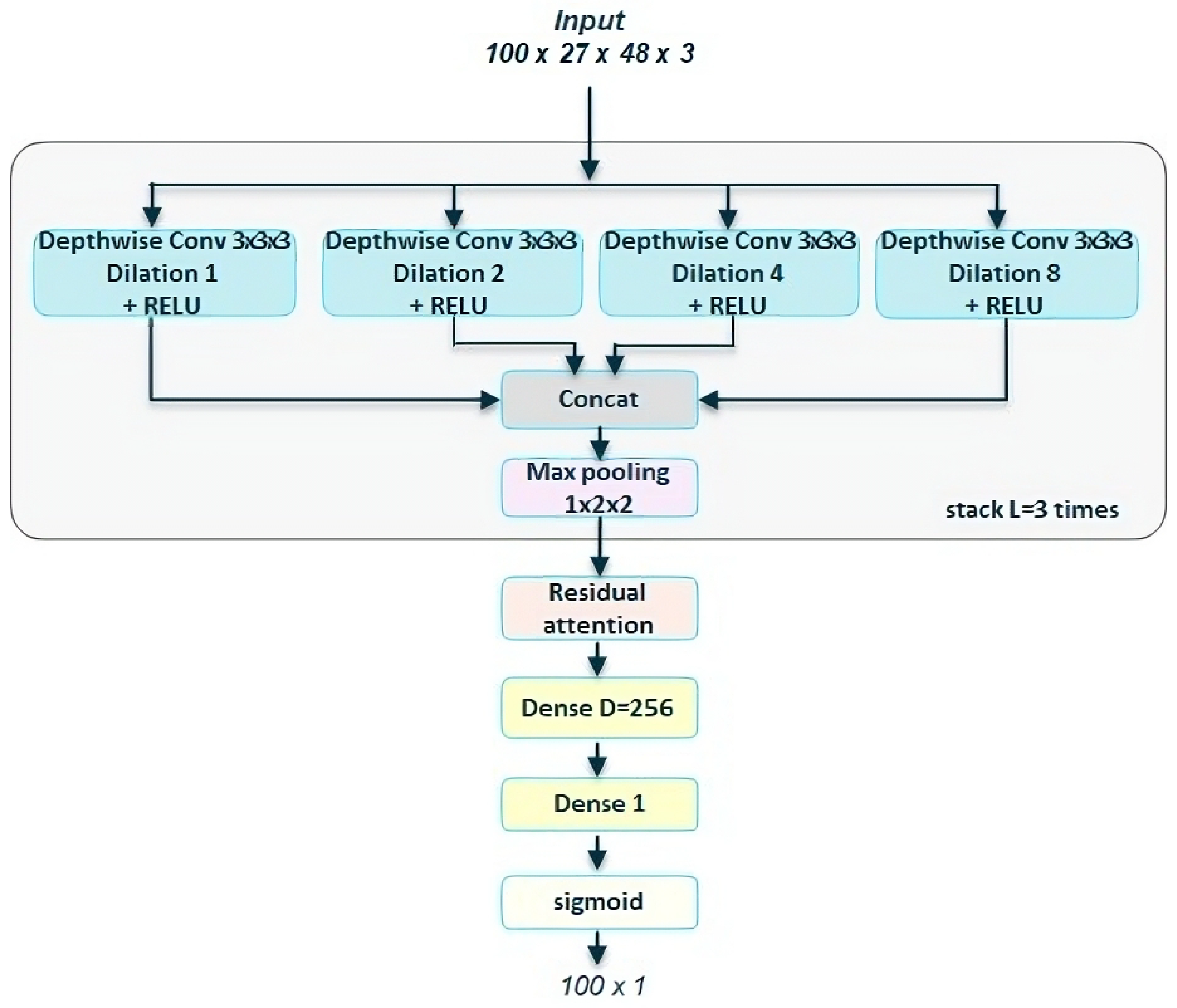
4.1. Depthwise Separable Convolution
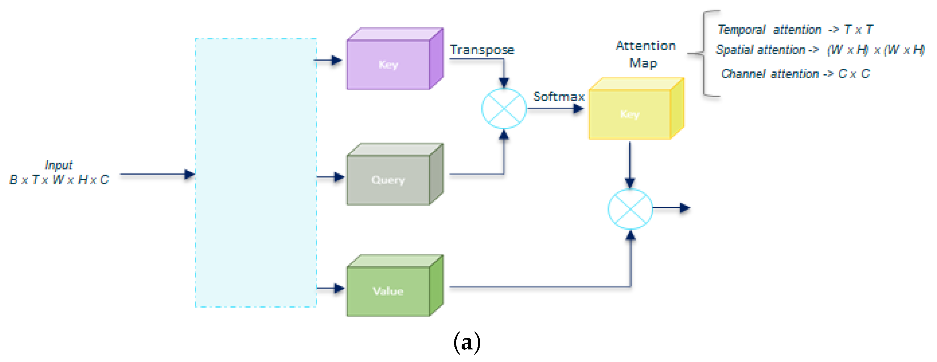
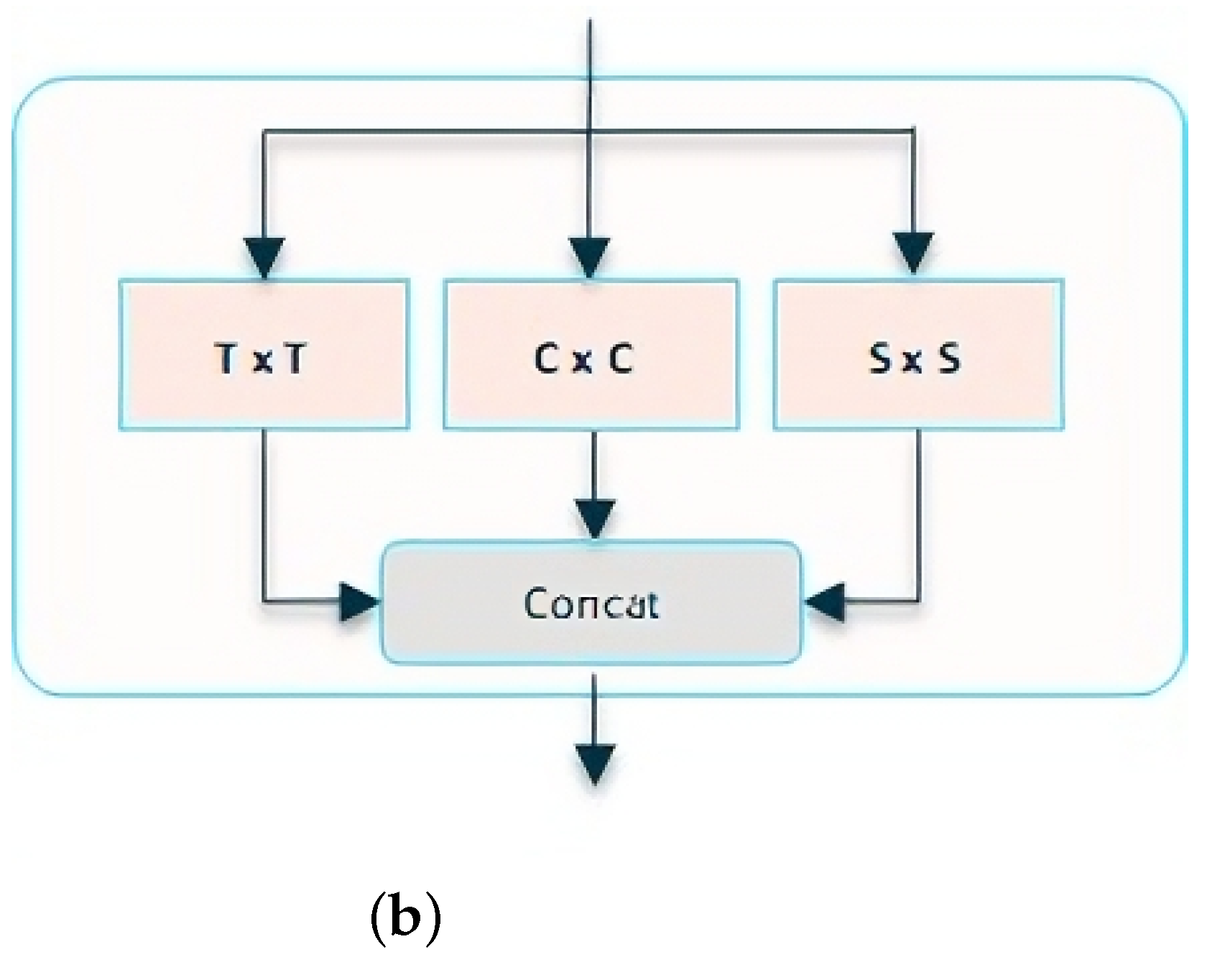
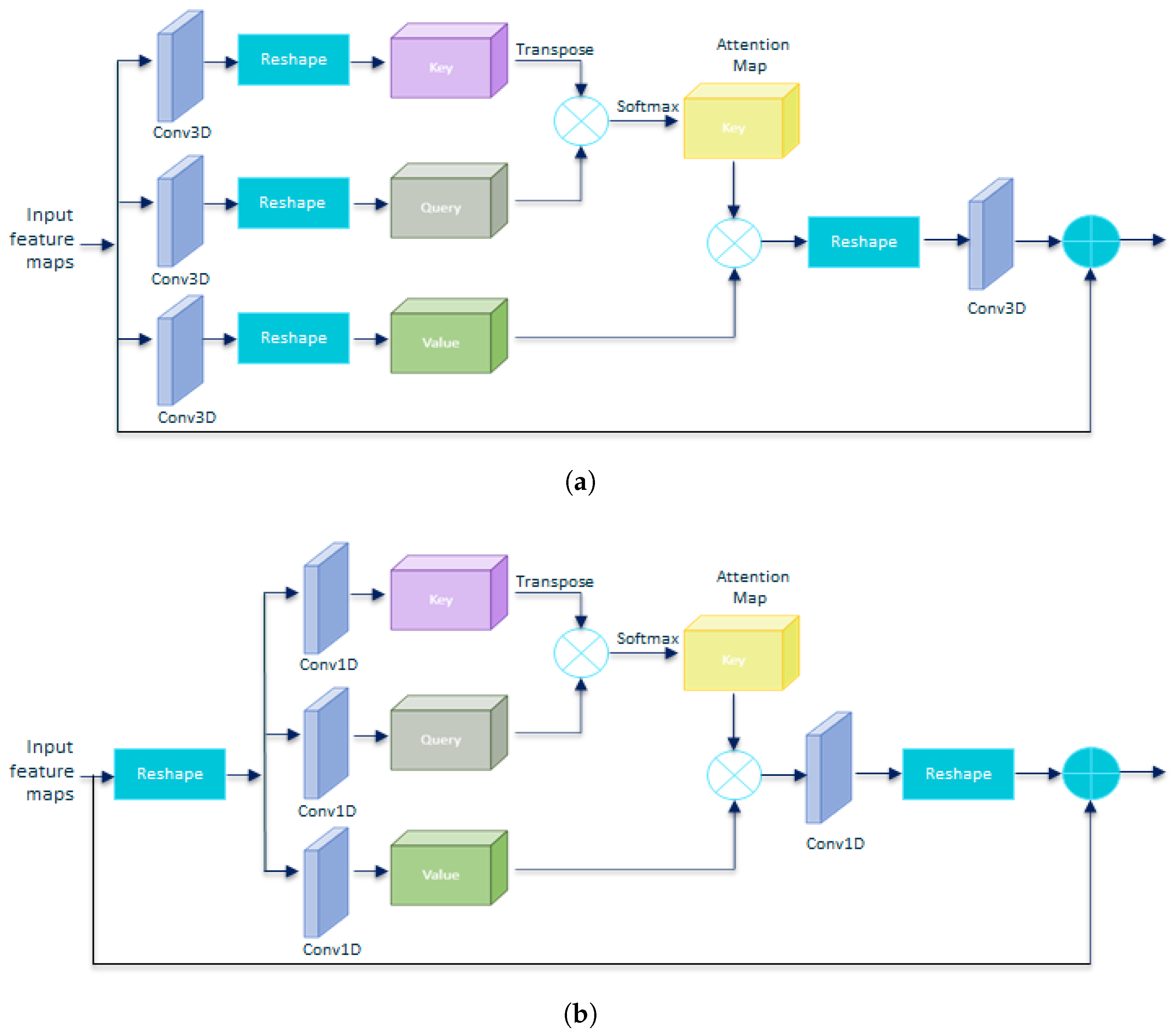
4.2. Residual Self-Attention
4.3. Architectural Options
4.3.1. Type of Depthwise Convolution
4.3.2. Attention Blocks on a Different Axis
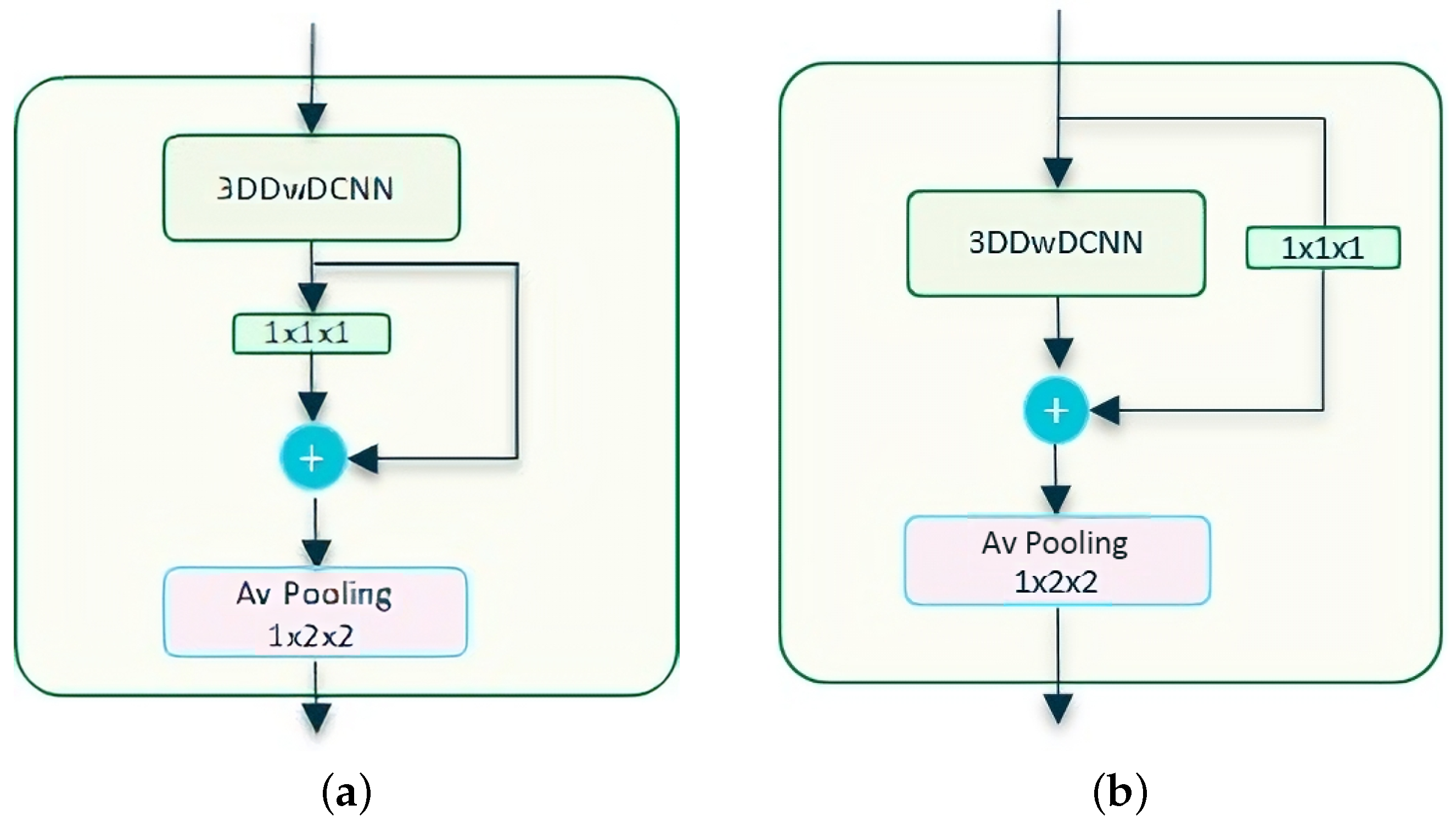
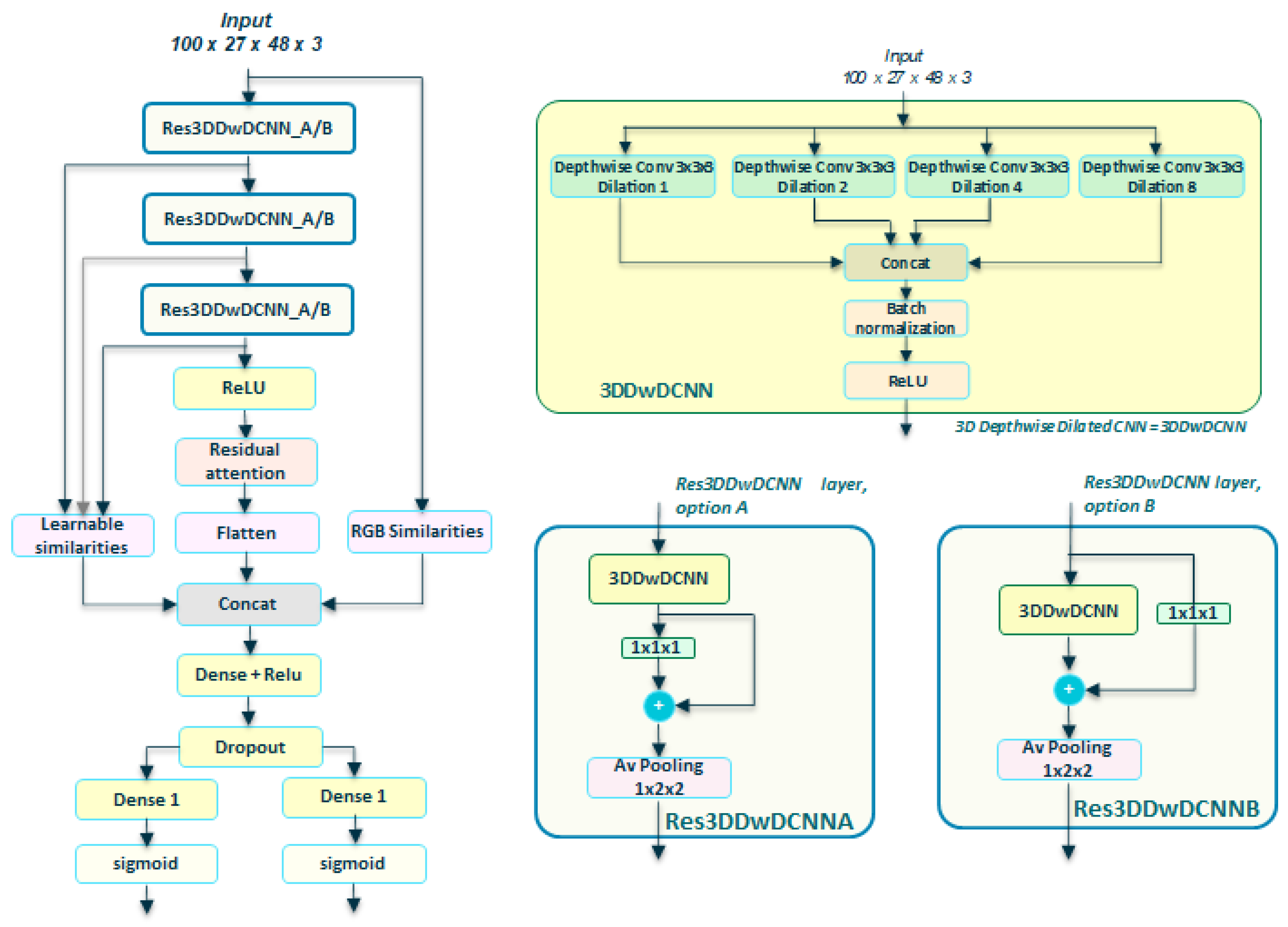
4.3.3. Residual Depthwise Dilated options
4.3.4. Residual Self-Attention Options
4.4. Final Modified Networks
- where:
- –
- X refers to the depthwise option. X = 1 for one shared convolution for all channels option. X = 2 for the one different convolution for each channel option.
- –
- Type refers to the Attention type, with , and T: temporal, S: spatial (WxH), C: channel, M: multiple.
- –
- Z refers to attention convolutions. Z = 1 for Conv3D; Z = 2 for Conv1D
- –
- Y, with Y = A for ResDw3DCNN option A, and Y = A for ResDw3DCNN option B. This option only applies for Transnetv2.
4.5. Networks Parameters
5. Experiments
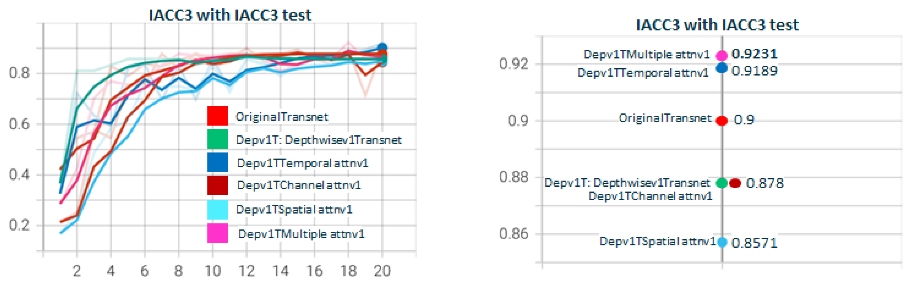
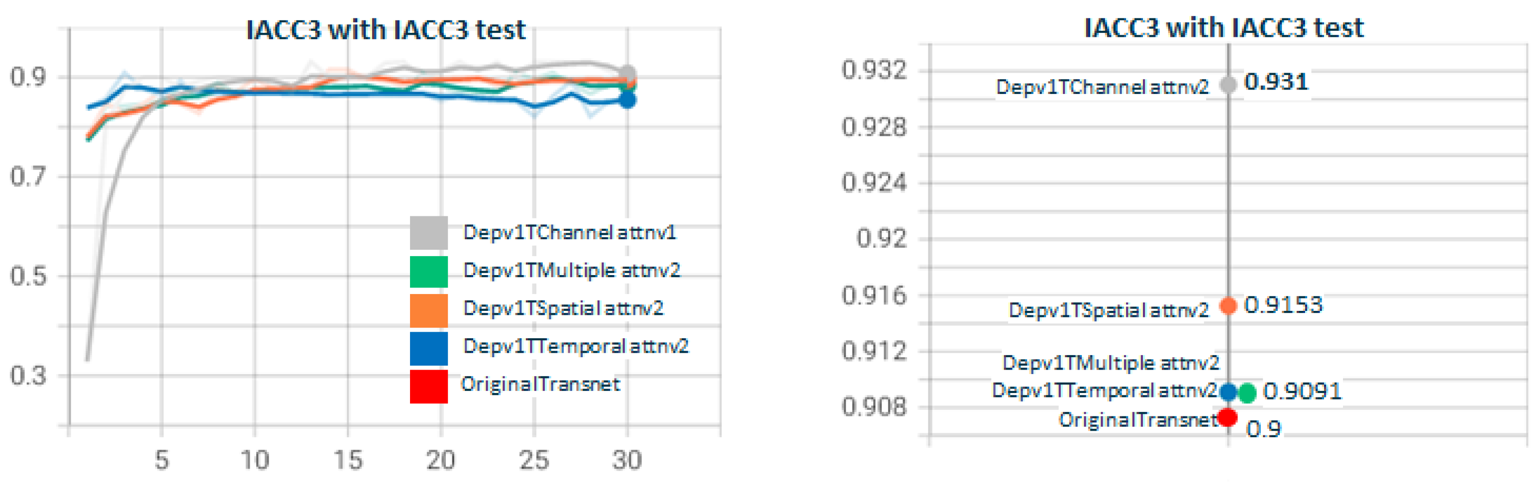
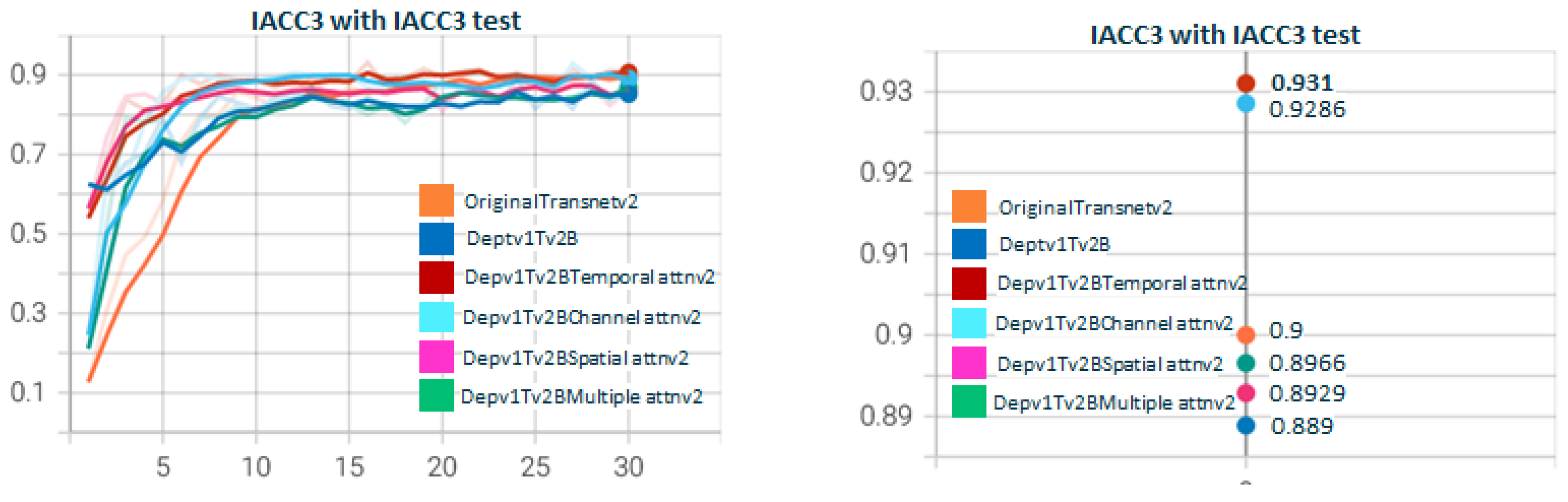
5.1. Depthwisev{X}TransnetAttn{Type}v{Z} Experiments
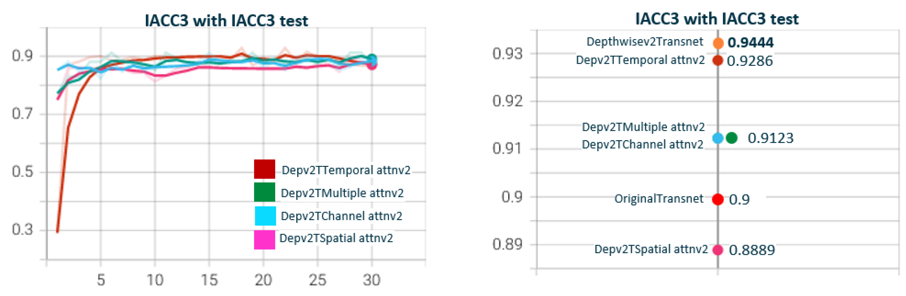
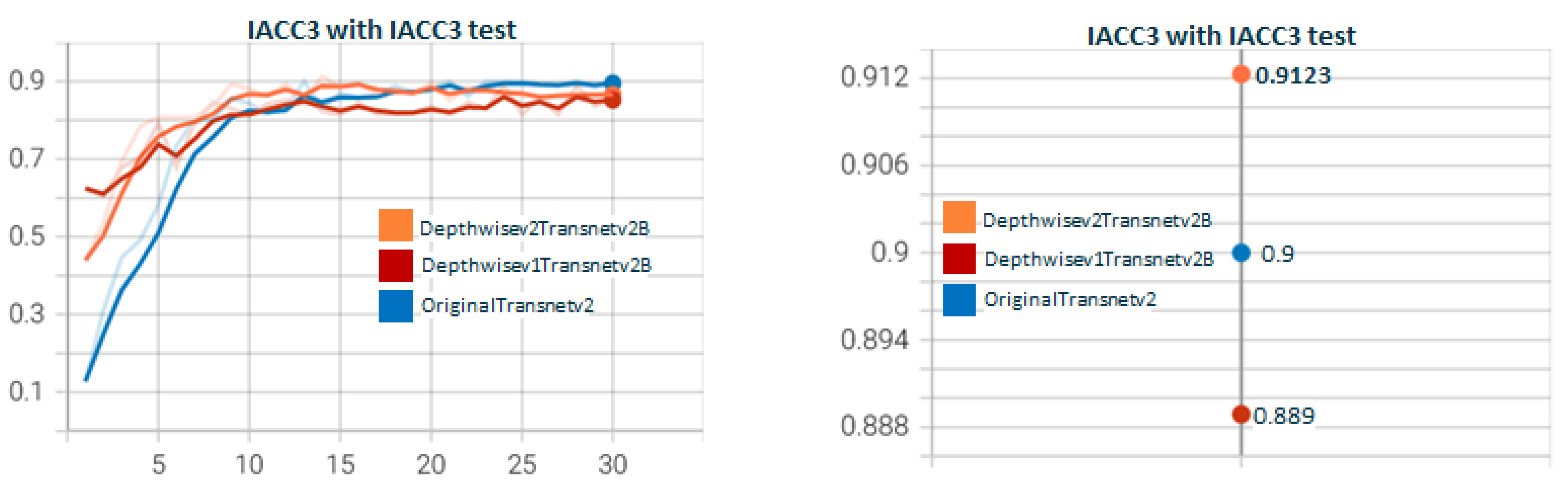
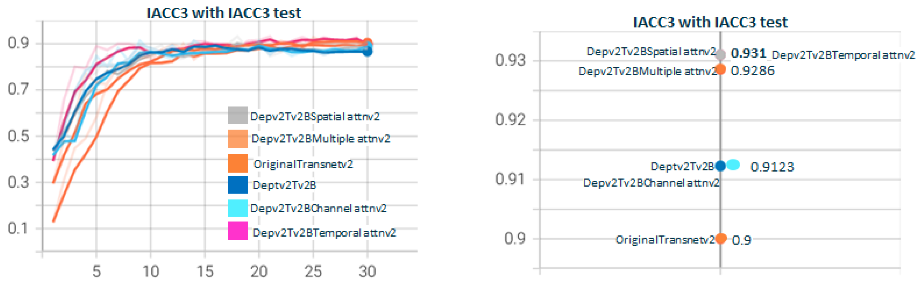
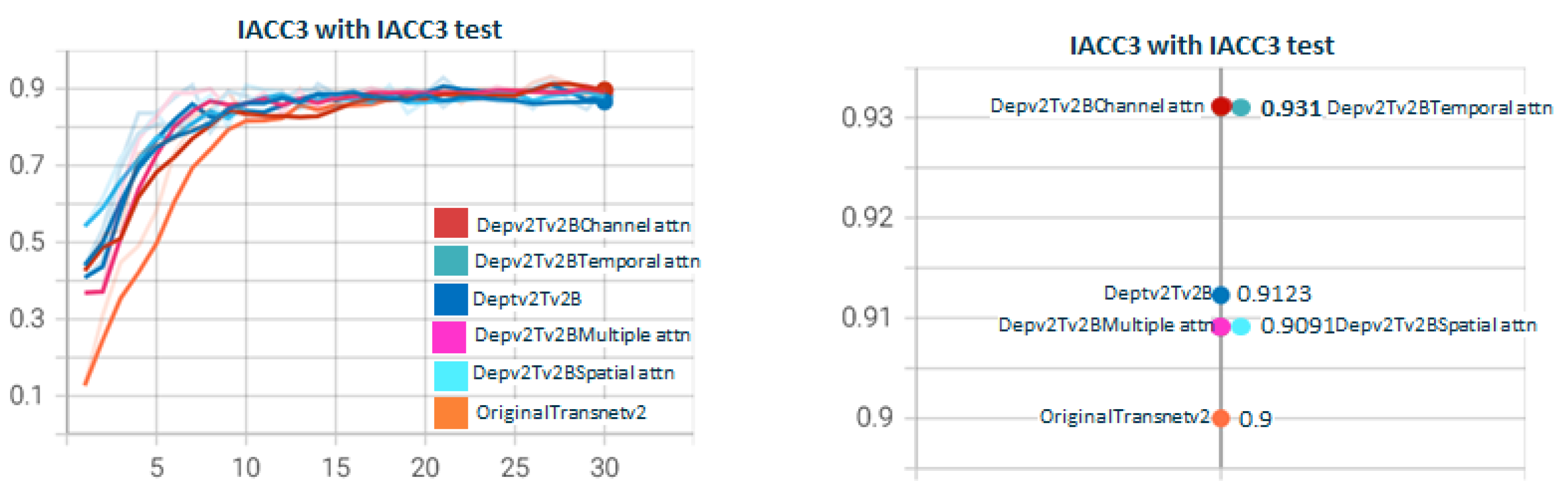
5.2. Depthwisev{X}Transnetv2{Y}Attn{Type}v{Z} Experiments
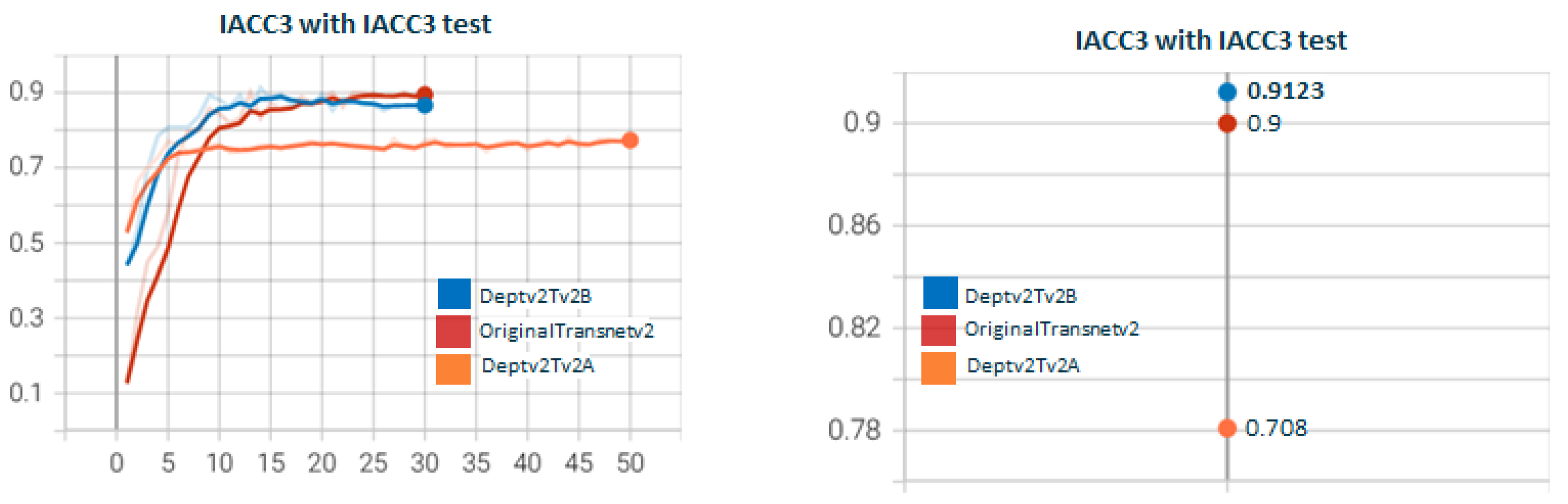
5.3. Other Experiments
6. Conclusions
Author Contributions
Funding
Data Availability Statement
Acknowledgments
Conflicts of Interest
References
- Howard, A.G.; Zhu, M.; Chen, B.; Kalenichenko, D.; Wang, W.; Weyand, T.; Andreetto, M.; Adam, H. MobileNets: Efficient Convolutional Neural Networks for Mobile Vision Applications. arXiv 2017, arXiv:1704.04861. [Google Scholar]
- Chollet, F. Xception: Deep Learning with Depthwise Separable Convolutions. arXiv 2017, arXiv:1610.02357. [Google Scholar]
- Hu, J.; Shen, L.; Albanie, S.; Sun, G.; Wu, E. Squeeze-and-Excitation Networks. arXiv 2019, arXiv:1709.01507. [Google Scholar]
- Li, X.; Wang, W.; Hu, X.; Yang, J. Selective Kernel Networks. arXiv 2019, arXiv:1903.06586. [Google Scholar]
- Souček, T.; Moravec, J.; Lokoč, J. TransNet: A deep network for fast detection of common shot transitions. arXiv 2019, arXiv:1906.03363v1. [Google Scholar] [CrossRef]
- Souček, T.; Lokoč, J. TransNet V2: An effective deep network architecture for fast shot transition detection. arXiv 2020, arXiv:2008.04838. [Google Scholar] [CrossRef]
- Jin, J.; Dundar, A.; Culurciello, E. Flattened Convolutional Neural Networks for Feedforward Acceleration. arXiv 2015, arXiv:1412.5474. [Google Scholar]
- Wang, M.; Liu, B.; Foroosh, H. Factorized Convolutional Neural Networks. In Proceedings of the 2017 IEEE International Conference on Computer Vision Workshops (ICCVW), Venice, Italy, 22–29 October 2017; pp. 545–553. [Google Scholar] [CrossRef]
- Liu, B.; Wang, M.; Foroosh, H.; Tappen, M.; Penksy, M. Sparse Convolutional Neural Networks. In Proceedings of the 2015 IEEE Conference on Computer Vision and Pattern Recognition (CVPR), Boston, MA, USA, 7–12 June 2015; pp. 806–814. [Google Scholar] [CrossRef]
- Szegedy, C.; Vanhoucke, V.; Ioffe, S.; Shlens, J.; Wojna, Z. Rethinking the Inception Architecture for Computer Vision. arXiv 2015, arXiv:1512.00567. [Google Scholar]
- Szegedy, C.; Ioffe, S.; Vanhoucke, V.; Alemi, A. Inception-v4, Inception-ResNet and the Impact of Residual Connections on Learning. arXiv 2016, arXiv:1602.07261. [Google Scholar] [CrossRef]
- He, K.; Zhang, X.; Ren, S.; Sun, J. Deep Residual Learning for Image Recognition. arXiv 2015, arXiv:1512.03385. [Google Scholar]
- Carreira, J.; Zisserman, A. Quo Vadis, Action Recognition? A New Model and the Kinetics Dataset. arXiv 2018, arXiv:1705.07750. [Google Scholar]
- Donahue, J.; Hendricks, L.A.; Rohrbach, M.; Venugopalan, S.; Guadarrama, S.; Saenko, K.; Darrell, T. Long-term Recurrent Convolutional Networks for Visual Recognition and Description. arXiv 2016, arXiv:1411.4389. [Google Scholar]
- Ng, J.Y.H.; Hausknecht, M.; Vijayanarasimhan, S.; Vinyals, O.; Monga, R.; Toderici, G. Beyond Short Snippets: Deep Networks for Video Classification. arXiv 2015, arXiv:1503.08909. [Google Scholar]
- Feichtenhofer, C.; Pinz, A.; Zisserman, A. Convolutional Two-Stream Network Fusion for Video Action Recognition. arXiv 2016, arXiv:1604.06573. [Google Scholar]
- Simonyan, K.; Zisserman, A. Two-Stream Convolutional Networks for Action Recognition in Videos. arXiv 2014, arXiv:1406.2199. [Google Scholar]
- Tran, D.; Bourdev, L.; Fergus, R.; Torresani, L.; Paluri, M. Learning Spatiotemporal Features with 3D Convolutional Networks. arXiv 2015, arXiv:1412.0767. [Google Scholar]
- Xie, S.; Sun, C.; Huang, J.; Tu, Z.; Murphy, K. Rethinking Spatiotemporal Feature Learning: Speed-Accuracy Trade-offs in Video Classification. arXiv 2018, arXiv:1712.04851. [Google Scholar]
- Qiu, Z.; Yao, T.; Mei, T. Learning Spatio-Temporal Representation with Pseudo-3D Residual Networks. arXiv 2017, arXiv:1711.10305. [Google Scholar]
- Ye, R.; Liu, F.; Zhang, L. 3D Depthwise Convolution: Reducing Model Parameters in 3D Vision Tasks. arXiv 2018, arXiv:1808.01556. [Google Scholar]
- Zhang, X.; Zhou, X.; Lin, M.; Sun, J. ShuffleNet: An Extremely Efficient Convolutional Neural Network for Mobile Devices. arXiv 2017, arXiv:1707.01083. [Google Scholar]
- Sandler, M.; Howard, A.; Zhu, M.; Zhmoginov, A.; Chen, L.C. MobileNetV2: Inverted Residuals and Linear Bottlenecks. arXiv 2019, arXiv:1801.04381. [Google Scholar]
- Iandola, F.N.; Han, S.; Moskewicz, M.W.; Ashraf, K.; Dally, W.J.; Keutzer, K. SqueezeNet: AlexNet-level accuracy with 50x fewer parameters and <0.5MB model size. arXiv 2016, arXiv:1602.07360. [Google Scholar]
- Awad, G.; Butt, A.A.; Fiscus, J.G.; Joy, D.; Delgado, A.; Michel, M.; Smeaton, A.F.; Graham, Y.; Jones, G.J.; Kraaij, W.; et al. TRECVID 2017: Evaluating Ad-hoc and Instance Video Search, Events Detection, Video Captioning and Hyperlinking. In Proceedings of the TREC Video Retrieval Evaluation, Gaithersburg, MD, USA, 13–15 November 2017. [Google Scholar]
- Baraldi, L.; Grana, C.; Cucchiara, R. A Deep Siamese Network for Scene Detection in Broadcast Videos. In Proceedings of the 23rd ACM international conference on Multimedia, Brisbane, Australia, 26–30 October 2015; Association for Computing Machinery: New York, NY, USA, 2015. [Google Scholar] [CrossRef] [Green Version]
- Vaswani, A.; Shazeer, N.; Parmar, N.; Uszkoreit, J.; Jones, L.; Gomez, A.N.; Kaiser, L.; Polosukhin, I. Attention Is All You Need. In Proceedings of the Advances in Neural Information Processing Systems 30 (NIPS 2017), Long Beach, CA, USA, 4–9 December 2017. [Google Scholar]
- Zhang, H.; Goodfellow, I.; Metaxas, D.; Odena, A. Self-Attention Generative Adversarial Networks. In Proceedings of the 36th International Conference on Machine Learning, Long Beach, CA, USA, 9–15 June 2019. [Google Scholar]
- Fu, J.; Liu, J.; Tian, H.; Li, Y.; Bao, Y.; Fang, Z.; Lu, H. Dual Attention Network for Scene Segmentation. In Proceedings of the IEEE/CVF Conference on Computer Vision and Pattern Recognition (CVPR), Long Beach, CA, USA, 15–20 June 2019. [Google Scholar]
- Zhang, X.; Han, L.; Zhu, W.; Sun, L.; Zhang, D. An Explainable 3D Residual Self-Attention Deep Neural Network for Joint Atrophy Localization and Alzheimer’s Disease Diagnosis Using Structural MRI. IEEE J. Biomed. Health Inform. 2022, 26, 5289–5297. [Google Scholar] [CrossRef] [PubMed]
- Zhu, M.; Bin, S.; Sun, G. Lite-3DCNN Combined with Attention Mechanism for Complex Human Movement Recognition. Comput. Intell. Neurosci. 2022, 2022, 4816549. [Google Scholar] [CrossRef] [PubMed]
- Tang, S.; Feng, L.; Kuang, Z.; Chen, Y.; Zhang, W. Fast Video Shot Transition Localization with Deep Structured Models. In Asian Conference on Computer Vision; Springer: Cham, Switzerland, 2018. [Google Scholar] [CrossRef]
- Baraldi, L.; Grana, C.; Cucchiara, R. Shot and Scene Detection via Hierarchical Clustering for Re-using Broadcast Video. In Computer Analysis of Images and Patterns; Azzopardi, G., Petkov, N., Eds.; Springer: Cham, Switzerland, 2015; pp. 801–811. [Google Scholar]


| Depthwise | ||||
|---|---|---|---|---|
| Original | v1 | v2 | ||
| Transnet | 4.614.593 | 895.665 | 902.385 | |
| TransnetV2 | 4.763.970 | 1.060.526 | 1.067.246 | ResDw3DCNN_A |
| 1.031.042 | 1.037.762 | ResDw3DCNN_B | ||
| Depthwisev{X} | |||||||||
|---|---|---|---|---|---|---|---|---|---|
| X = 1 | X = 2 | ||||||||
| Attn{Type}v2 | Attn{Type}v2 | ||||||||
| T | C | S | M | T | C | S | M | ||
| Transnet: | 936.065 | 1.043.889 | 897.033 | 2.855.129 | 942.785 | 1.050.609 | 916.455 | 2.861.849 | |
| TransnetV2: | ResDw3DDCNN_A | 1.100.926 | 1.208.750 | 1.061.894 | 3.019.990 | 1.107.646 | 1.215.470 | 1.068.614 | 3.026.710 |
| ResDw3DDCNN_B | 1.1071.422 | 1.179.266 | 1.032.410 | 2.990.506 | 1.078.162 | 1.185.986 | 1.038.130 | 2.997.226 | |
| Dataset/Annotations | Original | Depthwisev2 | +Tempv2 | +Spav2 | +Chav2 | +Mulv2 |
|---|---|---|---|---|---|---|
| Transnet | 0.661 | 0.650 | 0.625 | 0.627 | 0.656 | 0.649 |
| TransnetV2 | 0.694 | 0.659 | 0.686 | 0.686 | 0.687 | 0.648 |
| Dataset/Annotations | Original | Depthwisev2 | +Tempv2 | +Spav2 | +Chav2 | +Mulv2 |
|---|---|---|---|---|---|---|
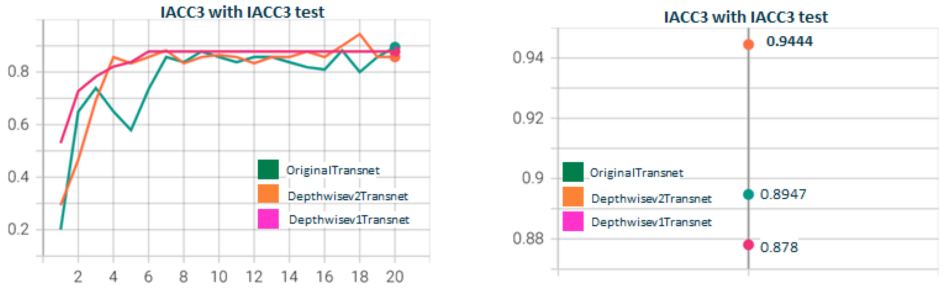
| Transnet | 0.931 | 0.921 | 0.930 | 0.912 | 0.925 | 0.944 |
| TransnetV2 | 0.916 | 0.927 | 0.920 | 0.916 | 0.922 | 0.913 |
| Dataset/Annotations | Original | Depthwisev2 | +Tempv2 | +Spav2 | +Chav2 | +Mulv2 |
|---|---|---|---|---|---|---|
| Transnet | 0.897 | 0.894 | 0.911 | 0.896 | 0.894 | 0.910 |
| TransnetV2 | 0.905 | 0.903 | 0.905 | 0.897 | 0.915 | 0.905 |
Disclaimer/Publisher’s Note: The statements, opinions and data contained in all publications are solely those of the individual author(s) and contributor(s) and not of MDPI and/or the editor(s). MDPI and/or the editor(s) disclaim responsibility for any injury to people or property resulting from any ideas, methods, instructions or products referred to in the content. |
© 2023 by the authors. Licensee MDPI, Basel, Switzerland. This article is an open access article distributed under the terms and conditions of the Creative Commons Attribution (CC BY) license (https://creativecommons.org/licenses/by/4.0/).
Share and Cite
Esteve Brotons, M.J.; Lucendo, F.J.; Javier, R.-J.; Garcia-Rodriguez, J. Shot Boundary Detection with 3D Depthwise Convolutions and Visual Attention. Sensors 2023, 23, 7022. https://doi.org/10.3390/s23167022
Esteve Brotons MJ, Lucendo FJ, Javier R-J, Garcia-Rodriguez J. Shot Boundary Detection with 3D Depthwise Convolutions and Visual Attention. Sensors. 2023; 23(16):7022. https://doi.org/10.3390/s23167022
Chicago/Turabian StyleEsteve Brotons, Miguel Jose, Francisco Javier Lucendo, Rodriguez-Juan Javier, and Jose Garcia-Rodriguez. 2023. "Shot Boundary Detection with 3D Depthwise Convolutions and Visual Attention" Sensors 23, no. 16: 7022. https://doi.org/10.3390/s23167022