
Design and Implementation of a Fuzzy Classifier for FDI Applied to Industrial Machinery


Abstract
:1. Introduction
2. Materials and Methods
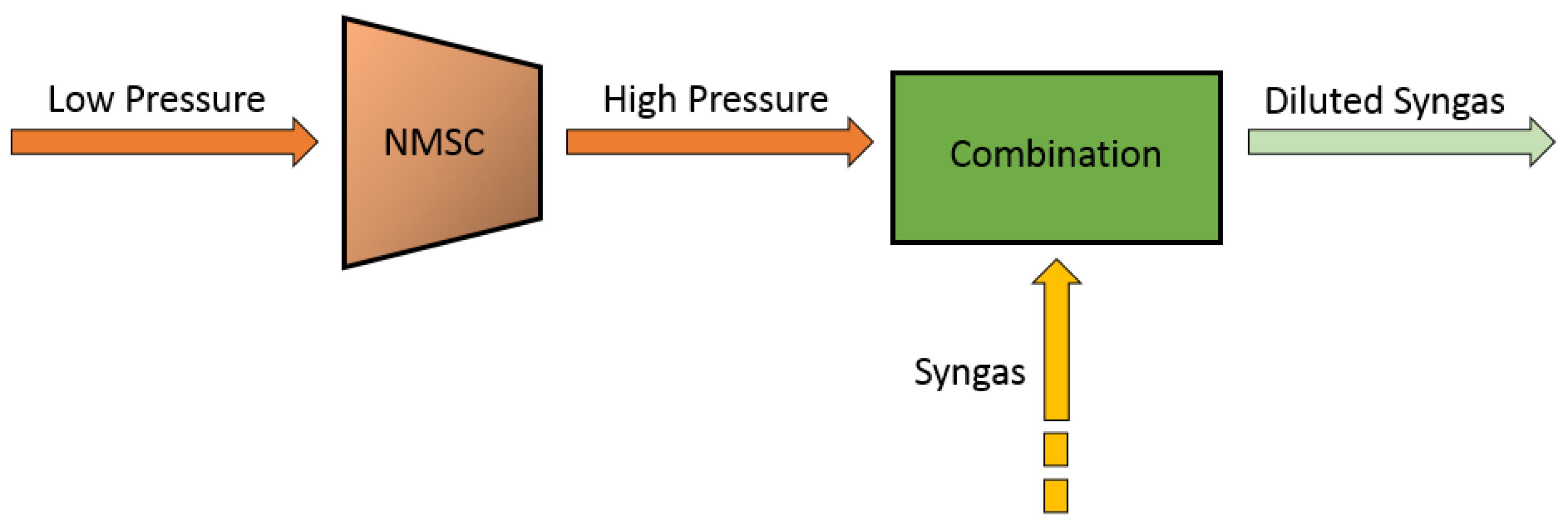
2.1. Plant Description
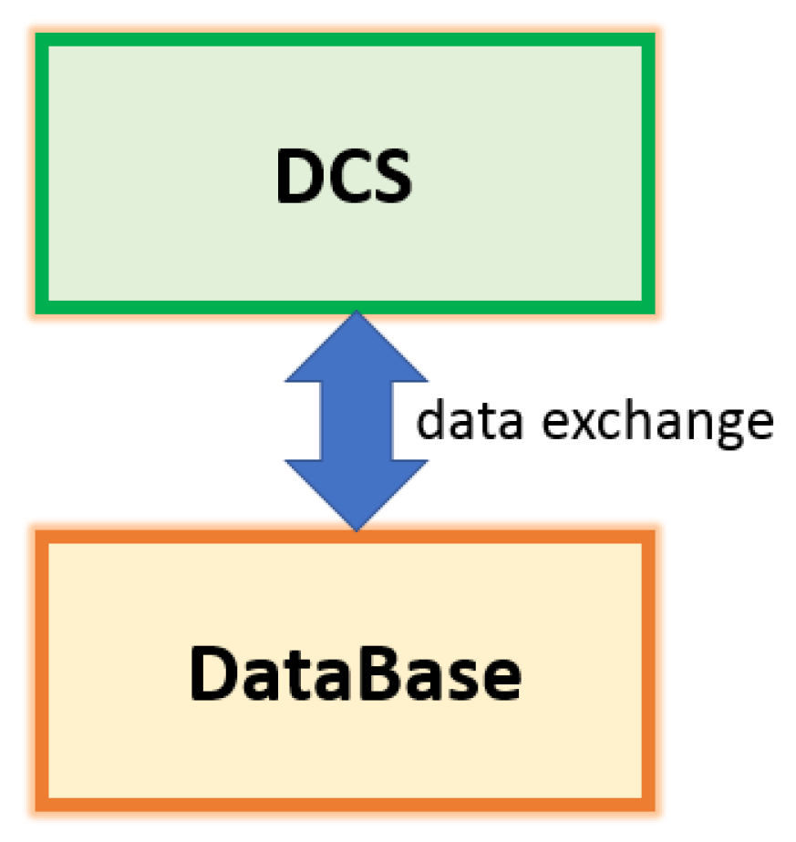
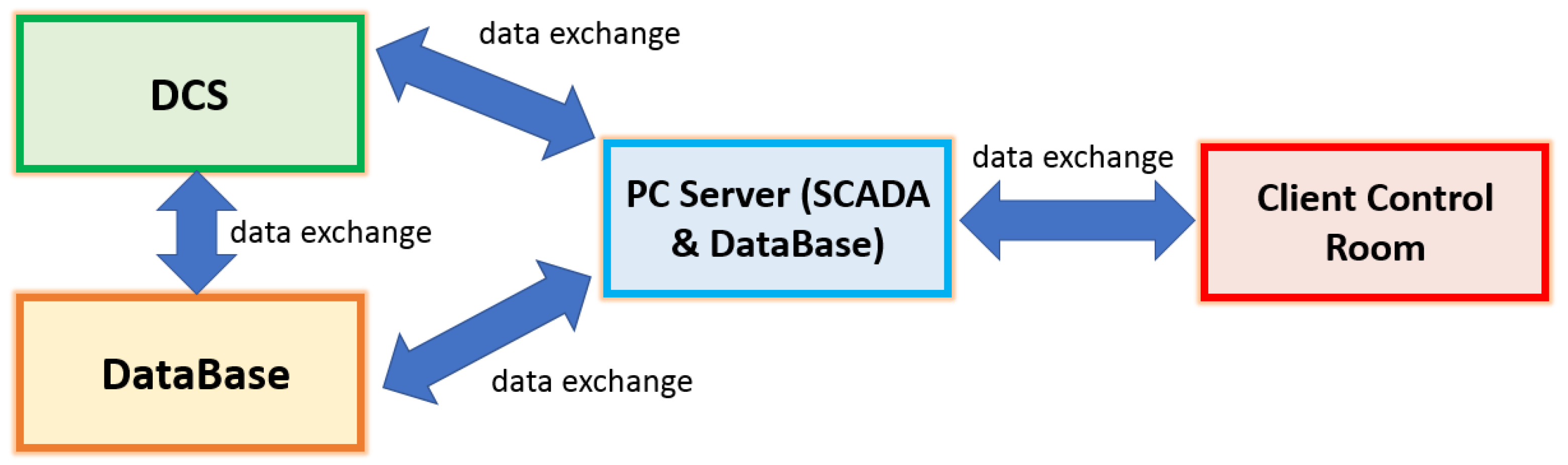
The Need of an FDI System on NMSC
2.2. Background on the PCA
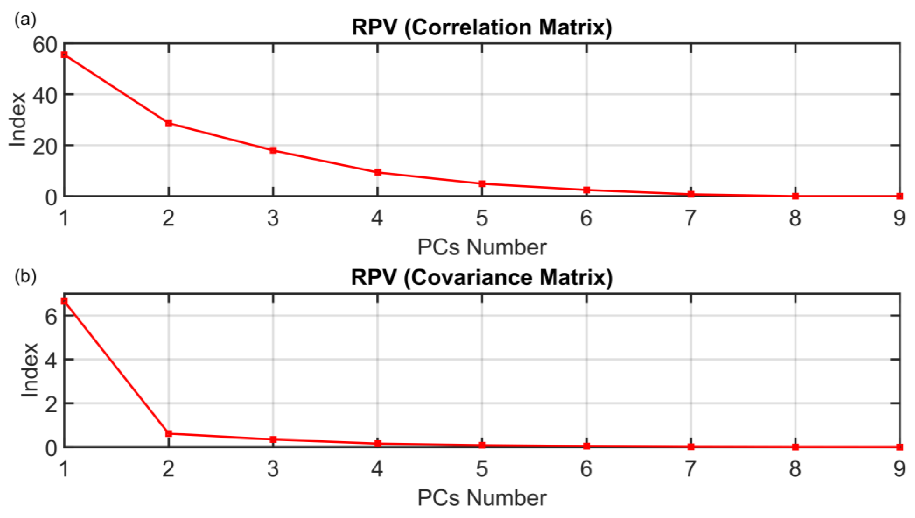
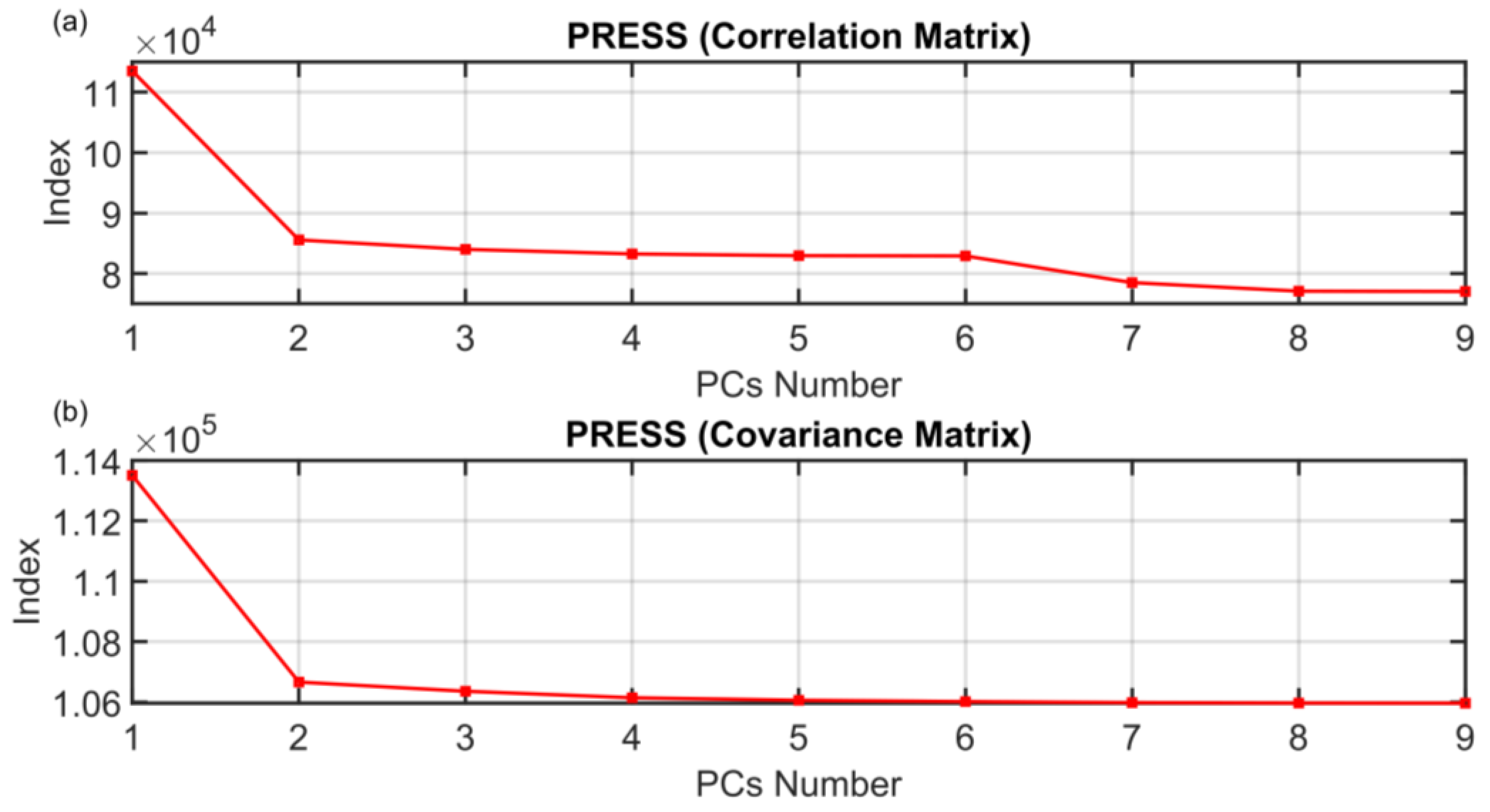
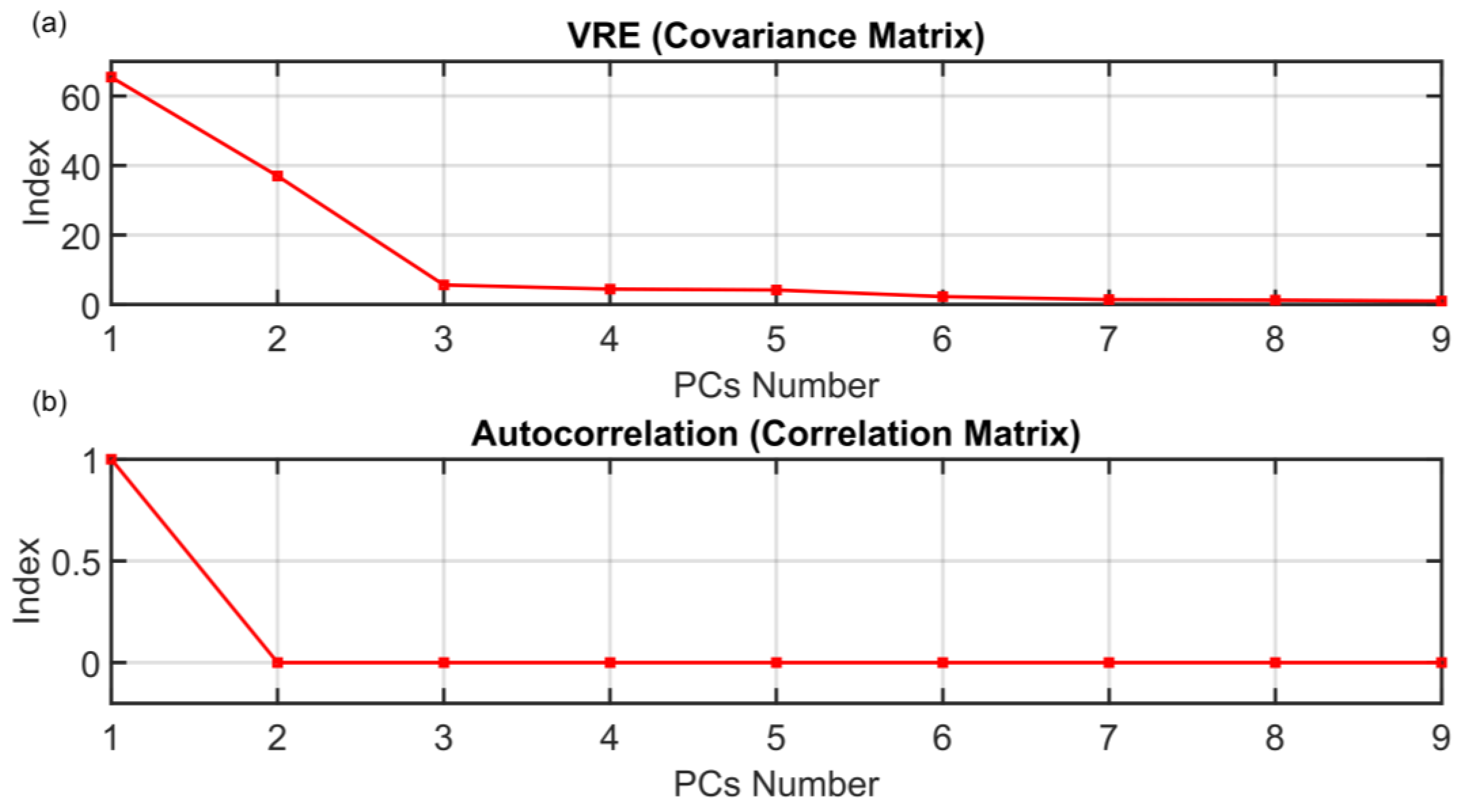
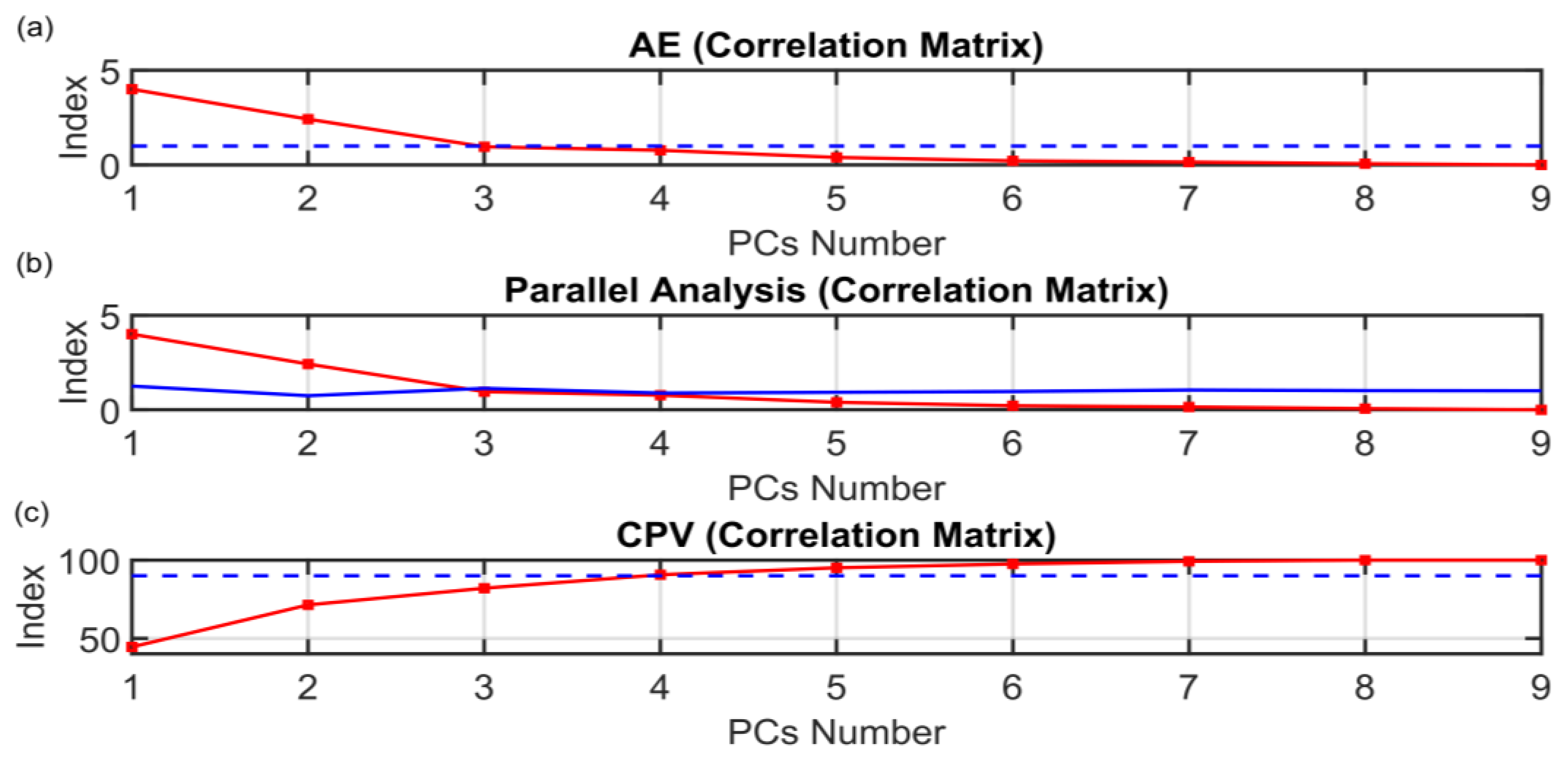
2.3. PCs Selection
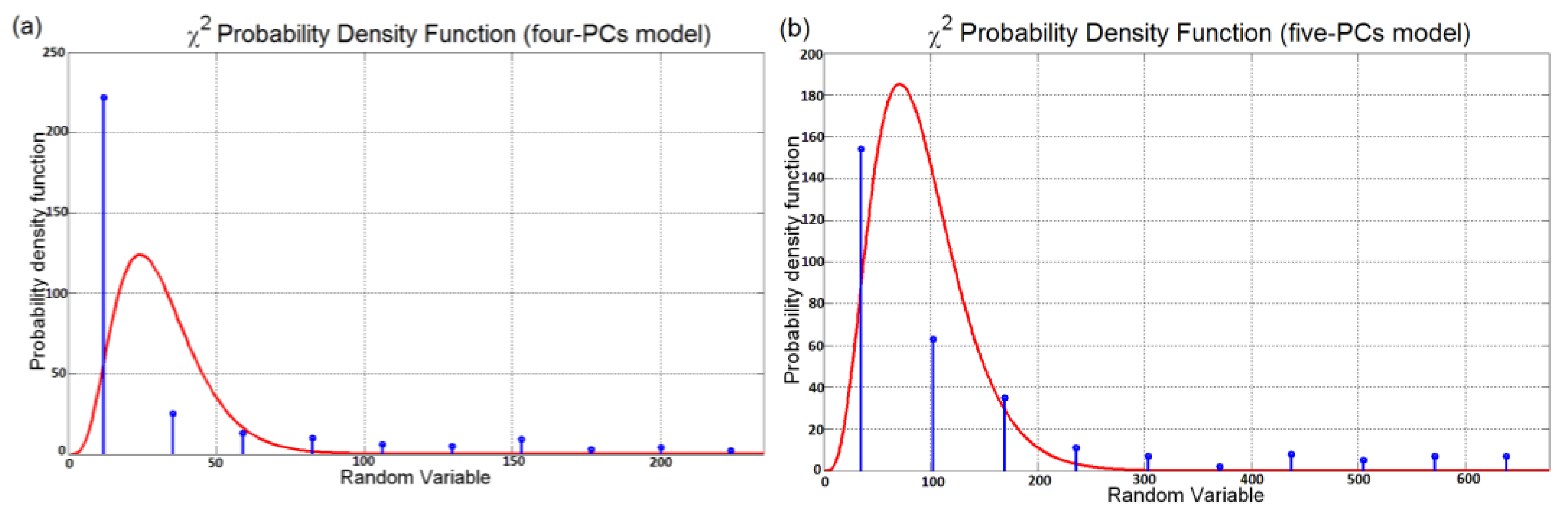
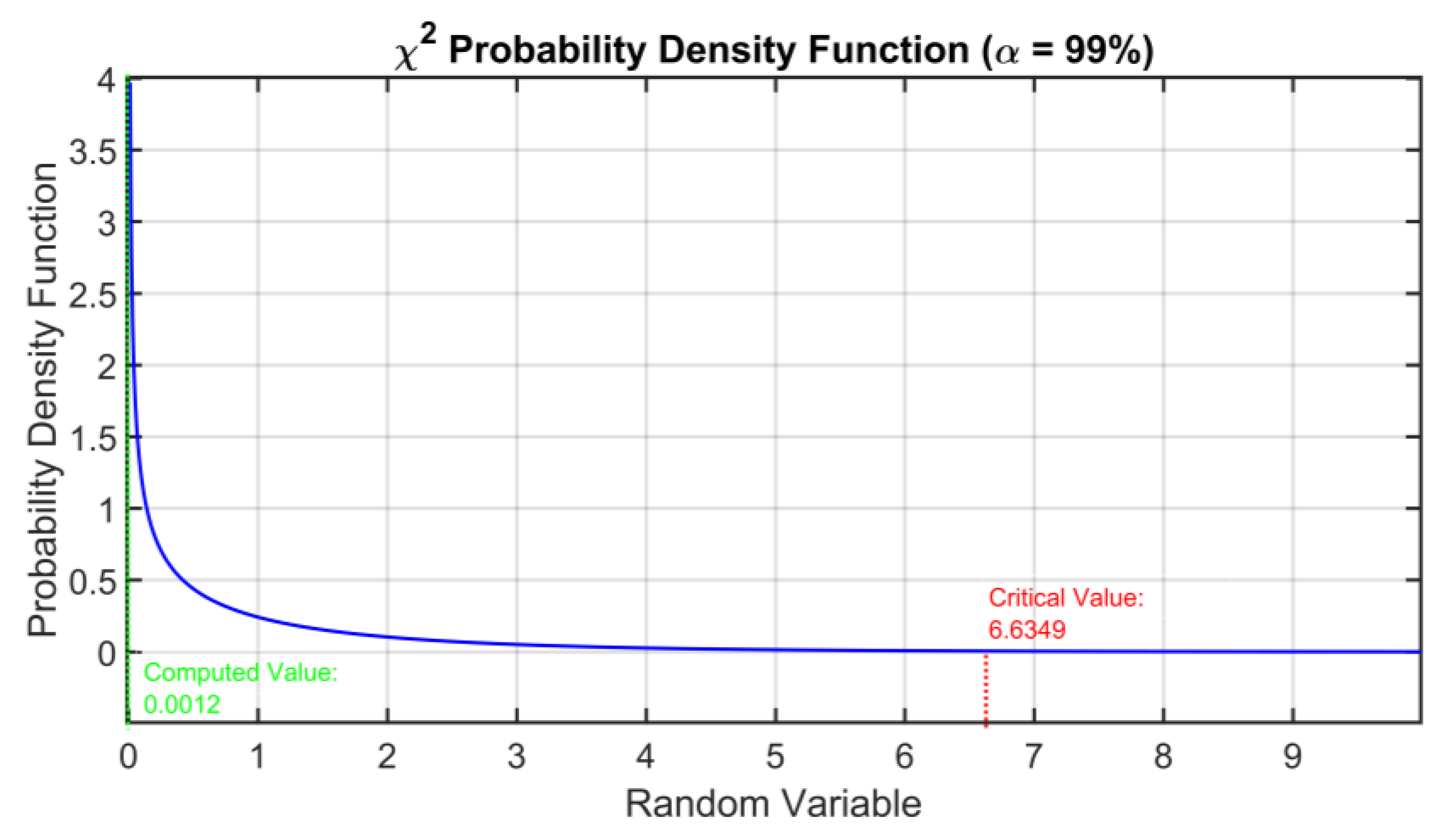
- A normal distribution characterized by a zero mean and variance σ2 must represent the reconstruction errors; if this assumption is satisfied, the denominator and the numerator of the statistical index F can be represented through a χ2 distribution as defined by Fisher’s test [70].
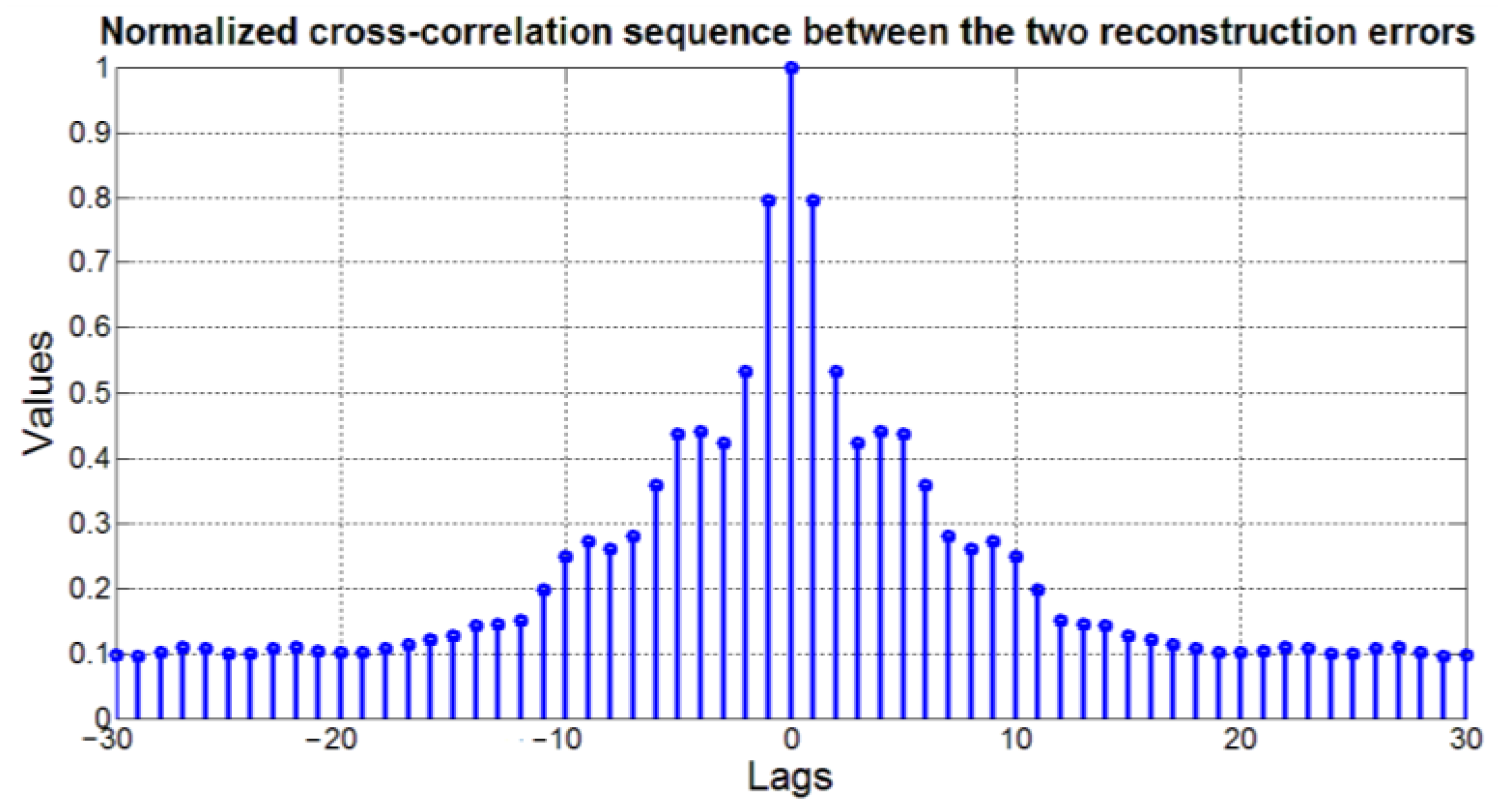
- The reconstruction errors must be independent.
- The variance of the reconstruction errors should be the same (homoscedasticity property).
2.3.1. Index of Reconstruction Error
- If errors associated to variables must be represented by a Gaussian distribution with a zero mean and variance σ2, the sum of the squared errors must follow a χ2 distribution with n degrees of freedom (where n is the number of the error vectors composing the sum).
- If errors associated to each model are characterized by the same variance, the sum of the squared errors exhibit the same variance.
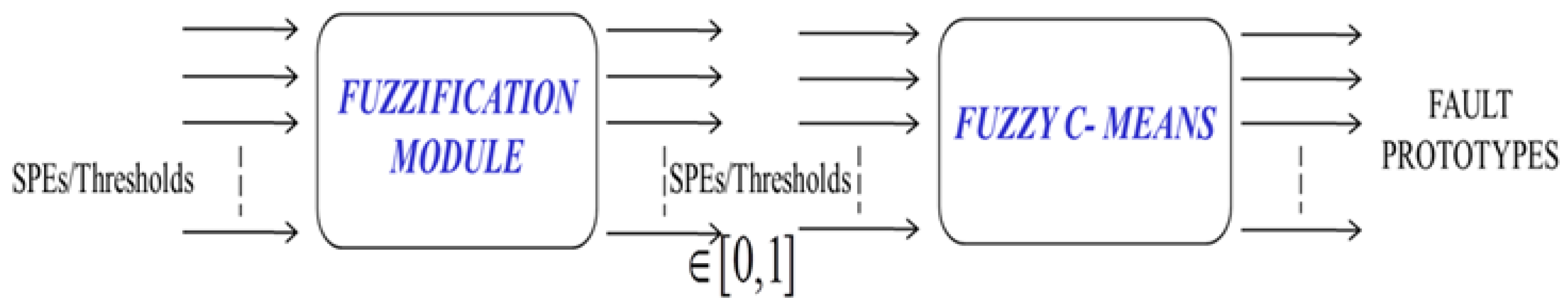
2.4. Fuzzy Faults Classifier (FFC)
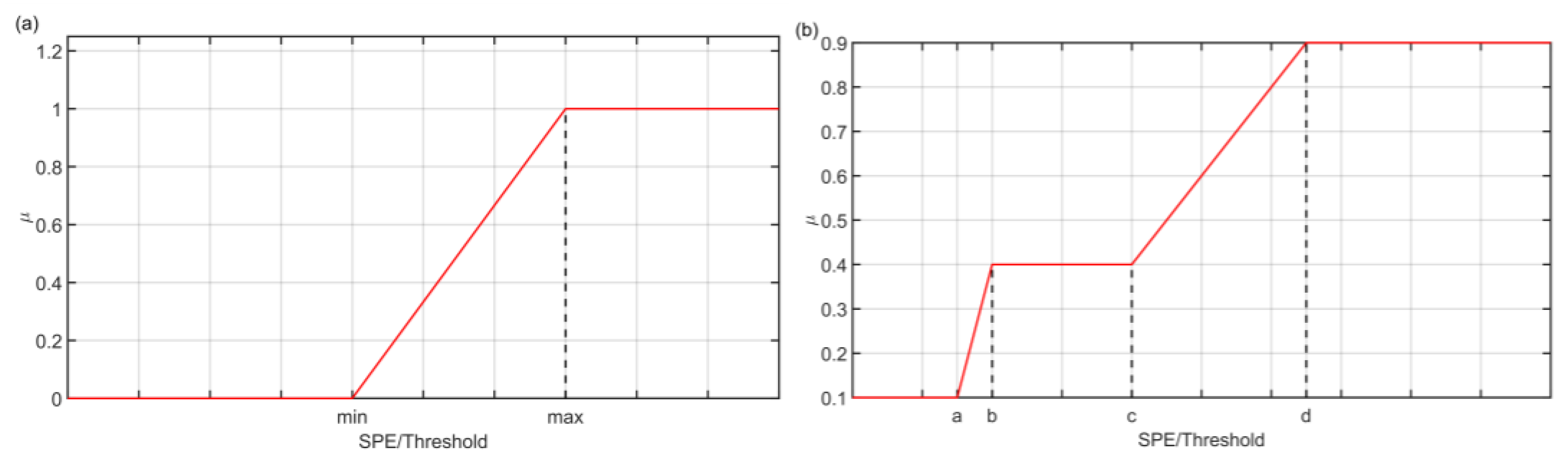
2.4.1. Fuzzification
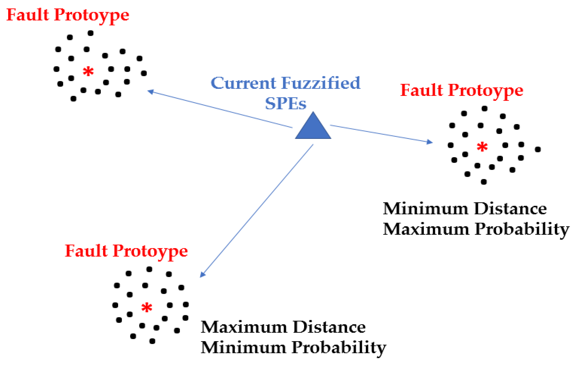
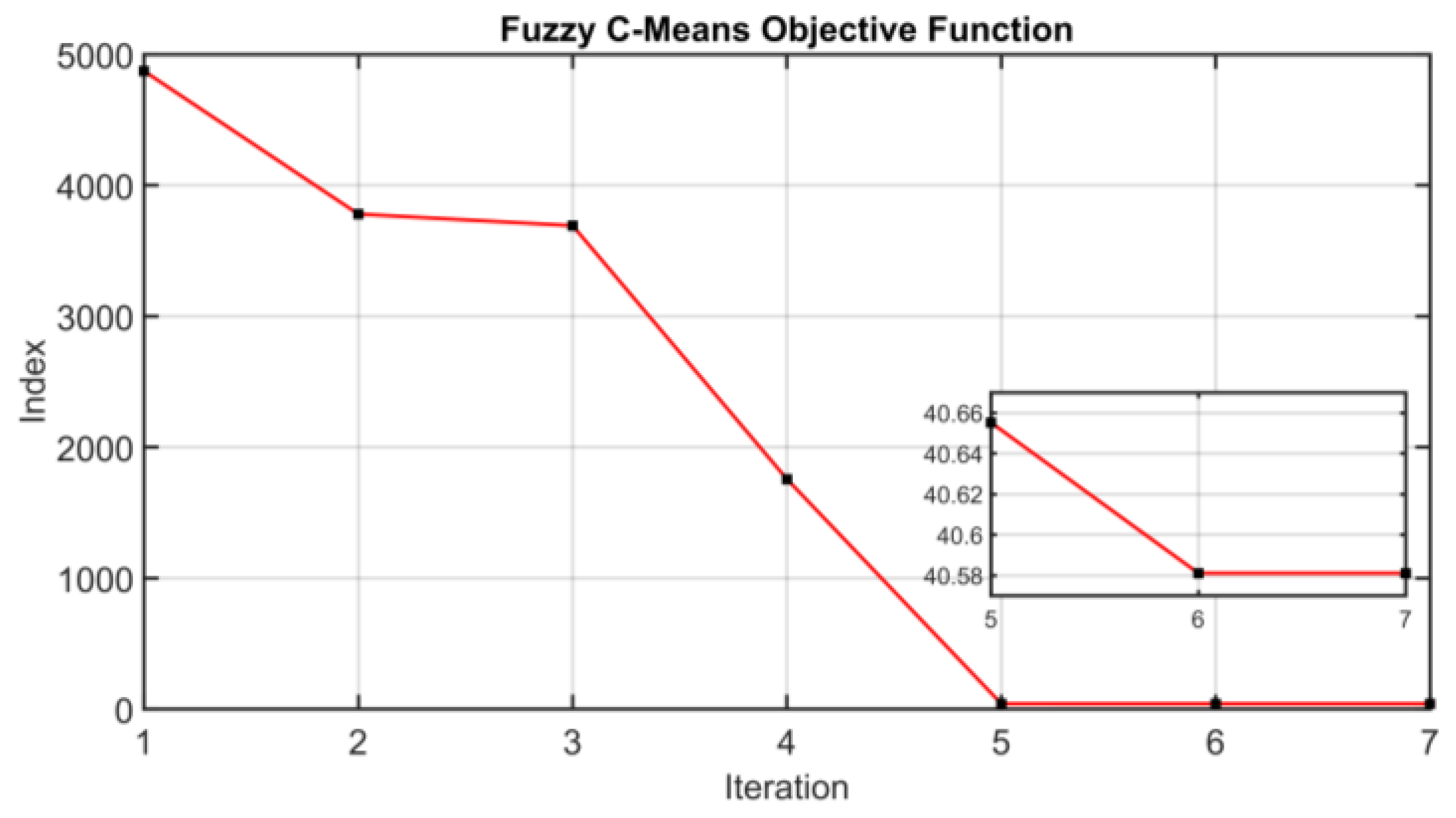
2.4.2. Cluster Analysis Procedure
2.4.3. False Alarms and Chattering Avoidance
2.5. FDI Framework Computational Architecture
2.6. Comparison between the Proposed FDI Framework and Other Procedures
3. Results and Discussion
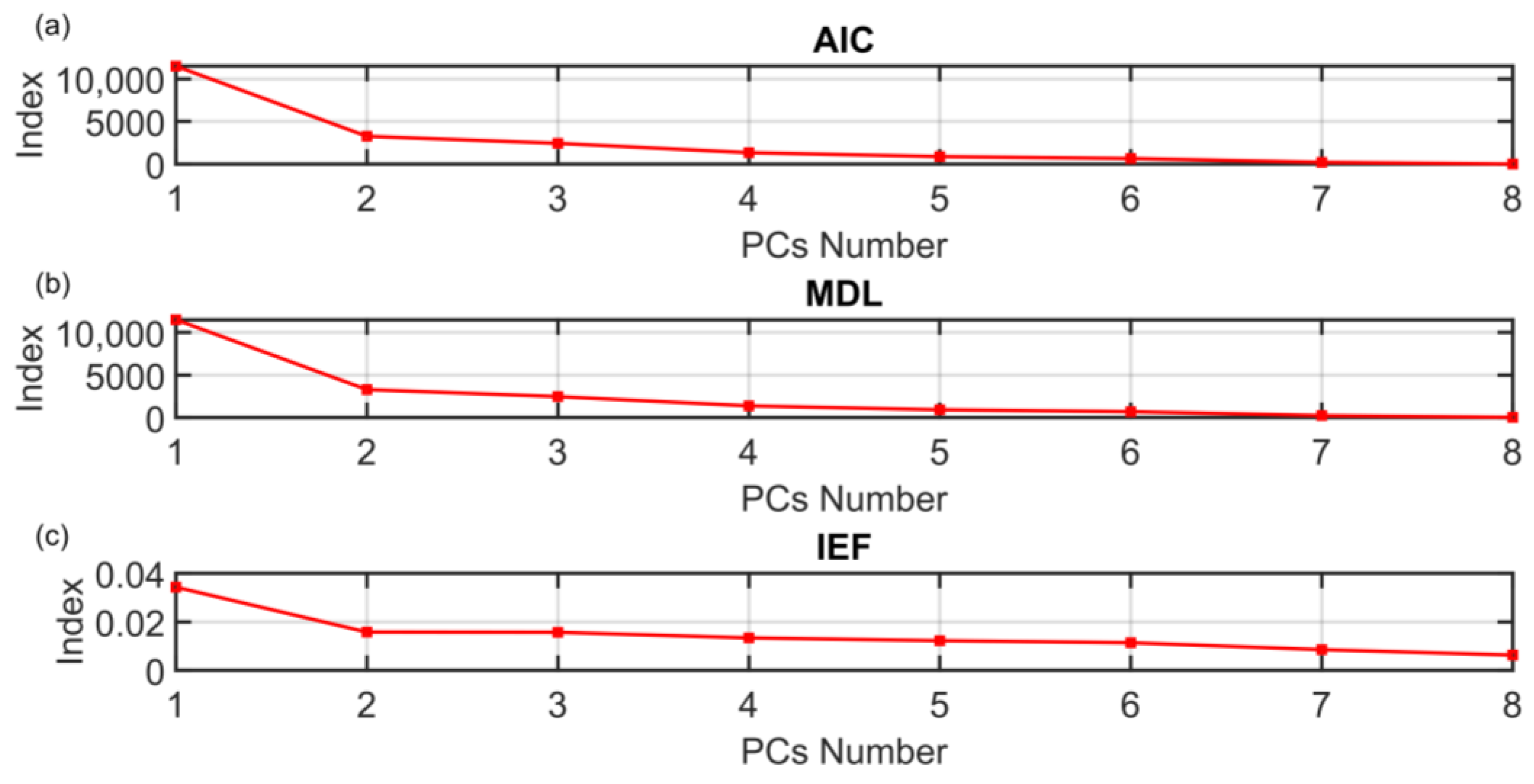
3.1. ANOVA Test PCs Selection Results
3.2. Comparison between the ANOVA Test PCs Selection Method and Other Methods
3.3. Results on Fuzzification and Cluster Analysis
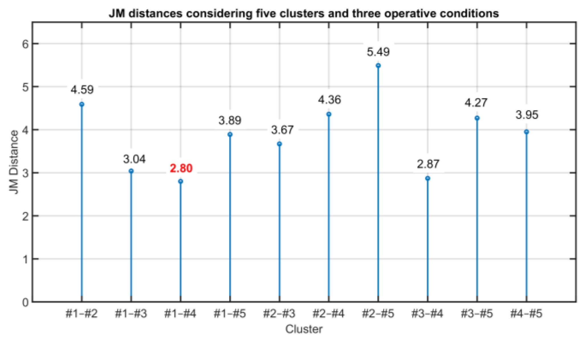
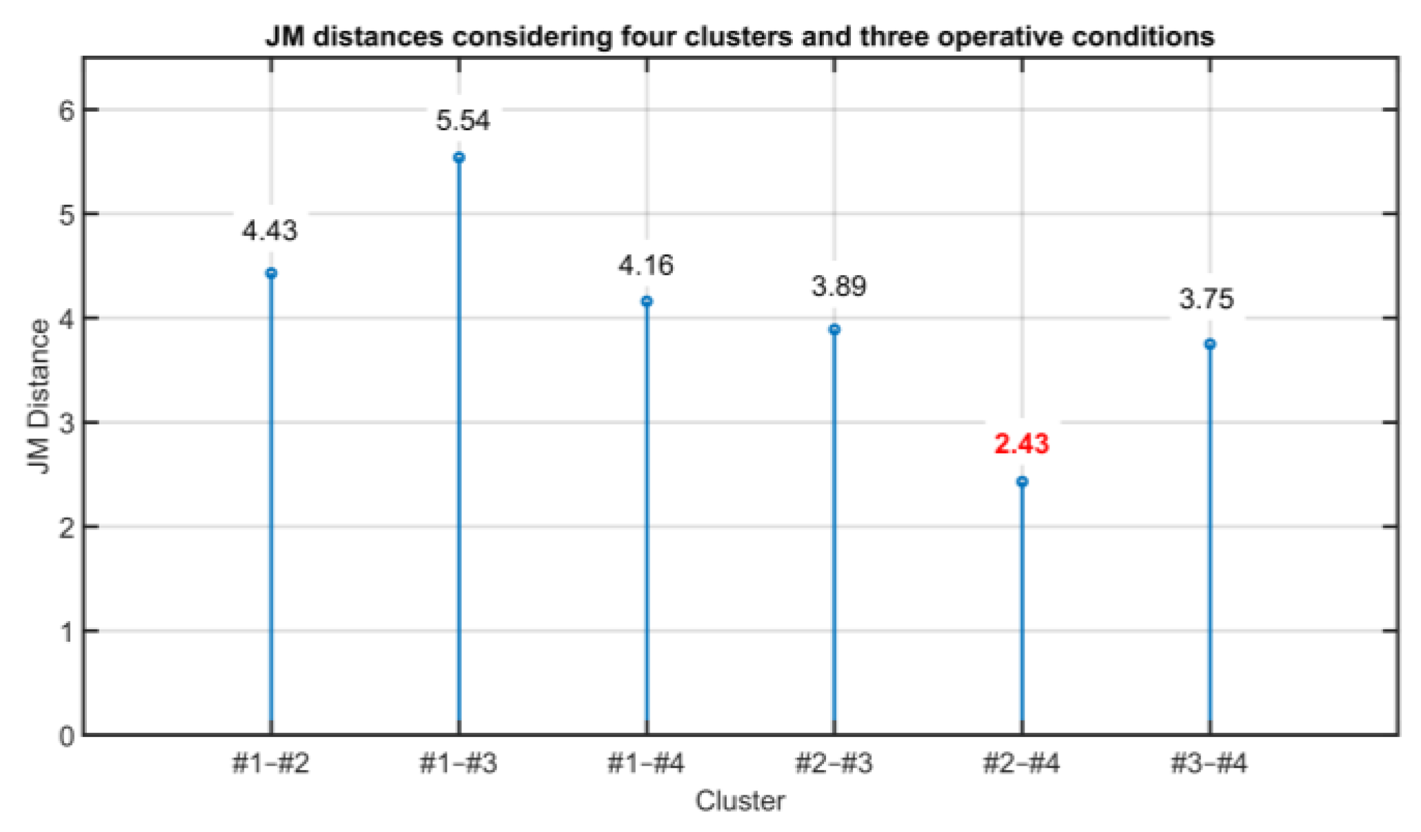
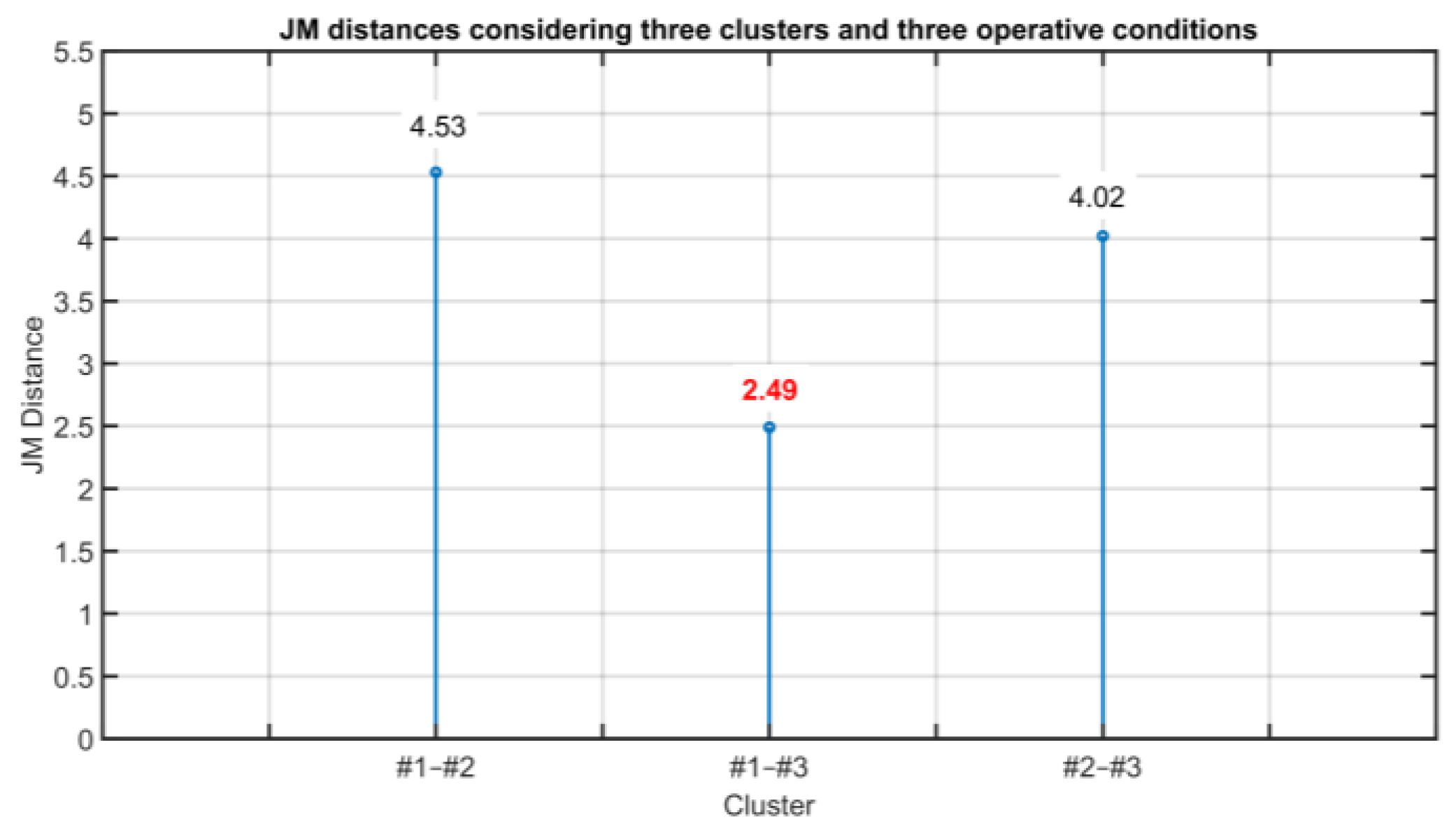
3.4. Results on the Validation of the Clustering Consistency
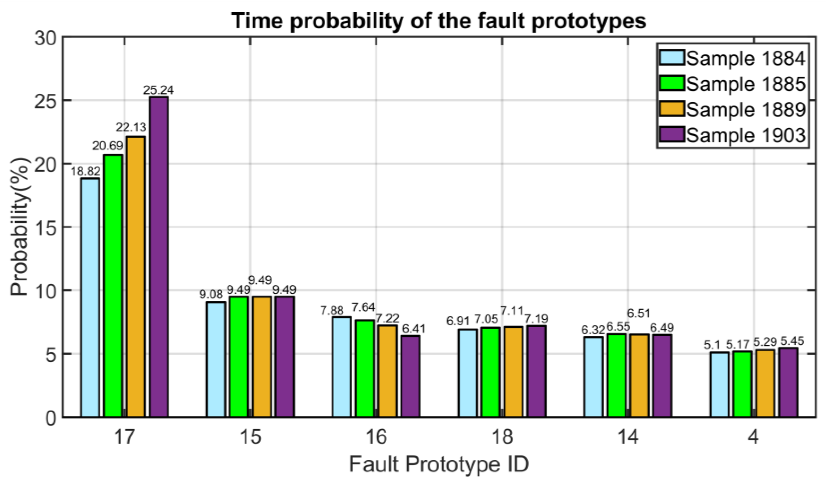
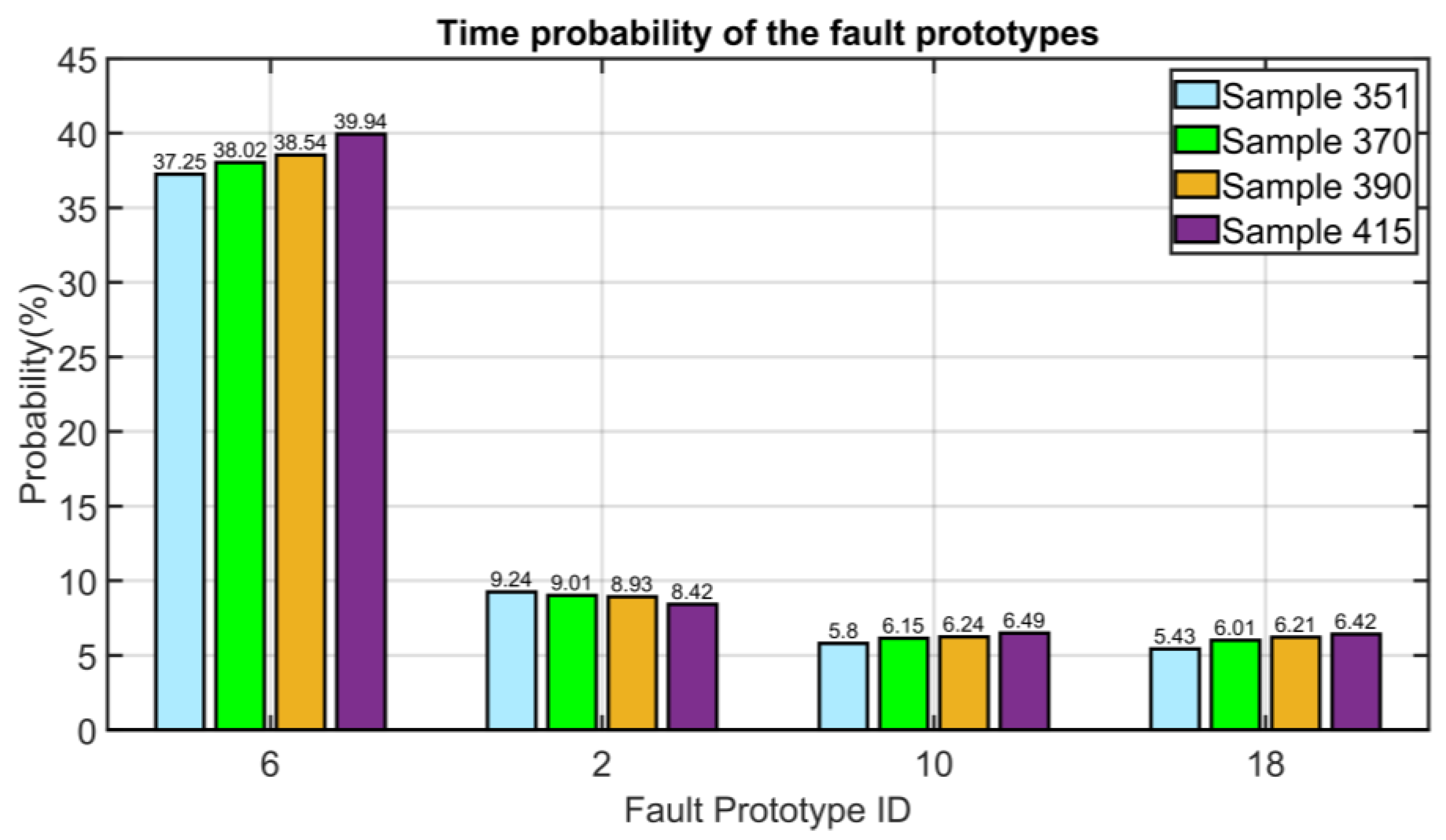
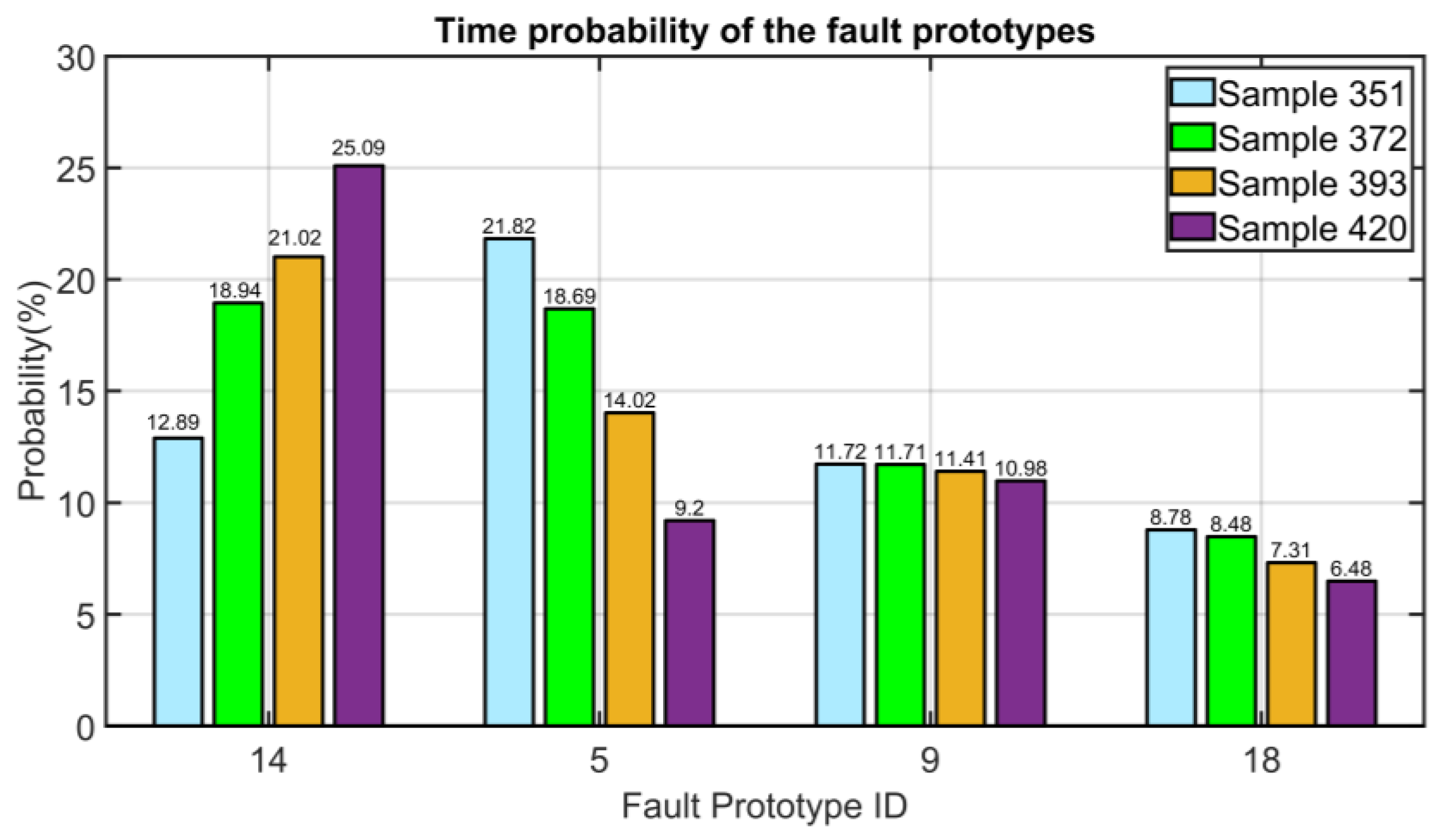
3.5. Results on NMSC FDI
3.5.1. Process Fault: Fouling of the Compressor Stage
3.5.2. Instrument Single Fault: Error on Thermocouple Relative to the First Stage Bearing (PV13)
3.5.3. Instrument Multiple Faults: Simultaneous Error on the Vibration’s Measurements (PV14 and PV15)
4. Conclusions
Author Contributions
Funding
Institutional Review Board Statement
Informed Consent Statement
Data Availability Statement
Conflicts of Interest
References
- Zanoli, S.M.; Pepe, C.; Barboni, L. Application of Advanced Process Control techniques to a pusher type reheating furnace. J. Phys. Conf. Ser. 2015, 659, 012014. [Google Scholar] [CrossRef]
- Zanoli, S.M.; Astolfi, G.; Orlietti, L.; Frisinghelli, M.; Pepe, C. Water Distribution Networks Optimization: A real case study. IFAC-PapersOnLine 2020, 53, 16644–16650. [Google Scholar] [CrossRef]
- Zanoli, S.M.; Pepe, C.; Astolfi, G. Advanced Process Control of a cement plant grate cooler. In Proceedings of the 2022 26th International Conference on System Theory, Control and Computing (ICSTCC), Sinaia, Romania, 19–21 October 2022. [Google Scholar] [CrossRef]
- Zanoli, S.M.; Cocchioni, F.; Pepe, C. Model Predictive Control with horizons online adaptation: A steel industry case study. In Proceedings of the 2018 European Control Conference (ECC), Limassol, Cyprus, 12–15 June 2018. [Google Scholar] [CrossRef]
- Bundesministerium für Wirtschaft und Klimaschutz. Available online: https://www.plattform-i40.de/ (accessed on 30 November 2022).
- Vaidya, S.; Ambad, P.; Bhosle, S. Industry 4.0—A Glimpse. Procedia Manuf. 2018, 20, 233–238. [Google Scholar] [CrossRef]
- Pereira, A.C.; Romero, F. A review of the meanings and the implications of the Industry 4.0 concept. Procedia Manuf. 2017, 13, 1206–1214. [Google Scholar] [CrossRef]
- Jasiulewicz-Kaczmarek, M.; Gola, A. Maintenance 4.0 Technologies for Sustainable Manufacturing—An Overview. IFAC-PapersOnLine 2019, 52, 91–96. [Google Scholar] [CrossRef]
- Silvestri, L.; Forcina, A.; Introna, V.; Santolamazza, A.; Cesarotti, V. Maintenance transformation through Industry 4.0 technologies: A systematic literature review. Comput. Ind. 2020, 123, 103335. [Google Scholar] [CrossRef]
- Zanoli, S.M.; Pepe, C.; Moscoloni, E.; Astolfi, G. Data Analysis and Modelling of Billets Features in Steel Industry. Sensors 2022, 22, 7333. [Google Scholar] [CrossRef]
- Sabbatini, L.; Belli, A.; Palma, L.; Pierleoni, P. One datum and many values for sustainable Industry 4.0: A prognostic and health management use case. Int. J. Electr. Comput. Eng. 2023, 13, 658–668. [Google Scholar] [CrossRef]
- Zanoli, S.M.; Barboni, L.; Cocchioni, F.; Pepe, C. Advanced process control aimed at energy efficiency improvement in process industries. In Proceedings of the 2018 IEEE International Conference on Industrial Technology (ICIT), Lyon, France, 20–22 February 2018. [Google Scholar] [CrossRef]
- Zanoli, S.M.; Cocchioni, F.; Pepe, C. MPC-based energy efficiency improvement in a pusher type billets reheating furnace. Adv. Sci. Technol. Eng. Syst. J. 2018, 3, 74–84. [Google Scholar] [CrossRef] [Green Version]
- Zanoli, S.M.; Pepe, C.; Rocchi, M.; Astolfi, G. Application of Advanced Process Control techniques for a cement rotary kiln. In Proceedings of the 2015 19th International Conference on System Theory, Control and Computing (ICSTCC), Cheile Gradistei, Romania, 14–16 October 2015. [Google Scholar] [CrossRef]
- Zanoli, S.M.; Pepe, C.; Orlietti, L.; Barchiesi, D. A Model Predictive Control strategy for energy saving and user comfort features in building automation. In Proceedings of the 2015 19th International Conference on System Theory, Control and Computing (ICSTCC), Cheile Gradistei, Romania, 14–16 October 2015. [Google Scholar] [CrossRef]
- Zanoli, S.M.; Pepe, C. A constraints softening decoupling strategy oriented to time delays handling with Model Predictive Control. In Proceedings of the 2016 American Control Conference (ACC), Boston, MA, USA, 6–8 July 2016. [Google Scholar] [CrossRef]
- Patton, R.J.; Frank, P.M.; Clarke, R.N. Fault Diagnosis in Dynamic Systems: Theory and Application; Prentice-Hall: Upper Saddle River, NJ, USA, 1989. [Google Scholar]
- Isermann, R. Fault-Diagnosis Systems—An Introduction from Fault Detection to Fault Tolerance; Springer: Berlin/Heidelberg, Germany, 2006. [Google Scholar] [CrossRef]
- Isermann, R. Fault-Diagnosis Applications—Model-Based Condition Monitoring: Actuators, Drives, Machinery, Plants, Sensors, and Fault-Tolerant Systems; Springer: Berlin/Heidelberg, Germany, 2011. [Google Scholar] [CrossRef]
- Zanoli, S.M.; Astolfi, G. Application of a Fault Detection and Isolation System on a Rotary Machine. Int. J. Rotating Mach. 2013, 2013, 189359. [Google Scholar] [CrossRef] [Green Version]
- Tharrault, Y.; Mourot, G.; Ragot, J. Fault detection and isolation with robust principal component analysis. In Proceedings of the 2008 16th Mediterranean Conference on Control and Automation, Ajaccio, France, 25–27 June 2008. [Google Scholar] [CrossRef] [Green Version]
- Talebi, H.A.; Khorasani, K.; Tafazoli, S. A Recurrent Neural-Network-Based Sensor and Actuator Fault Detection and Isolation for Nonlinear Systems with Application to the Satellite’s Attitude Control Subsystem. IEEE Trans. Neural Netw. 2009, 20, 45–60. [Google Scholar] [CrossRef] [PubMed]
- Talebi, H.A.; Khorasani, K. A Neural Network-Based Multiplicative Actuator Fault Detection and Isolation of Nonlinear Systems. IEEE Trans. Control. Syst. Technol. 2013, 21, 842–851. [Google Scholar] [CrossRef]
- Adouni, A.; Ben Hamed, M.; Flah, A.; Sbita, L. Sensor and actuator fault detection and isolation based on artificial neural networks and fuzzy logic applicated on induction motor. In Proceedings of the 2013 International Conference on Control, Decision and Information Technologies, Hammamet, Tunisia, 6–8 May 2013. [Google Scholar] [CrossRef]
- Wang, H.; Song, Z.; Li, P. Fault Detection Behavior and Performance Analysis of Principal Component Analysis Based Process Monitoring Methods. Ind. Eng. Chem. Res. 2002, 41, 2455–2464. [Google Scholar] [CrossRef]
- Shin, B.S.; Lee, C.J.; Lee, G.; Yoon, E.S. Application of fault diagnosis based on signed digraphs and PCA with linear fault boundary. In Proceedings of the 2007 International Conference on Control, Automation and Systems, Seoul, Republic of Korea, 17–20 October 2007. [Google Scholar] [CrossRef]
- Cherry, G.A.; Qin, S.J. Multiblock principal component analysis based on a combined index for semiconductor fault detection and diagnosis. IEEE Trans. Semicond. Manuf. 2006, 19, 159–172. [Google Scholar] [CrossRef]
- Drif, M.; Marques Cardoso, A.J. Discriminating the Simultaneous Occurrence of Three-Phase Induction Motor Rotor Faults and Mechanical Load Oscillations by the Instantaneous Active and Reactive Power Media Signature Analyses. IEEE Trans. Ind. Electron. 2012, 59, 1630–1639. [Google Scholar] [CrossRef]
- Pierleoni, P.; Palma, L.; Belli, A.; Sabbatini, L. Using Plastic Injection Moulding Machine Process Parameters for Predictive Maintenance Purposes. In Proceedings of the 2020 International Conference on Intelligent Engineering and Management (ICIEM), London, UK, 17–19 June 2020. [Google Scholar] [CrossRef]
- Ghate, V.N.; Dudul, S.V. Cascade Neural-Network-Based Fault Classifier for Three-Phase Induction Motor. IEEE Trans. Ind. Electron. 2011, 58, 1555–1563. [Google Scholar] [CrossRef]
- Frosini, L.; Bassi, E. Stator Current and Motor Efficiency as Indicators for Different Types of Bearing Faults in Induction Motors. IEEE Trans. Ind. Electron. 2009, 57, 244–251. [Google Scholar] [CrossRef]
- Choqueuse, V.; Benbouzid, M.E.H.; Amirat, Y.; Turri, S. Diagnosis of Three-Phase Electrical Machines Using Multidimensional Demodulation Techniques. IEEE Trans. Ind. Electron. 2012, 59, 2014–2023. [Google Scholar] [CrossRef] [Green Version]
- Martins, J.F.; Ferno Pires, V.; Pires, A.J. Unsupervised Neural-Network-Based Algorithm for an On-Line Diagnosis of Three-Phase Induction Motor Stator Fault. IEEE Trans. Ind. Electron. 2007, 54, 259–264. [Google Scholar] [CrossRef]
- Fernão Pires, V.; Martins, J.F.; Pires, A.J. Eigenvector/eigenvalue analysis of a 3D current referential fault detection and diagnosis of an induction motor. Energy Convers. Manag. 2010, 51, 901–907. [Google Scholar] [CrossRef]
- Kim, M.-C.; Lee, J.-H.; Wang, D.-H.; Lee, I.-S. Induction Motor Fault Diagnosis Using Support Vector Machine, Neural Networks, and Boosting Methods. Sensors 2023, 23, 2585. [Google Scholar] [CrossRef]
- Yang, Y.; Haque, M.M.M.; Bai, D.; Tang, W. Fault Diagnosis of Electric Motors Using Deep Learning Algorithms and Its Application: A Review. Energies 2021, 14, 7017. [Google Scholar] [CrossRef]
- Joung, B.G.; Lee, W.J.; Huang, A.; Sutherland, J.W. Development and Application of a Method for Real Time Motor Fault Detection. Procedia Manuf. 2020, 49, 94–98. [Google Scholar] [CrossRef]
- Ince, T.; Kiranyaz, S.; Eren, L.; Askar, M.; Gabbouj, M. Real-Time Motor Fault Detection by 1-D Convolutional Neural Networks. IEEE Trans. Ind. Electron. 2016, 63, 7067–7075. [Google Scholar] [CrossRef]
- Ágoston, K. Fault Detection of the Electrical Motors Based on Vibration Analysis. Procedia Technol. 2015, 19, 547–553. [Google Scholar] [CrossRef] [Green Version]
- Isermann, R.; Nold, S. Model Based Fault Detection for Centrifugal Pumps and AC Drives. In Proceedings of the 11th IMEKO World Congress, Houston, TX, USA, 16–21 October 1988. [Google Scholar]
- Higham, E.H.; Perovic, S. Predictive maintenance of pumps based on signal analysis of pressure and differential pressure (flow) measurements. Trans. Inst. Meas. Control. 2001, 23, 226–248. [Google Scholar] [CrossRef]
- Dalton, T.; Patton, R. Model-based fault diagnosis of a two-pump system. Trans. Inst. Meas. Control. 1998, 20, 115–124. [Google Scholar] [CrossRef]
- Ahmad, S.; Ahmad, Z.; Kim, J.-M. A Centrifugal Pump Fault Diagnosis Framework Based on Supervised Contrastive Learning. Sensors 2022, 22, 6448. [Google Scholar] [CrossRef] [PubMed]
- Ahmad, Z.; Nguyen, T.-K.; Ahmad, S.; Nguyen, C.D.; Kim, J.-M. Multistage Centrifugal Pump Fault Diagnosis Using Informative Ratio Principal Component Analysis. Sensors 2022, 22, 179. [Google Scholar] [CrossRef]
- Prosvirin, A.E.; Ahmad, Z.; Kim, J.-M. Global and Local Feature Extraction Using a Convolutional Autoencoder and Neural Networks for Diagnosing Centrifugal Pump Mechanical Faults. IEEE Access 2021, 9, 65838–65854. [Google Scholar] [CrossRef]
- Ahmad, Z.; Rai, A.; Hasan, M.J.; Kim, C.H.; Kim, J.-M. A Novel Framework for Centrifugal Pump Fault Diagnosis by Selecting Fault Characteristic Coefficients of Walsh Transform and Cosine Linear Discriminant Analysis. IEEE Access 2021, 9, 150128–150141. [Google Scholar] [CrossRef]
- Hasan, M.J.; Rai, A.; Ahmad, Z.; Kim, J.-M. A Fault Diagnosis Framework for Centrifugal Pumps by Scalogram-Based Imaging and Deep Learning. IEEE Access 2021, 9, 58052–58066. [Google Scholar] [CrossRef]
- Bahadori, A. Natural Gas Processing—Technology and Engineering Design; Elsevier: Amsterdam, The Netherlands, 2014. [Google Scholar] [CrossRef]
- Ferguson, T.B. The Centrifugal Compressor Stage; Butterworths: London, UK, 1963. [Google Scholar]
- Wood, B.M.; Olsen, C.L.; Hartzo, G.D.; Rama, J.C.; Szenasi, F.R. Development of an 11,000-r/min 3500-HP induction motor and adjustable-speed drive for refinery service. IEEE Trans. Ind. Appl. 1997, 33, 815–825. [Google Scholar] [CrossRef]
- Liaw, D.C.; Song, C.C.; Huang, J.T. Robust Stabilization of a Centrifugal Compressor with Spool Dynamics. IEEE Trans. Control. Syst. Technol. 2004, 12, 966–972. [Google Scholar] [CrossRef]
- de Jager, B. Rotating stall and surge control: A survey. In Proceedings of the 1995 34th IEEE Conference on Decision and Control, New Orleans, LA, USA, 13–15 December 1995. [Google Scholar] [CrossRef] [Green Version]
- Gravdahl, J.T.; Egeland, O. Centrifugal compressor surge and speed control. IEEE Trans. Control. Syst. Technol. 1999, 7, 567–579. [Google Scholar] [CrossRef]
- Gravdahl, J.T.; Egeland, O. Speed and surge control for a low order centrifugal compressor model. In Proceedings of the 1997 IEEE International Conference on Control Applications, Hartford, CT, USA, 5–7 October 1997. [Google Scholar] [CrossRef] [Green Version]
- Wang, C.; Shao, C.; Han, Y. Centrifugal compressor surge control using nonlinear model predictive control based on LS-SVM. In Proceedings of the 2010 3rd International Symposium on Systems and Control in Aeronautics and Astronautics, Harbin, China, 8–10 June 2010. [Google Scholar] [CrossRef]
- Gravdahl, J.T.; Egeland, O. Compressor Surge and Rotating Stall—Modeling and Control; Springer: London, UK, 1999. [Google Scholar]
- Liao, H.-J.; Huang, S.-Z. The fault diagnosis for centrifugal compressor based on time series analysis with neural network. In Proceedings of the 2010 3rd International Conference on Advanced Computer Theory and Engineering (ICACTE), Chengdu, China, 20–22 August 2010. [Google Scholar] [CrossRef]
- Me, Z.; Guo, H.; Duan, L. New Method to Establish Fault Diagnostic Standard of Centrifugal Compressor. Oil Field Equipment 2010, 8, 65–68. [Google Scholar]
- Yu, X.H.; Zhang, L.B.; Wang, Z. Fault Diagnosis of Refrigerator Compressor on the Vibrating Spectral Analysis. Oil Field Equipment 2005, 34, 19–23. [Google Scholar]
- Mugnaini, M.; Quercioli, V.; Catelani, M.; Singuaroli, R.; Fort, A. Characterization of centrifugal compressors’ thermo-elements used in journal and thrust bearing temperature monitoring. In Proceedings of the 19th IEEE Instrumentation and Measurement Technology Conference (IEEE Cat. No.00CH37276), Anchorage, AK, USA, 21–23 May 2002. [Google Scholar] [CrossRef]
- Nordal, H.; El-Thalji, I. Assessing the Technical Specifications of Predictive Maintenance: A Case Study of Centrifugal Compressor. Appl. Sci. 2021, 11, 1527. [Google Scholar] [CrossRef]
- Sonthipo, T.; Ardsomang, T.; Chancharoen, R. Fault detection and identification for centrifugal compressor by ensemble model. In Proceedings of the 2022 37th International Technical Conference on Circuits/Systems, Computers and Communications (ITC-CSCC), Phuket, Thailand, 5–8 July 2022. [Google Scholar] [CrossRef]
- Lu, Y.; Wang, F.; Jia, M.; Qi, Y. Centrifugal compressor fault diagnosis based on qualitative simulation and thermal parameters. Mech. Syst. Signal Process. 2016, 81, 259–273. [Google Scholar] [CrossRef]
- Li, X.; Duan, F.; Loukopoulos, P.; Bennett, I.; Mba, D. Canonical variable analysis and long short-term memory for fault diagnosis and performance estimation of a centrifugal compressor. Control. Eng. Pract. 2018, 72, 177–191. [Google Scholar] [CrossRef]
- Libeyre, F.; Bainier, F.; Alas, P. A Comprehensive Modeling of Centrifugal Compressor Vibrations for Early Fault Detection. In Proceedings of the ASME Turbo Expo 2020: Turbomachinery Technical Conference and Exposition. Volume 5: Controls, Diagnostics, and Instrumentation; Cycle Innovations; Cycle Innovations: Energy Storage, Virtual, 21–25 September 2020. [Google Scholar] [CrossRef]
- Nail, B.; Hadroug, N.; Hafaifa, A.; Kouzou, A. Fault Detection and Localization of Centrifugal Gas Compressor System Using Fuzzy Logic and Hybrid Kernel-SVM Methods. In Diagnosis, Fault Detection & Tolerant Control. Studies in Systems, Decision and Control; Derbel, N., Ghommam, J., Zhu, Q., Eds.; Springer: Singapore, 2020; Volume 269. [Google Scholar] [CrossRef]
- Jackson, J.E. A User’s Guide to Principal Components; John Wiley & Sons: Hoboken, NJ, USA, 1991. [Google Scholar]
- Dunia, R.; Qin, S.J. Subspace approach to multidimensional fault identification and reconstruction. AIChE J. 1998, 44, 1813–1831. [Google Scholar] [CrossRef]
- Berjaga, X.; Meléndez, J.; Barta, C. Statistical fault detection and reconstruction of sensors of the Ariane engine. In Proceedings of the 18th Mediterranean Conference on Control and Automation, Marrakech, Morocco, 23–25 June 2010. [Google Scholar] [CrossRef]
- Miller, R.G. Beyond ANOVA—Basics of Applied Statistics; Chapman & Hall/CRC: Boca Raton, FL, USA, 1997. [Google Scholar]
- Malinowski, E.R. Factor Analysis in Chemistry; Wiley: New York, NY, USA, 1991. [Google Scholar]
- Kaiser, H.F. The Application of Electronic Computers to Factor Analysis. Educ. Psychol. Meas. 1960, 20, 141–151. [Google Scholar] [CrossRef]
- Horn, J.L. A rationale and test for the number of factors in factor analysis. Psychometrika 1965, 30, 179–185. [Google Scholar] [CrossRef] [PubMed]
- Cattell, R.B. The Scree Test for The Number Of Factors. Multivar. Behav. Res. 1966, 1, 245–276. [Google Scholar] [CrossRef]
- Shrager, R.I.; Hendler, R.W. Titration of individual components in a mixture with resolution of difference spectra, pKs, and redox transitions. Anal. Chem. 1982, 54, 1147–1152. [Google Scholar] [CrossRef]
- Akaike, H. Information Theory and an Extension of the Maximum Likelihood Principle. In Selected Papers of Hirotugu Akaike; Parzen, E., Tanabe, K., Kitagawa, G., Eds.; Springer: New York, NY, USA, 1998. [Google Scholar] [CrossRef]
- Rissanen, J. Modeling by shortest data description. Automatica 1978, 14, 465–471. [Google Scholar] [CrossRef]
- Malinowski, E.R. Determination of the number of factors and the experimental error in a data matrix. Anal. Chem. 1977, 49, 612–617. [Google Scholar] [CrossRef]
- Qin, S.J.; Dunia, R. Determining the number of principal components for best reconstruction. J. Process Control. 2000, 10, 245–250. [Google Scholar] [CrossRef]
- Wold, S. Cross-Validatory Estimation of the Number of Components in Factor and Principal Components Models. Technometrics 1978, 20, 397–405. [Google Scholar] [CrossRef]
- Jazwinski, A.H. Stochastic Processes and Filtering Theory; Dover Publications: Mineola, NY, USA, 1970. [Google Scholar]
- Höppner, F.; Klawonn, F.; Kruse, R.; Runkler, T. Fuzzy Cluster Analysis: Methods for Classification, Data Analysis and Image Recognition; Wiley: Hoboken, NJ, USA, 1999. [Google Scholar]
- Zimmermann, H.-J. Fuzzy Sets, Decision Making, and Expert Systems; Springer: Dordrecht, The Netherlands, 1987. [Google Scholar] [CrossRef]
- Lee, C.C. Fuzzy logic in control systems: Fuzzy logic controller. I. IEEE Trans. Syst. Man Cybern. 1990, 20, 404–418. [Google Scholar] [CrossRef] [Green Version]
- Zadeh, L.A. Fuzzy sets. Inf. Control. 1965, 8, 338–353. [Google Scholar] [CrossRef] [Green Version]
- Watanabe, S. Pattern Recognition: Human and Mechanical; John Wiley & Sons: New York, NY, USA, 1985. [Google Scholar]
- Bezdek, J.C. Pattern Recognition with Fuzzy Objective Function Algorithms; Springer New York: New York, NY, USA, 1981. [Google Scholar]
- Hammah, R.E.; Curran, J.H. Optimal delineation of joint sets using a fuzzy clustering algorithm. Int. J. Rock Mech. Min. Sci. 1998, 35, 495–496. [Google Scholar] [CrossRef]
- Matusita, K. A distance and related statistics in multivariate analysis. In Multivariate Analysis; Krishnaiah, P.R., Ed.; Academic Press: New York, NY, USA, 1966; pp. 187–200. [Google Scholar]
- Xie, X.L.; Beni, G. A validity measure for fuzzy clustering. IEEE Trans. Pattern Anal. Mach. Intell. 1991, 13, 841–847. [Google Scholar] [CrossRef]
- MathWorks. Available online: https://it.mathworks.com/ (accessed on 30 November 2022).


| Fault Description | Time Dependency |
|---|---|
| Second section N2 mass flow (sensor) | incipient fault abrupt fault |
| High pressure N2 mass flow (sensor) | incipient fault abrupt fault |
| First section N2 mass flow (sensor) | incipient fault abrupt fault |
| Third stage IGV (positioner) | incipient fault intermittent fault abrupt fault |
| First stage IGV (positioner) | incipient fault intermittent fault abrupt fault |
| Fouling of the first stage of the NMSC | incipient fault |
| Breaking of the thrust bearing relative to the first stage | incipient fault |
| PV# | PV Description | Measurement Unit |
|---|---|---|
| PV1 | N2 mass flow through the first section of the NMSC | [t/h] |
| PV2 | N2 Positioner of the IGV relative to the first and second stage of NMSC | [%] |
| PV3 | Positioner Feedback of IGV position relative to the NMSC first and second stage | [%] |
| PV4 | Vent position at the entrance of first section of NMSC | [%] |
| PV5 | N2 mass flow through the second section of NMSC | [t/h] |
| PV6 | Positioner of the IGV relative to the third stage of NMSC | [%] |
| PV7 | Feedback of IGV position relative to the third stage of NMSC | [%] |
| PV8 | Throttle valve position relative to inlet high pressure nitrogen gas | [%] |
| PV9 | Compression ratio of the first stage of NMSC | [-] |
| PV10 | Polytrophic efficiency of the first stage of NMSC | [-] |
| PV11 | N2 mass flow from the head of the high-pressure column | [t/h] |
| PV12 | Power consumption by NMSC | [kW] |
| PV13 | Thrust bearing temperature of the first shaft | [°C] |
| PV14 | Horizontal vibrations of the first shaft of NMSC | [μm] |
| PV15 | Vertical vibrations of the first shaft of NMSC | [μm] |
| PV16 | Throttle valve position relative to inlet high pressure N2 gas | [%] |
| PV17 | N2 temperature at the inlet of the 5th stage of the NMSC | [°C] |
| PV18 | N2 pressure at the inlet of the 5th stage of the NMSC | [bar] |
| PV19 | N2 pressure at the exit of the heat exchanger used in the 5th stage of the NMSC | [bar] |
| PV20 | N2 temperature at the exit of the heat exchanger used in the 5th stage of the NMSC | [°C] |
| PV21 | Thrust bearing temperature of the shaft | [°C] |
| PV22 | Horizontal vibrations of the 5th shaft of NMSC | [μm] |
| PV23 | Vertical vibrations of the 5th shaft of NMSC | [μm] |
| PV24 | Thrust bearing temperature of the shaft | [°C] |
| PV25 | Thrust bearing temperature of the shaft | [°C] |
| PV26 | N2 temperature at the exit of the 5th stage of the NMSC | [°C] |
| PV27 | H2O temperature at the exit of the heat exchanger used in the 5th stage of the NMSC | [°C] |
| Fault Prototype ID | Fault Prototype Description |
|---|---|
| (1) | Absence of faults |
| (2) | Failure in the N2 mass flow sensor in the first section (PV1) |
| (3) | Error in the control of first stage IGV position (PV2) |
| (4) | Error in the horizontal vibration’s measurement (PV14) |
| (5) | Error in the vertical vibration’s measurement (PV15) |
| (6) | Fault in the thermocouple relative to the first stage bearing (PV13) |
| (7) | Simultaneous fault in the first section N2 mass flow sensor (PV1) and in the control of first stage IGV position (PV2) |
| (8) | Simultaneous fault in the first section N2 mass flow sensor (PV1) and in the horizontal vibration’s measurement (PV14) |
| (9) | Simultaneous faults in the first section N2 mass flow sensor (PV1) and in the vertical vibration’s measurement (PV15) |
| (10) | Simultaneous faults in the first section N2 mass flow sensor (PV1) and in the thermocouple relative to the first stage bearing (PV13) |
| (11) | Simultaneous faults in the control of first stage IGV position (PV2) and in the horizontal vibration’s measurement (PV14) |
| (12) | Simultaneous faults in the control of first stage IGV position (PV2) and in the vertical vibration’s measurement (PV15) |
| (13) | Simultaneous faults in the control of first stage IGV position (PV2) and in the thermocouple relative to the first stage bearing (PV13) |
| (14) | Simultaneous error in the vibration’s measurements (PV14 and PV15) |
| (15) | Simultaneous fault in the horizontal vibration’s measurement (PV14) and in the thermocouple relative to the first stage bearing (PV13) |
| (16) | Simultaneous fault in the vertical vibration’s measurement (PV15) and in the thermocouple relative to the first stage bearing (PV13) |
| (17) | Fouling of the first stage of the NMSC |
| (18) | Breaking of the thrust bearing relative to the first stage |
| Eigenvalue |
|---|
| 5687.9 |
| 4767.2 |
| 3767.0 |
| 2773.9 |
| 2036.3 |
| 1416.8 |
| 996.1 |
| 800.9 |
| 245 |
| Crucial Value | Calculated Value | Result |
|---|---|---|
| 6.6349 | 0.0012 | The assumption of equality of the variances of the reconstruction errors is fulfilled |
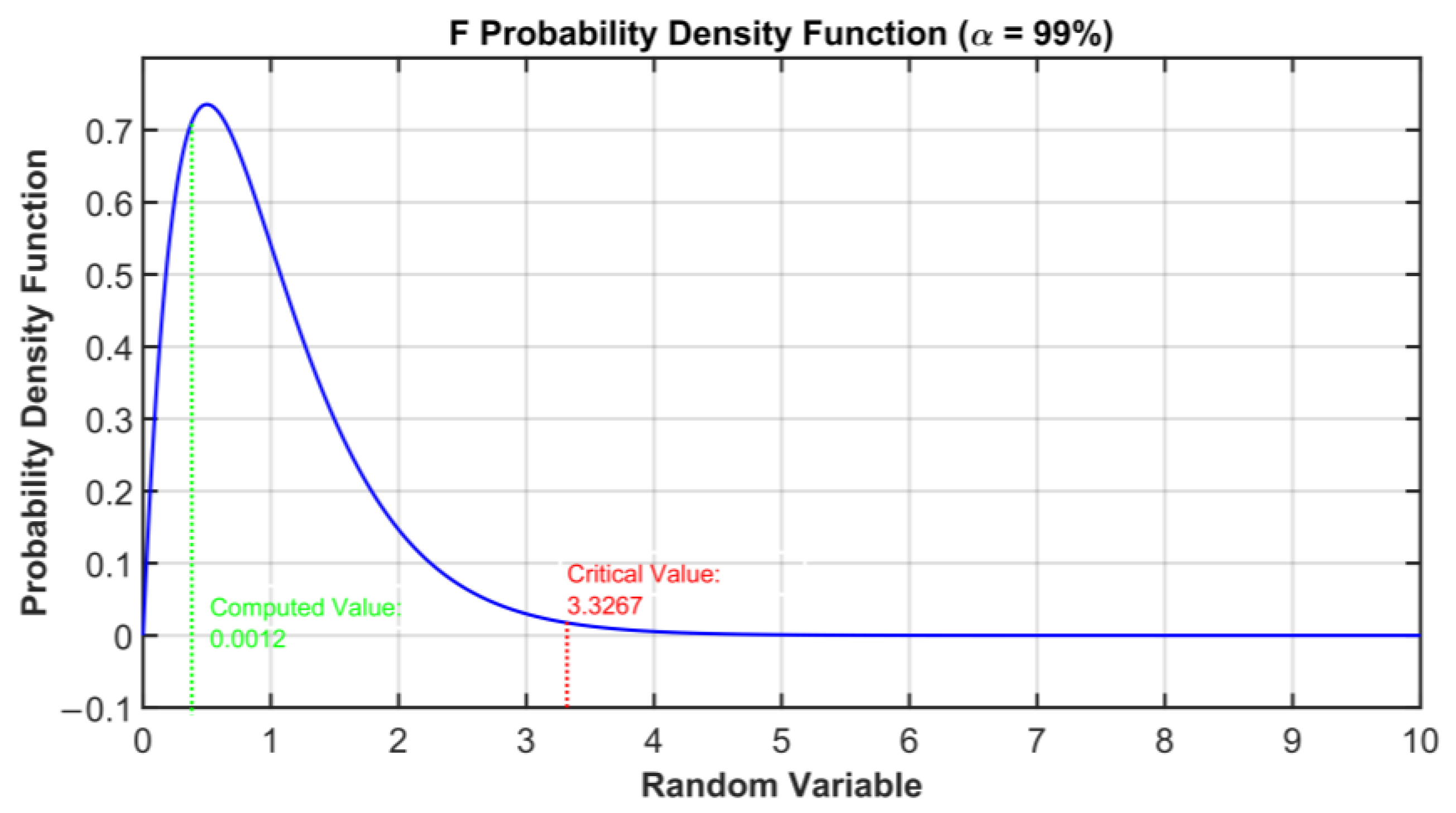
| Degree of Freedom | Sum of Squares | Mean Squares | Computed F Value | Critical F Value | Cp Mallows Index |
|---|---|---|---|---|---|
| p − 1 | 0.15 × 10⁵ | 3.67 × 10³ | 3.3267 | 0.3754 | 4.26 |
| N − p | 4.55 × 10⁵ | 1.55 × 10³ | |||
| N − 1 | 4.69 × 10⁵ | 1.57 × 10³ |
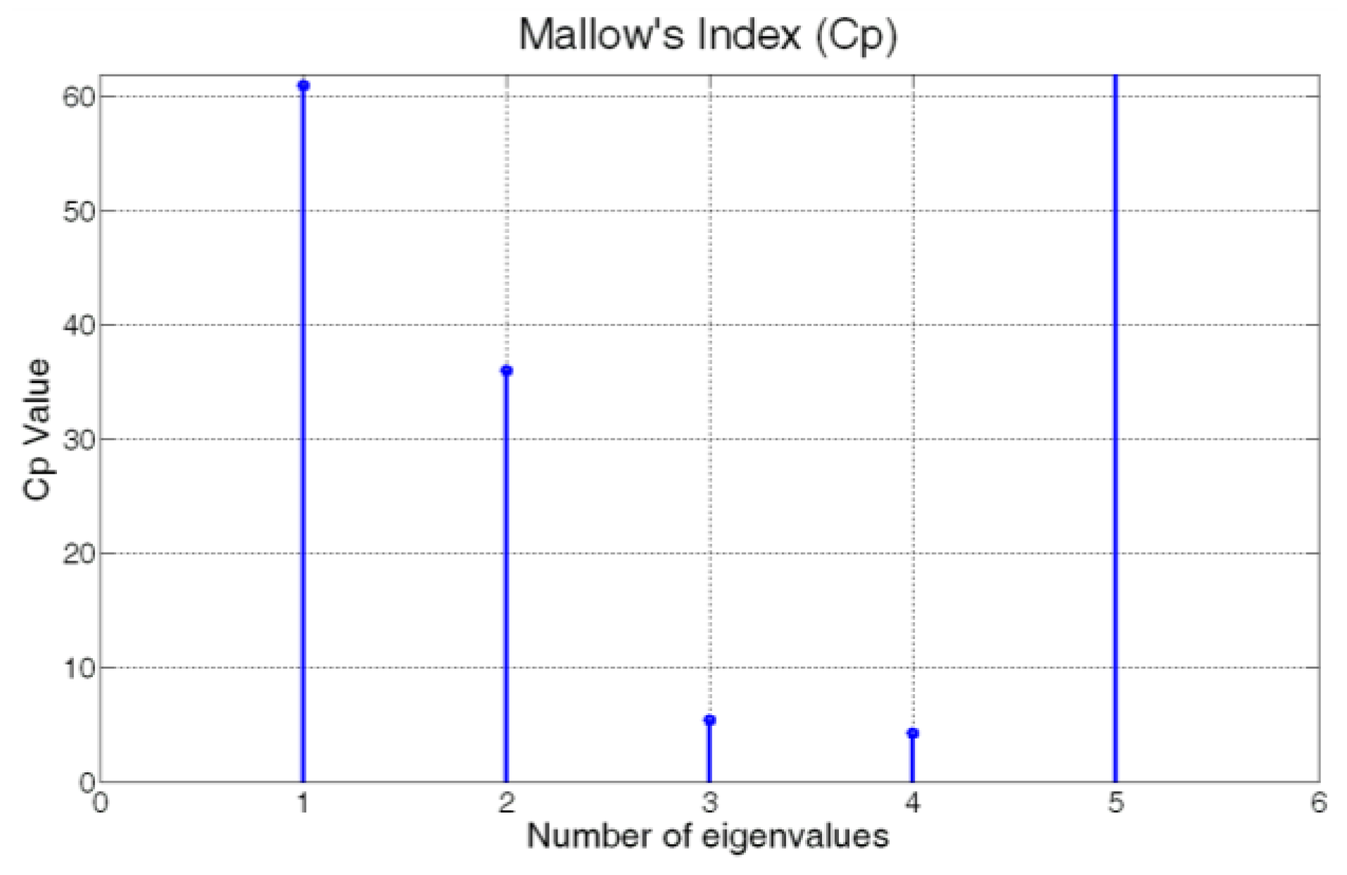
| Number of Eigenvalues | Cp Value |
|---|---|
| 1 | 61.0314 |
| 2 | 35.9931 |
| 3 | 5.3742 |
| 4 | 4.2606 |
| 5 | 1128.8 |
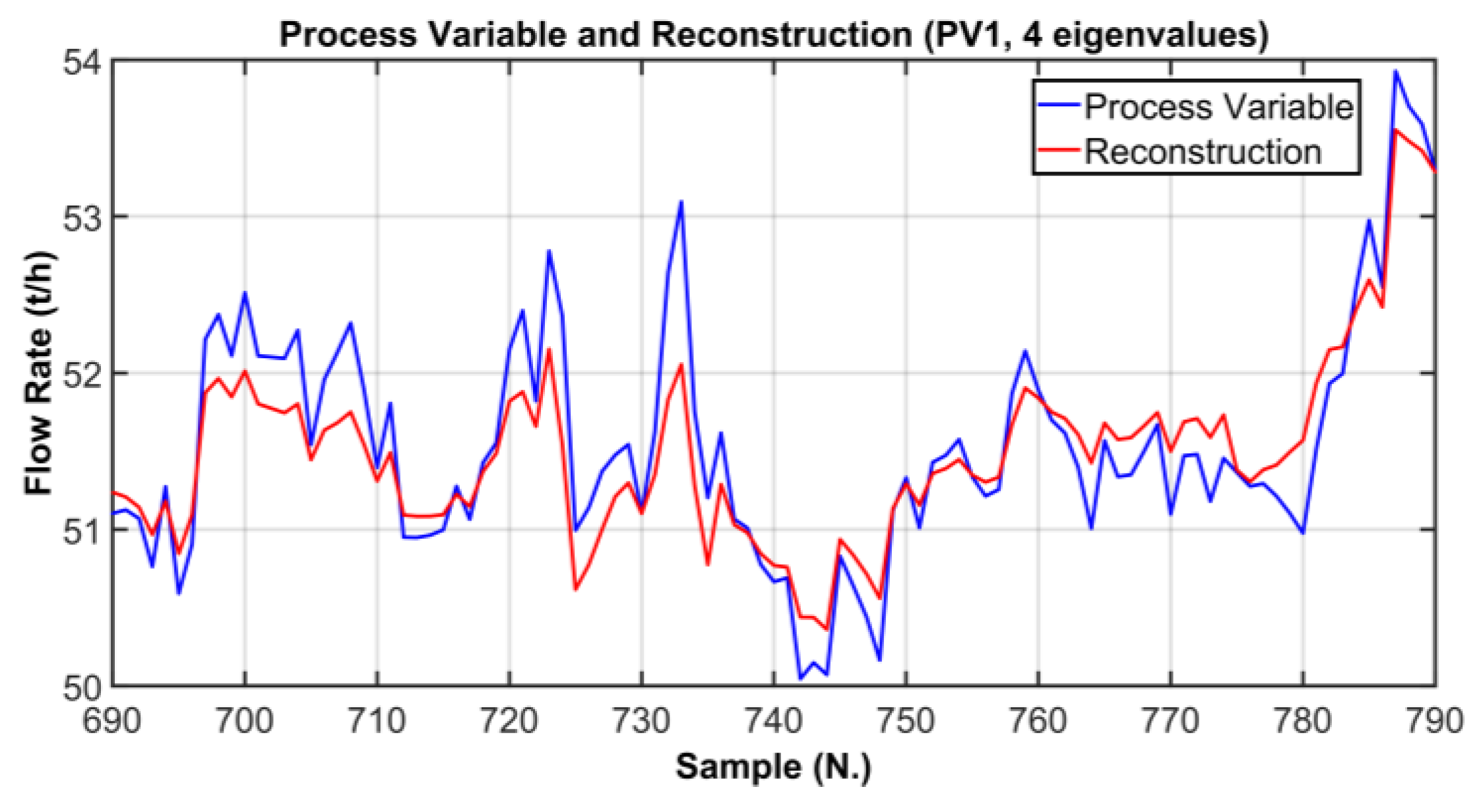
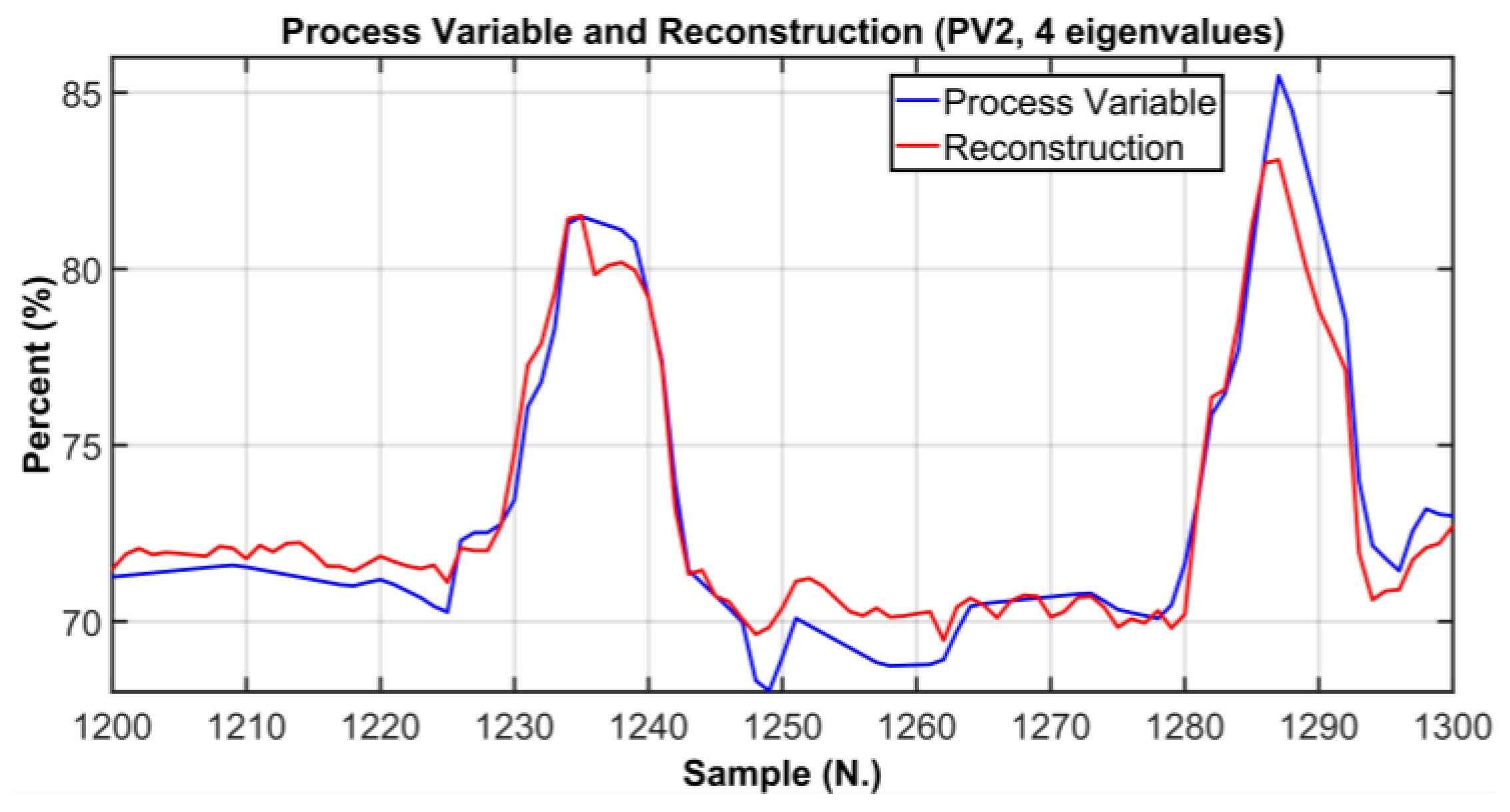
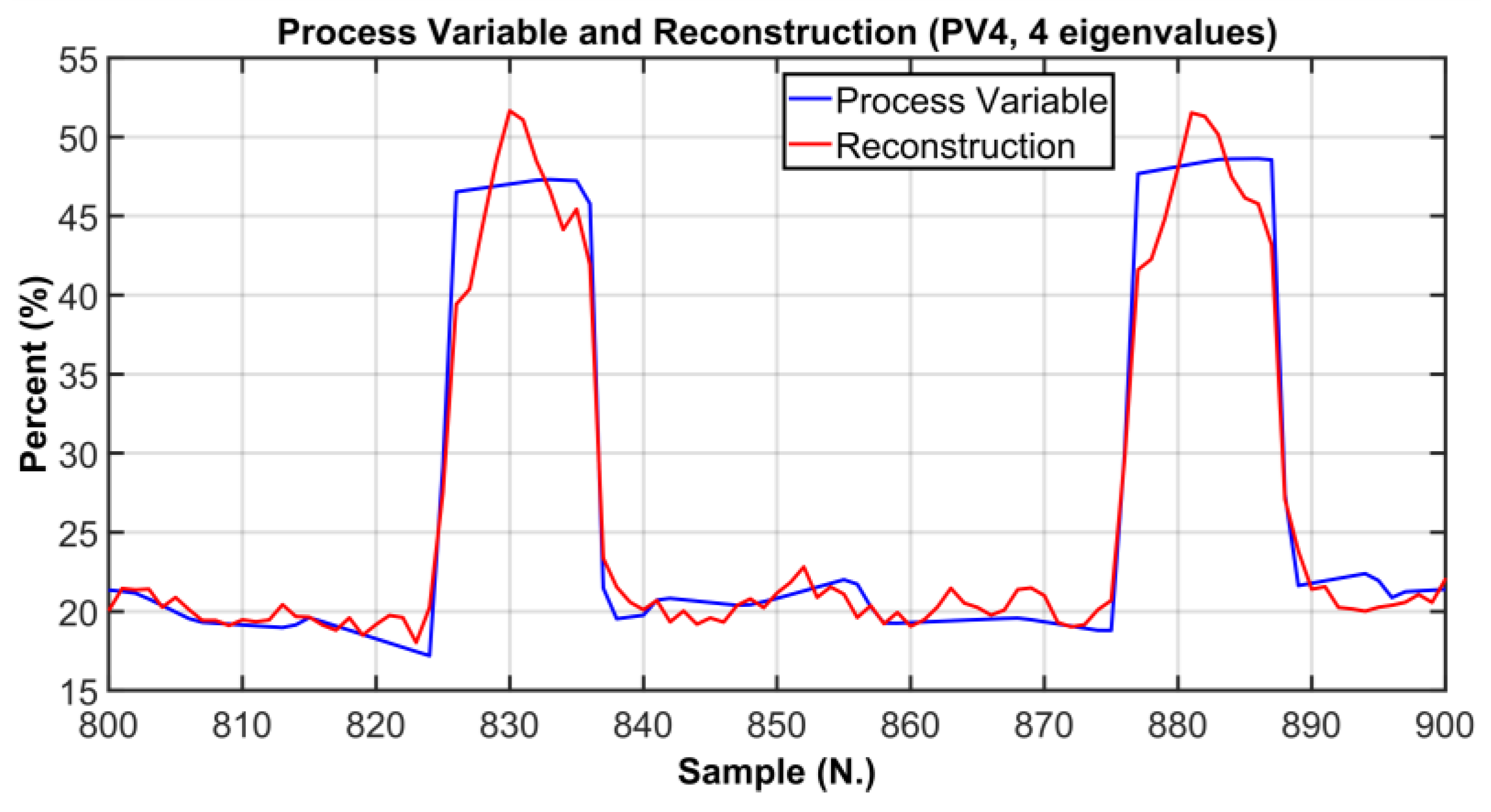
| PV# | RMSE | % RMSE/Range |
|---|---|---|
| PV1 | 0.5148 t/h | 6.8159% |
| PV2 | 4.2280% | 4.7% |
| PV4 | 9.4586% | 10.51% |
| Method | PCs Number |
|---|---|
| AIC | No solution |
| MDL | No solution |
| IEF | No solution |
| PRESScov | No solution |
| RPVcorr | No solution |
| PRESScorr | Ambiguous |
| AC | 1 |
| RPVcov | 3 |
| VRE | 3 |
| ANOVA | 4 |
| AEcorr | 4 |
| PAcorr | 4 |
| CPVcorr | 4 |
| Fault Prototype ID/SPE Component | 1 | 2 | 3 | 4 | 5 | 6 | 7 | 8 | 9 |
|---|---|---|---|---|---|---|---|---|---|
| NOC—ID #1 | 2.49 × 10⁻⁵ | 9.96 × 10⁻⁵ | 1.32 × 10⁻⁵ | 4.87 × 10⁻⁵ | 2.02 × 10⁻⁵ | 1.28 × 10⁻⁵ | 1.42 × 10⁻⁵ | 4.80 × 10⁻⁵ | 9.04 × 10⁻⁶ |
| Fault—ID #2 | 0.49 | 0.99 | 0.29 | 0.36 | 0.42 | 0.27 | 0.33 | 0.45 | 0.18 |
| Fault Prototype ID/SPE Component | 10 | … | 18 | 19 | 20 | 21 | 22 | 23 | … |
| NOC—ID #1 | 0 | … | 9.52 × 10⁻⁵ | 0 | 9.14 × 10⁻⁵ | 9.94 × 10⁻⁵ | 8.51 × 10⁻⁵ | 0 | … |
| Fault—ID #2 | 0.99 | … | 0.98 | 0.99 | 0.98 | 0.99 | 0.97 | 0.99 | … |
| Clusters | JM Distance | Difference | |
|---|---|---|---|
| #1–#2 | 4.59 |  | 0.23 < 0.50 |
| #4–#2 | 4.36 | ||
| #1–#3 | 3.04 | | 0.17 < 0.50 |
| #4–#3 | 2.87 | ||
| #1–#5 | 3.89 | | 0.06 < 0.50 |
| #4–#5 | 3.95 | ||
| Clusters | JM Distance | Difference | |
|---|---|---|---|
| #2–#1 | 4.33 | | 0.17 < 0.50 |
| #4–#1 | 4.16 | ||
| #2–#3 | 3.89 | | 0.14 < 0.50 |
| #4–#3 | 3.75 | ||
| Clusters | JM Distance | Difference | |
|---|---|---|---|
| #1–#2 | 4.53 | | 0.51 > 0.50 |
| #3–#2 | 4.02 | ||
Disclaimer/Publisher’s Note: The statements, opinions and data contained in all publications are solely those of the individual author(s) and contributor(s) and not of MDPI and/or the editor(s). MDPI and/or the editor(s) disclaim responsibility for any injury to people or property resulting from any ideas, methods, instructions or products referred to in the content. |
© 2023 by the authors. Licensee MDPI, Basel, Switzerland. This article is an open access article distributed under the terms and conditions of the Creative Commons Attribution (CC BY) license (https://creativecommons.org/licenses/by/4.0/).
Share and Cite
Zanoli, S.M.; Pepe, C. Design and Implementation of a Fuzzy Classifier for FDI Applied to Industrial Machinery. Sensors 2023, 23, 6954. https://doi.org/10.3390/s23156954
Zanoli SM, Pepe C. Design and Implementation of a Fuzzy Classifier for FDI Applied to Industrial Machinery. Sensors. 2023; 23(15):6954. https://doi.org/10.3390/s23156954
Chicago/Turabian StyleZanoli, Silvia Maria, and Crescenzo Pepe. 2023. "Design and Implementation of a Fuzzy Classifier for FDI Applied to Industrial Machinery" Sensors 23, no. 15: 6954. https://doi.org/10.3390/s23156954