
Thermal Time Constant CNN-Based Spectrometry for Biomedical Applications


Abstract
:1. Introduction
- –
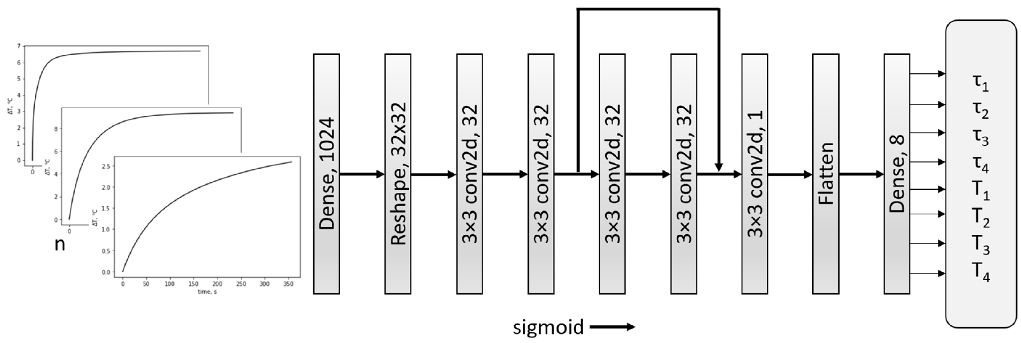
- Section 2: Materials and Methods—presents the proposed approach for the time-constant spectrometry method based on CNN. It includes a description of the proposed structure of the CNN network, the dataset, and the training and validation processes.
- –
- Section 3: Results—is divided into subsections:
- ○
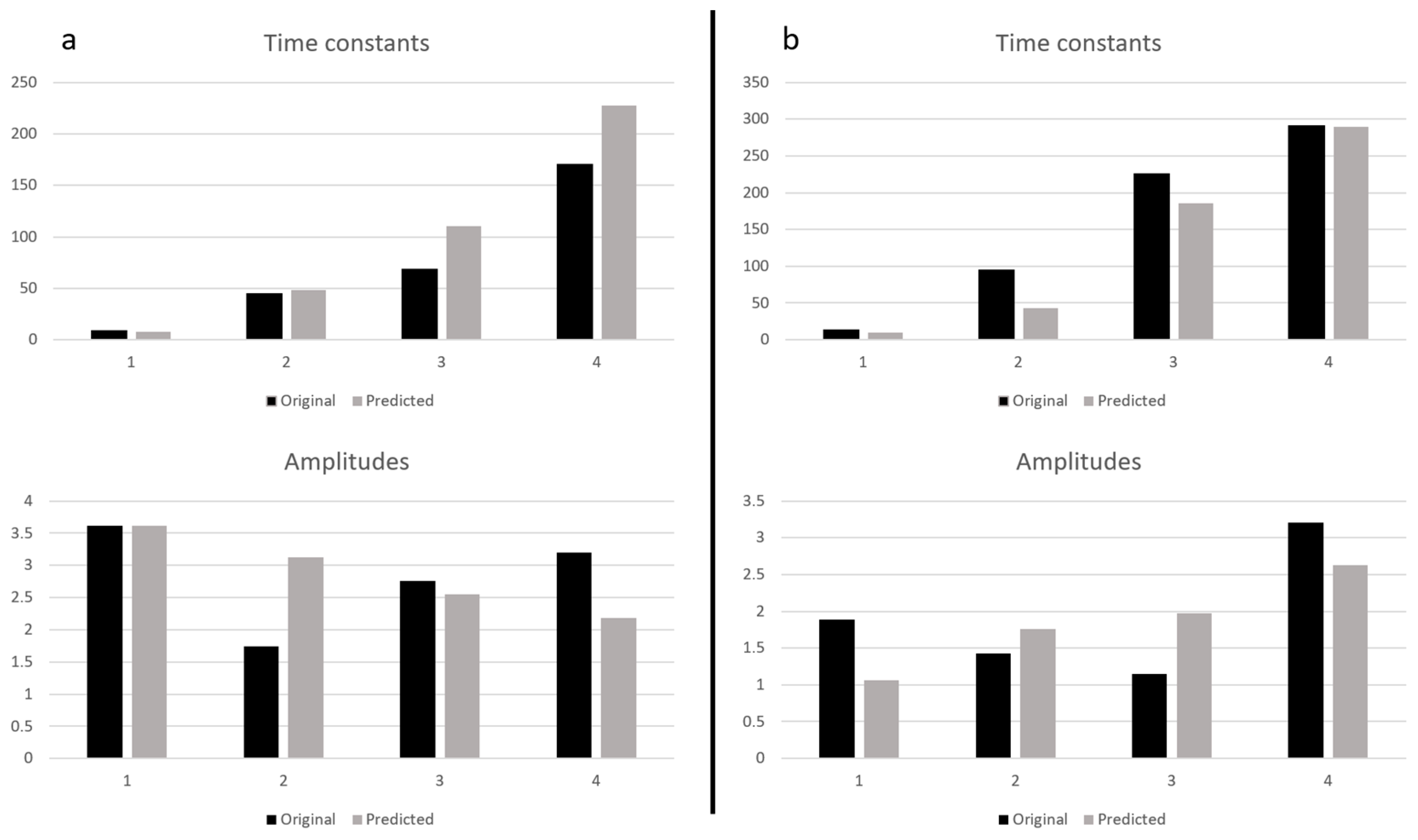
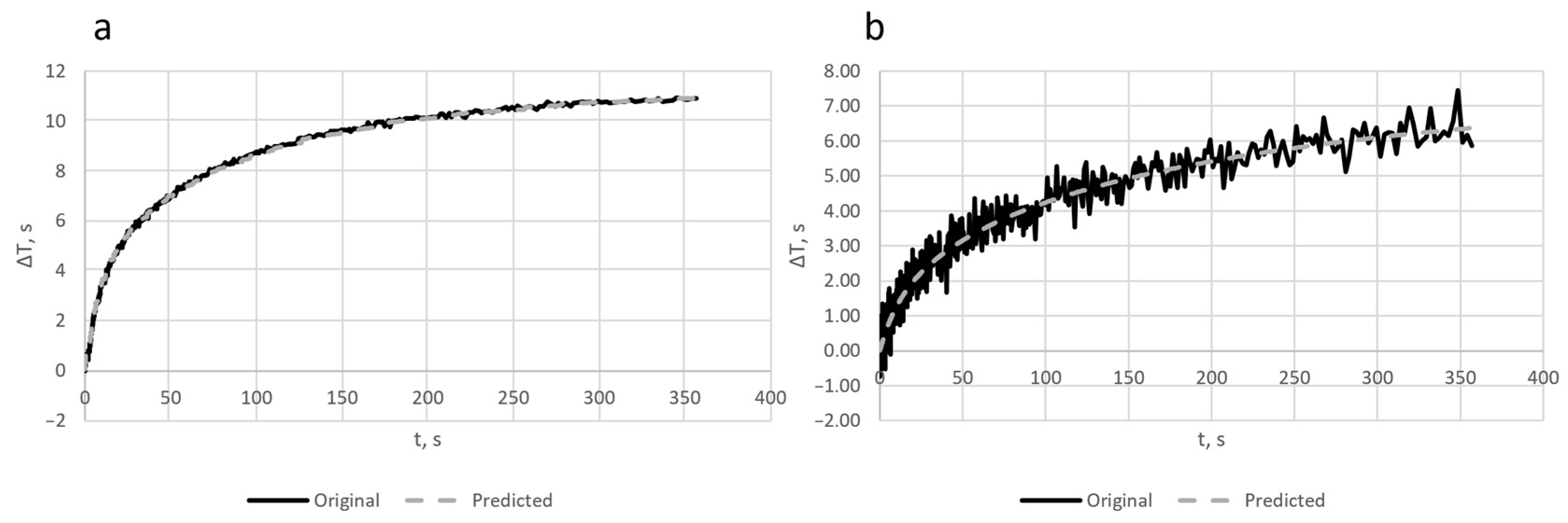
- Section 3.1—presents the results of network validation for artificially generated data.
- ○
- Section 3.2—presents the results for artificially generated data with different levels of noise added.
- ○
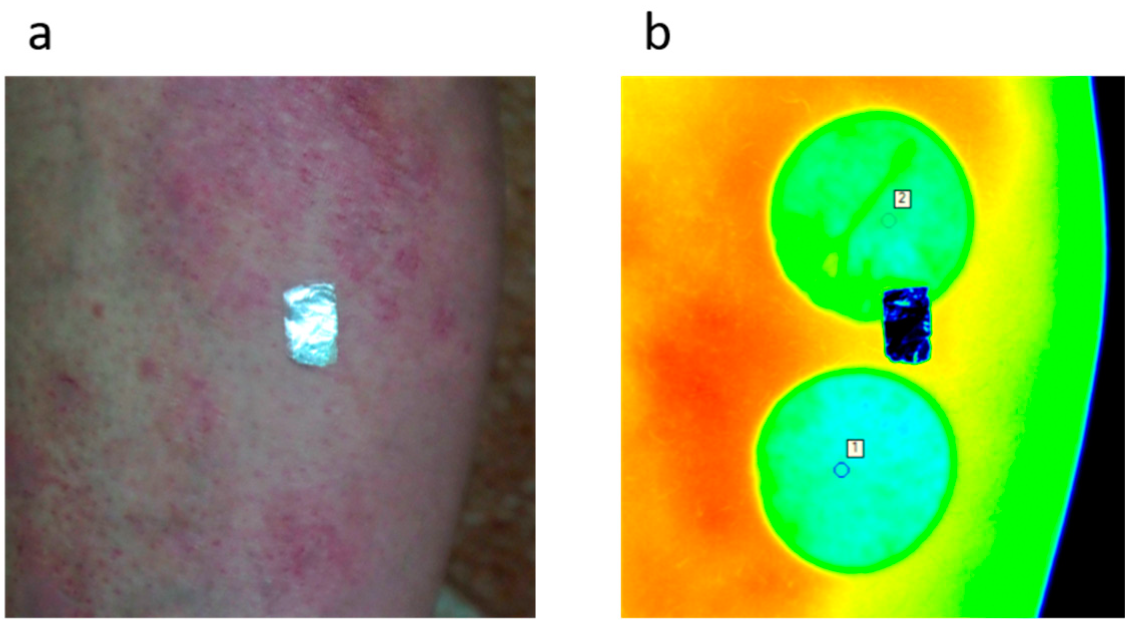
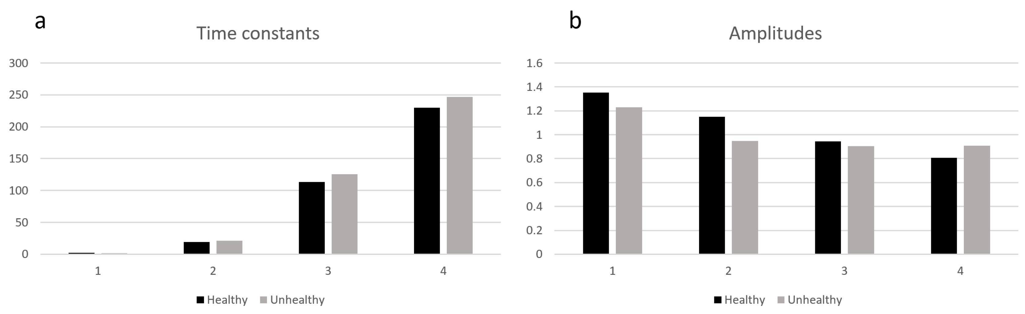
- Section 3.3—presents the network verification for real measurements of the patient suffering from psoriasis—for healthy and unhealthy parts of the skin.
- –
- Section 4—discusses the results, concludes the paper, and lists some possible future work.
2. Materials and Methods
3. Results
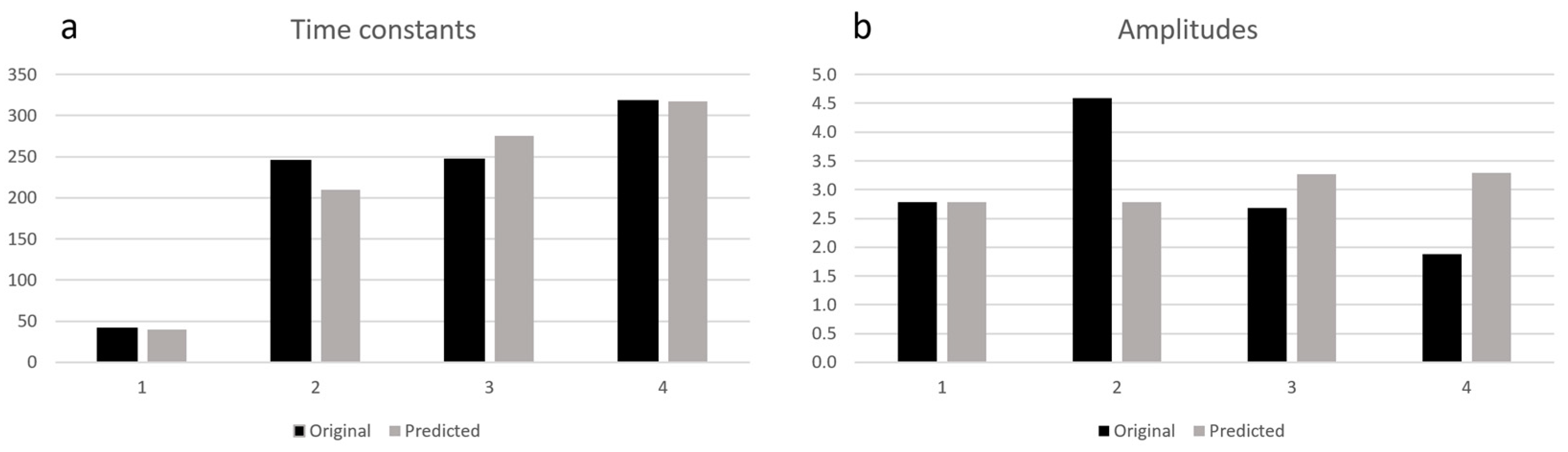
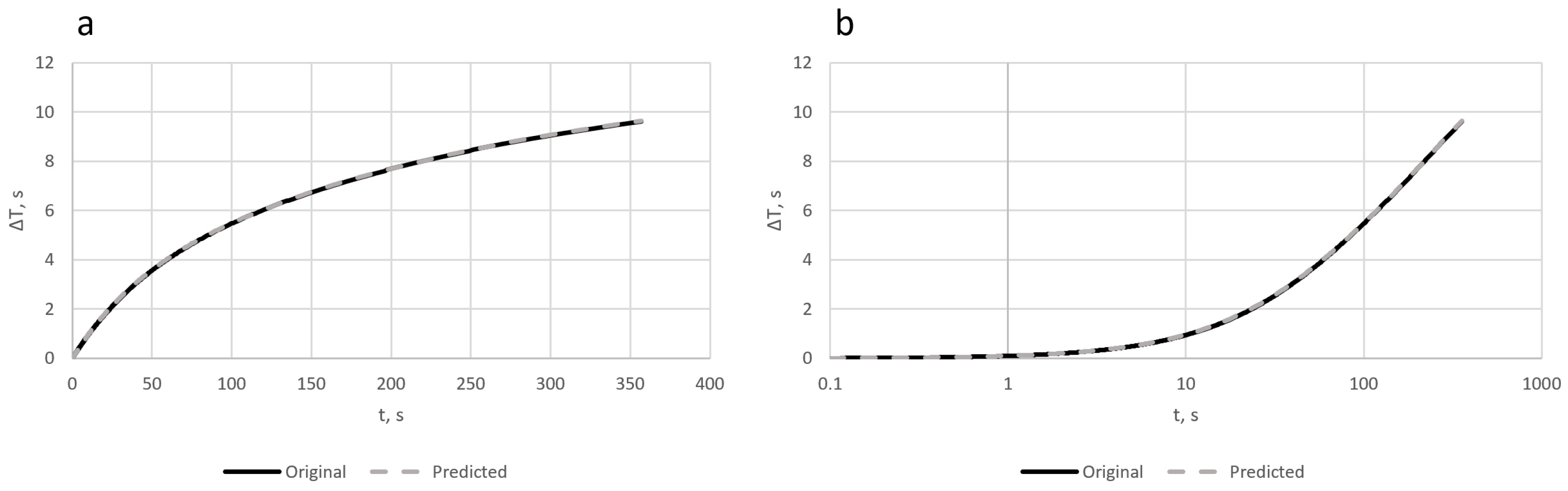
3.1. Network Validation for Artificially Generated Data
3.2. Network Validation for Noisy Data
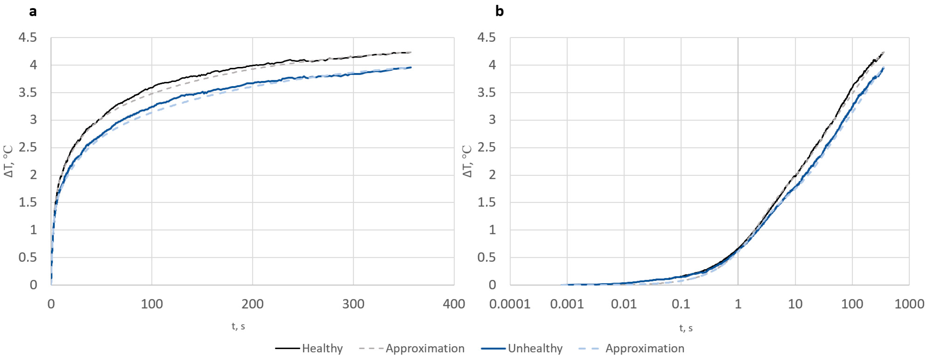
3.3. Results for a Real Data
4. Discussion and Conclusions
Author Contributions
Funding
Institutional Review Board Statement
Informed Consent Statement
Data Availability Statement
Conflicts of Interest
References
- Marco, S.; Palacin, J.; Samitier, J. Improved multiexponential transient spectroscopy by iterative deconvolution. IEEE Trans. Instrum. Meas. 2001, 50, 774–780. [Google Scholar] [CrossRef]
- Garnier, H.; Mensler, M.; Richard, A.A. Continuous-time Model Identification from Sampled Data: Implementation Issues and Performance Evaluation. Int. J. Control 2003, 76, 1337–1357. [Google Scholar] [CrossRef]
- Ljung, L. Experiments with Identification of Continuous-Time Models. In Proceedings of the 15th IFAC Symposium on System Identification, Saint-Malo, France, 6–8 July 2009. [Google Scholar]
- Yarman, B.S.; Kilinc, A.; Aksen, A. Immitance Data Modelling via Linear Interpolation Techniques: A Classical Circuit Theory Approach. Int. J. Circ. Theory Appl. 2004, 32, 1467–1563. [Google Scholar] [CrossRef]
- Jibia, A.U.; Salami, M.J. An Appraisal of Gardner Transform-Based Method of Transient Multiexponential Signal Analysis. Int. J. Comput. Theory Eng. 2012, 4, 16–24. [Google Scholar] [CrossRef]
- De Tommasi, L.; Magnani, A.; De Magistris, M. Advancements in the identification of passive RC networks for compact modeling of thermal effects in electronic devices and systems. Int. J. Numer. Model. 2017, 31, 64–66. [Google Scholar]
- Shindo, Y.; Noro, O. Effective frequency range of ladder network realization for complex permeability of magnetic sheets. IEEJ Trans. Elec. Electron. Eng. 2014, 9, 64–66. [Google Scholar] [CrossRef]
- Wang, K.; Chen, M.Z.Q.; Chen, G. Realization of a transfer function as a passive two-port RC ladder network with a specified gain. Int. J. Circ. Theory. Appl. 2017, 45, 1467–1481. [Google Scholar] [CrossRef]
- Szekely, V. On the representation of infinite-length distributed RC one-ports. IEEE Trans. Circuits Syst. 1991, 38, 711–719. [Google Scholar] [CrossRef]
- Szekely, V. Identification of RC networks by deconvolution: Chances and limits. IEEE Trans. Circuits Syst. 1998, 45, 244–258. [Google Scholar] [CrossRef]
- Vermeersch, B. Thermal AC Modelling, Simulation and Experimental Analysis of Microelectronic Structures including Na-Noscale and High-Speed Effects. Ph.D. Thesis, Gent University, Gent, Belgium, 2009. [Google Scholar]
- Gustavsen, B. Improving the pole relocating properties of vector fitting. IEEE Trans. Power Deliv. 2006, 21, 1587–1592. [Google Scholar] [CrossRef]
- Strakowska, M.; Strąkowski, R.; Strzelecki, M.; De Mey, G.; Wiecek, B. Thermal modelling and screening method for skin pathologies using active thermography. Biocybern. Biomed. Eng. 2018, 38, 602–610. [Google Scholar] [CrossRef]
- Strakowska, M.; Chatzipanagiotou, P.; De Mey, M.; Chatziathanasiou, V.; Wiecek, B. Novel software for medical and technical Object Identification (TOI) using dynamic temperature measurements by fast IR cameras. In Proceedings of the 14th Quantitative Infra-Red Thermography Conference, Berlin, Germany, 25–29 June 2018; Volume 38, pp. 602–610. [Google Scholar]
- Chatzipanagiotou, P.; Chatziathanasiou, V.; Papagiannopoulos, I.; De Mey, G.; Wiecek, B. Dynamic thermal analysis of underground medium power cables using thermal impedance, time constant distribution and structure function. Appl. Therm. Eng. 2013, 60, 256–260. [Google Scholar]
- Chatzipanagiotou, P.; Strąkowska, M.; De Mey, G.; Więcek, B. A new software tool for transient thermal analysis based on fast IR camera temperature measurement. Meas. Autom. Monit. 2013, 63, 49–51. [Google Scholar]
- CAPTAIN-Computer-AidedProgramforTime-SeriesAnalysisandIdentificationofNoisySystems. Available online: http://www.es.lancs.ac.uk/cres/captain/ (accessed on 30 June 2023).
- Karimifard, P.; Gharehpetian, G.B.; Tenbohlen, S. Localization of winding radial deformation and determination of deformation extent using vector fitting-based estimated transfer function. Euro. Trans. Electr. Power 2013, 19, 749–762. [Google Scholar] [CrossRef]
- Strakowska, M.; Chatzipanagiotou, P.; De Mey, G.; Chatziathanasiou, V.; Więcek, B. Multilayer thermal object identification in frequency domain using IR thermography and vector fitting. Int. J. Circuit. Theory Appl. 2020, 48, 1523–1533. [Google Scholar] [CrossRef]
- Gupta, J.; Pathak, S.; Kumar, G. Deep Learning (CNN) and Transfer Learning: A Review. J. Phys. Conf. Ser. 2022, 2273, 012029. [Google Scholar] [CrossRef]
- Kim, J.-H.; Lee, J.-S. Deep Residual Network with Enhanced Upscaling Module for Super-Resolution. In Proceedings of the IEEE Conference on Computer Vision and Pattern Recognition (CVPR) Workshops, Salt-Lake City, UT, USA, 18–22 June 2018; pp. 800–808. [Google Scholar]
- Li, J.; Fang, F.; Mei, K.; Zhang, G. Multi-scale Residual Network for Image Super-Resolution. In Proceedings of the 15th European Conference on Computer Vision, Munich, Germany, 8–14 September 2018. [Google Scholar]
- Bengio, Y.; Simard, P.; Frasconi, P. Learning long-term dependencies with gradient descent is difficult. IEEE Trans. Neural Netw. 1994, 5, 157–166. [Google Scholar] [CrossRef]
- Glorot, X.; Bengio, Y. Understanding the difficulty of training deep feedforward neural networks. In Proceedings of the Thirteenth International Conference on Artificial Intelligence and Statistics, Sardinia, Italy, 13–15 May 2010. [Google Scholar]
- Ioffe, S.; Szegedy, C. Batch normalization: Accelerating deep network training by reducing internal covariate shift. In Proceedings of the 32nd International Conference on International Conference on Machine Learning, Lille, France, 6–11 July 2015. [Google Scholar]
- Ornek, A.H.; Ceylan, M. CodCAM: A new ensemble visual explanation for classification of medical thermal images. Quant. InfraRed Thermogr. J. 2023, 1–25. [Google Scholar] [CrossRef]
- Özdil, A.; Yilmaz, B. Medical infrared thermal image based fatty liver classification using machine and deep learning. Quant. InfraRed Thermogr. J. 2023, 1–18. [Google Scholar] [CrossRef]
- Mahoro, E.; Akhloufi, M. A Breast cancer classification on thermograms using deep CNN and transformers. Quant. InfraRed Thermogr. J. 2022, 1–20. [Google Scholar] [CrossRef]
- Bardhan, S.; Nath, S.; Debnath, T.; Bhattacharjee, D.; Bhowmik, M.K. Designing of an inflammatory knee joint thermogram dataset for arthritis classification using deep convolution neural network. Quant. InfraRed Thermogr. J. 2022, 19, 145–171. [Google Scholar] [CrossRef]
- Kaczmarek, M.; Nowakowski, A. Active IR-Thermal Imaging in Medicine. J. Nondestruct. Eval. 2016, 35, 19. [Google Scholar] [CrossRef] [Green Version]
- Available online: https://www.tensorflow.org/guide/keras?hl=pl (accessed on 11 July 2023).
- Ring, E.F.J.; Ammer, K. The Technique of InfraRed Imaging in Medicine. Thermol. Int. 2000, 10, 7–14. [Google Scholar]
- Machado, Á.S.; Cañada-Soriano, M.; Jimenez-Perez, I.; Gil-Calvo, M.; Pivetta Carpes, F.; Perez-Soriano, P.; Ignacio Priego-Quesada, J. Distance and camera features measurements affect the detection of temperature asymmetries using infrared thermography. Quant. InfraRed Thermogr. J. 2022, 1–13. [Google Scholar] [CrossRef]
- Lagarias, J.C.; Reeds, J.A.; Wright, M.H.; Wright, P.E. Convergence Properties of the Nelder-Mead Simplex Method in Low Dimensions. SIAM J. Optim. 1998, 9, 112–147. [Google Scholar] [CrossRef] [Green Version]
- Krichen, M.; Mihoub, A.; Alzahrani, M.Y.; Adoni, W.Y.H.; Nahhal, T. Are Formal Methods Applicable to Machine Learning And Artificial Intelligence? In Proceedings of the 2022 2nd International Conference of Smart Systems and Emerging Technologies (SMARTTECH), Riyadh, Saudi Arabia, 9–11 May 2022; pp. 48–53. [Google Scholar]
- Gehr, T.; Mirman, M.; Drachsler-Cohen, D.; Tsankov, P.; Chaudhuri, S.; Vechev, M. Ai2: Safety and robustness certification of neural networks with abstract interpretation. In Proceedings of the 2018 IEEE Symposium on Security and Privacy (SP), San Francisco, CA, USA, 20–24 May 2018; pp. 3–18. [Google Scholar]
- Singh, G.; Gehr, T.; Mirman, M.; Puschel, M.; Vechev, M.T. Fast and effective robustness certification. NeurIPS 2018, 1, 6. [Google Scholar]
- Singh, G.; Gehr, T.; Puschel, M.; Vechev, M. An abstract domain for certifying neural networks. Proc. ACM Program. Lang. 2019, 3, 1–30. [Google Scholar] [CrossRef] [Green Version]


| Parameter | Values/Method |
|---|---|
| Exponential parts | 4 |
| τi range | (0–1) s |
| Ti range | (0–1) °C |
| Train dataset/epoch | 10,000 |
| Validation data | 1000 |
| Optimizer | Stochastic Gradient Decent |
| Loss Function | 0.2·mse(τ) + 0.8·mse(T) |
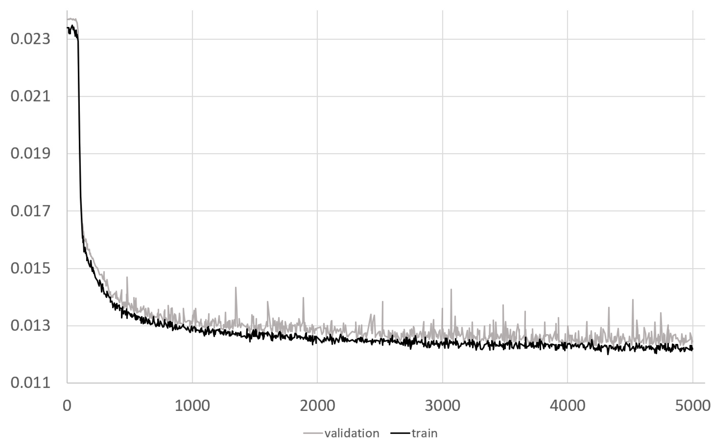
| Epoch no. | 5000 |
| Activation function | sigmoid |
| Component No. | τi | Ti | T(t) |
|---|---|---|---|
| 1 | 0.00128 | 0.03642 | 0.01353 |
| 2 | 0.01022 | 0.05394 | |
| 3 | 0.01336 | 0.0555 | |
| 4 | 0.01327 | 0.05225 | |
| mean | 0.00953 | 0.04952 |
| Noise Variance | i | τi | Ti | T(t) |
|---|---|---|---|---|
| 0.0001 | 1 | 0.00179 | 0.03289 | 0.01180 |
| 2 | 0.01010 | 0.05359 | ||
| 3 | 0.01468 | 0.05708 | ||
| 4 | 0.01615 | 0.04853 | ||
| mean | 0.01068 | 0.04802 | ||
| 0.0005 | 1 | 0.00391 | 0.04794 | 0.01261 |
| 2 | 0.01459 | 0.06010 | ||
| 3 | 0.02036 | 0.05894 | ||
| 4 | 0.02189 | 0.05778 | ||
| mean | 0.01518 | 0.05619 | ||
| 0.001 | 1 | 0.00707 | 0.06066 | 0.02051 |
| 2 | 0.01524 | 0.06194 | ||
| 3 | 0.02753 | 0.05982 | ||
| 4 | 0.03403 | 0.06350 | ||
| mean | 0.02096 | 0.06148 | ||
| 0.0015 | 1 | 0.00930 | 0.06405 | 0.01909 |
| 2 | 0.01818 | 0.06456 | ||
| 3 | 0.03471 | 0.06316 | ||
| 4 | 0.03842 | 0.06611 | ||
| mean | 0.02515 | 0.06447 | ||
| 0.0025 | 1 | 0.00948 | 0.07460 | 0.03609 |
| 2 | 0.02351 | 0.06238 | ||
| 3 | 0.04262 | 0.06651 | ||
| 4 | 0.06015 | 0.07994 | ||
| mean | 0.03394 | 0.07085 | ||
| 0.005 | 1 | 0.01724 | 0.09785 | 0.04929 |
| 2 | 0.02643 | 0.06824 | ||
| 3 | 0.05885 | 0.07596 | ||
| 4 | 0.08743 | 0.07964 | ||
| mean | 0.04748 | 0.08782 |
| Case | τi | Ti |
|---|---|---|
| Healthy | 1.9486818 | 1.354312 |
| 18.936752 | 1.1490566 | |
| 113.21907 | 0.9453574 | |
| 230.25365 | 0.8074841 | |
| Unhealthy | 1.7264072 | 1.231425 |
| 21.461962 | 0.9482369 | |
| 125.83128 | 0.902929 | |
| 246.69447 | 0.9088539 |
Disclaimer/Publisher’s Note: The statements, opinions and data contained in all publications are solely those of the individual author(s) and contributor(s) and not of MDPI and/or the editor(s). MDPI and/or the editor(s) disclaim responsibility for any injury to people or property resulting from any ideas, methods, instructions or products referred to in the content. |
© 2023 by the authors. Licensee MDPI, Basel, Switzerland. This article is an open access article distributed under the terms and conditions of the Creative Commons Attribution (CC BY) license (https://creativecommons.org/licenses/by/4.0/).
Share and Cite
Strąkowska, M.; Strzelecki, M. Thermal Time Constant CNN-Based Spectrometry for Biomedical Applications. Sensors 2023, 23, 6658. https://doi.org/10.3390/s23156658
Strąkowska M, Strzelecki M. Thermal Time Constant CNN-Based Spectrometry for Biomedical Applications. Sensors. 2023; 23(15):6658. https://doi.org/10.3390/s23156658
Chicago/Turabian StyleStrąkowska, Maria, and Michał Strzelecki. 2023. "Thermal Time Constant CNN-Based Spectrometry for Biomedical Applications" Sensors 23, no. 15: 6658. https://doi.org/10.3390/s23156658