
MFF-YOLO: An Accurate Model for Detecting Tunnel Defects Based on Multi-Scale Feature Fusion

Abstract
:1. Introduction
2. Related Work
2.1. Convolutional Neural Network
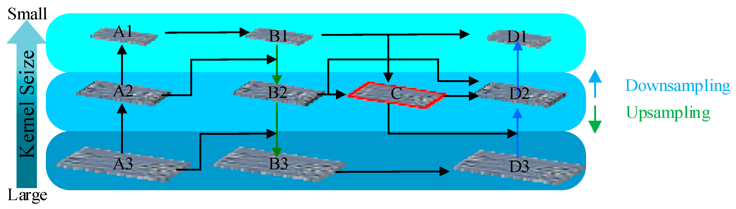
2.2. Multi-Scale Feature Fusion
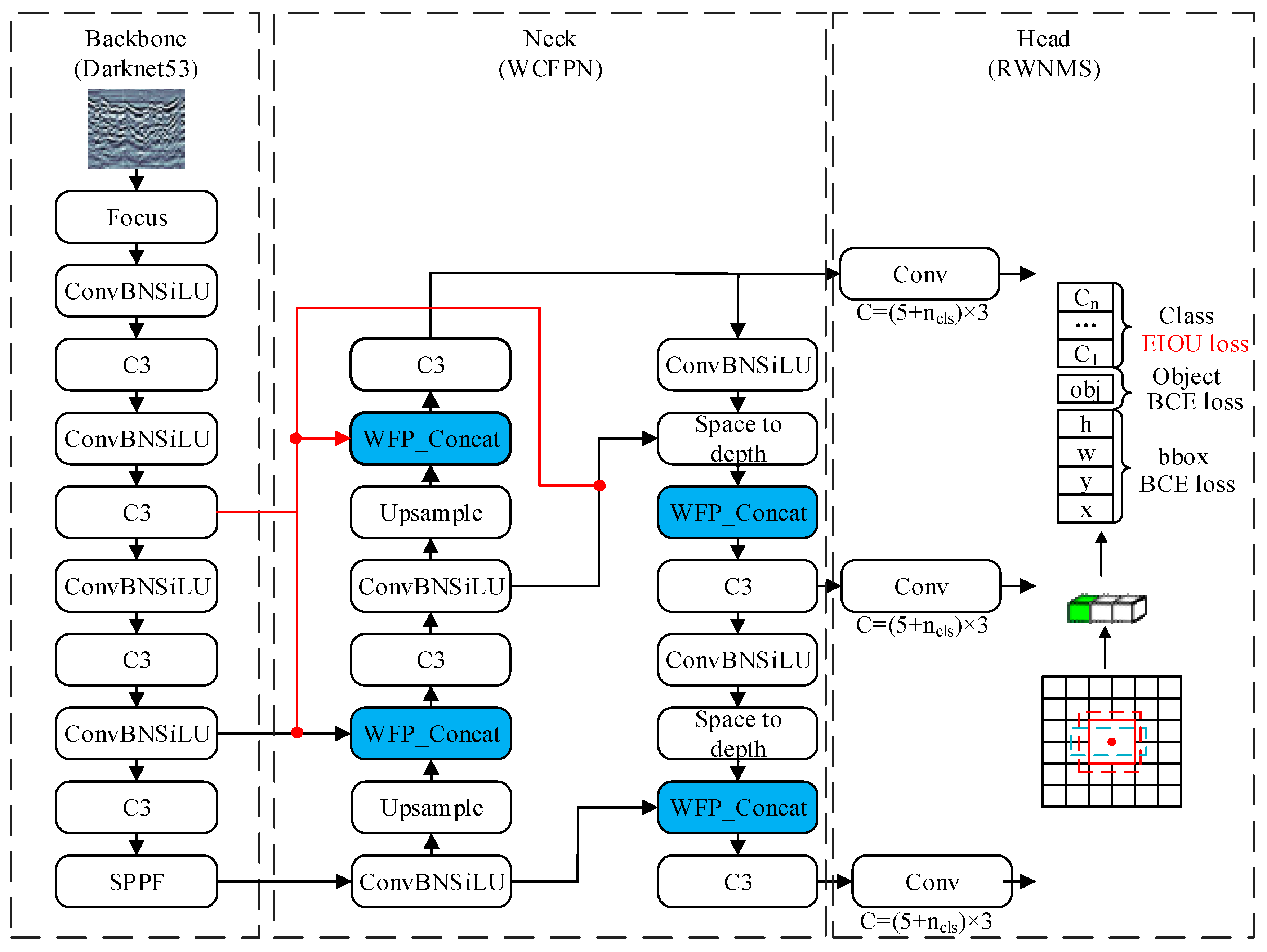
3. Methods
3.1. WCFPN
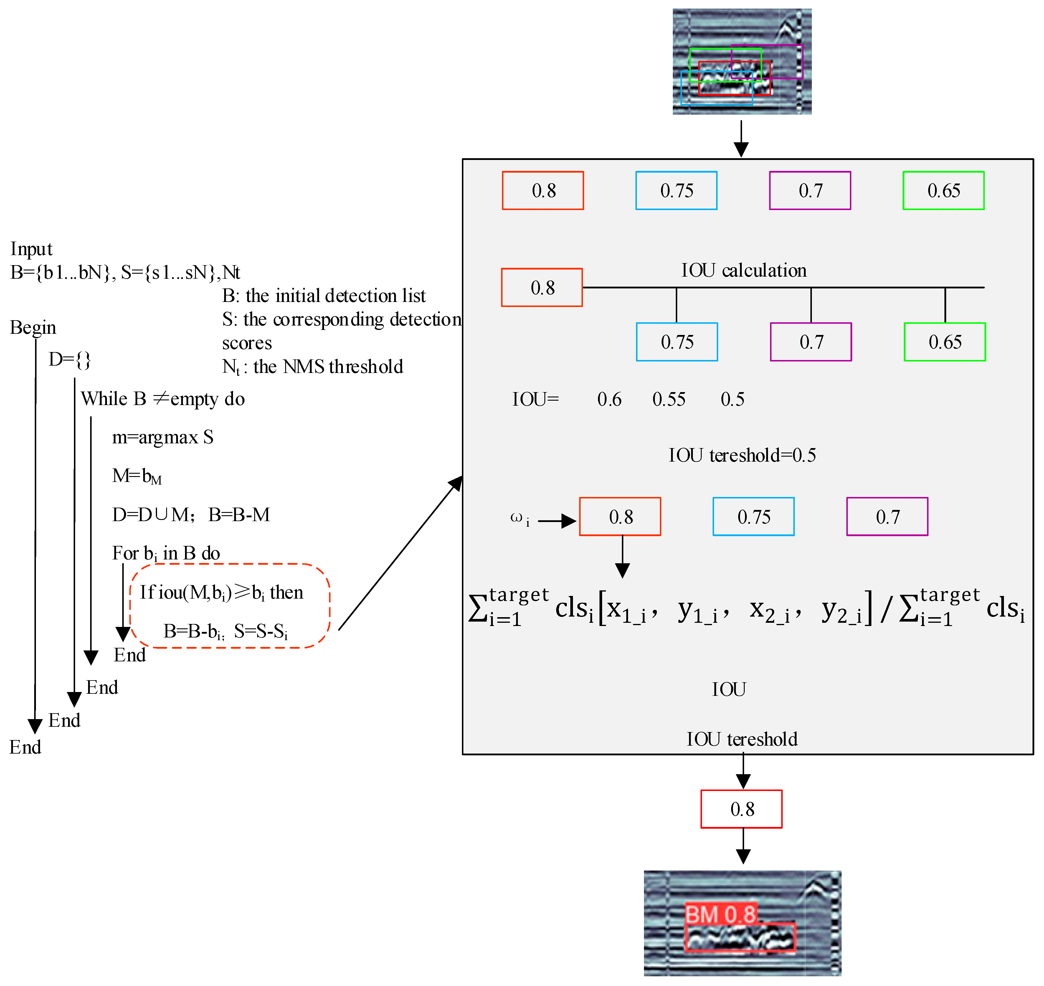
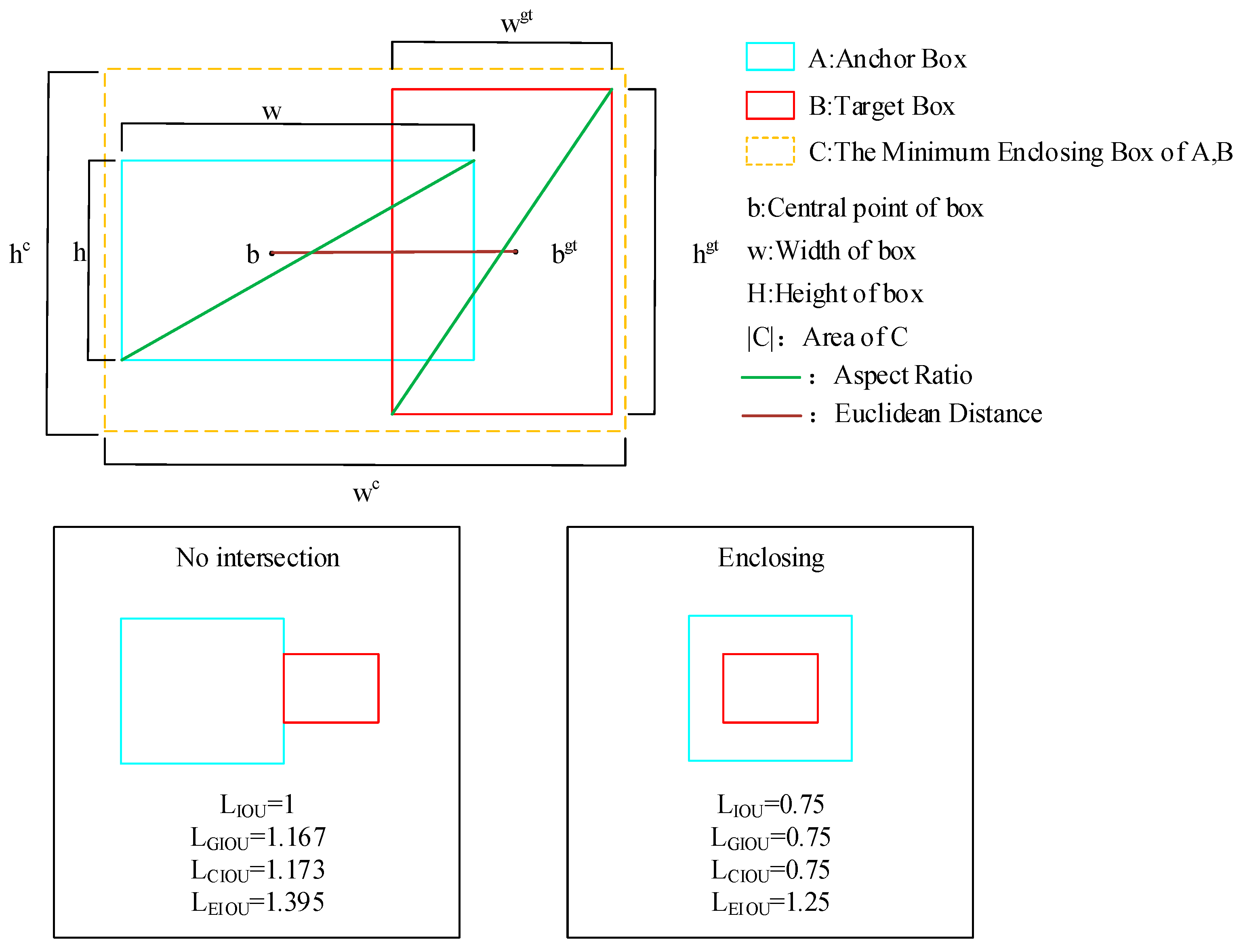
3.2. RWNMS
4. Experimental Studies
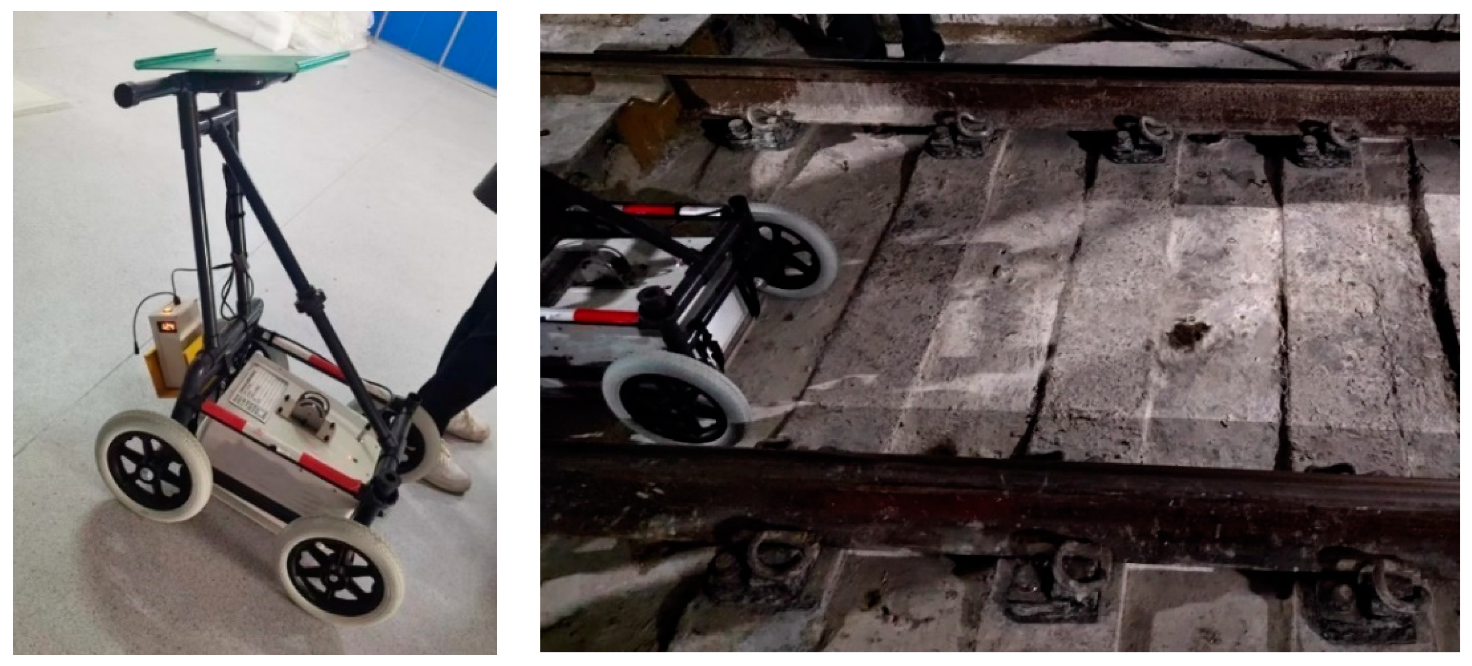
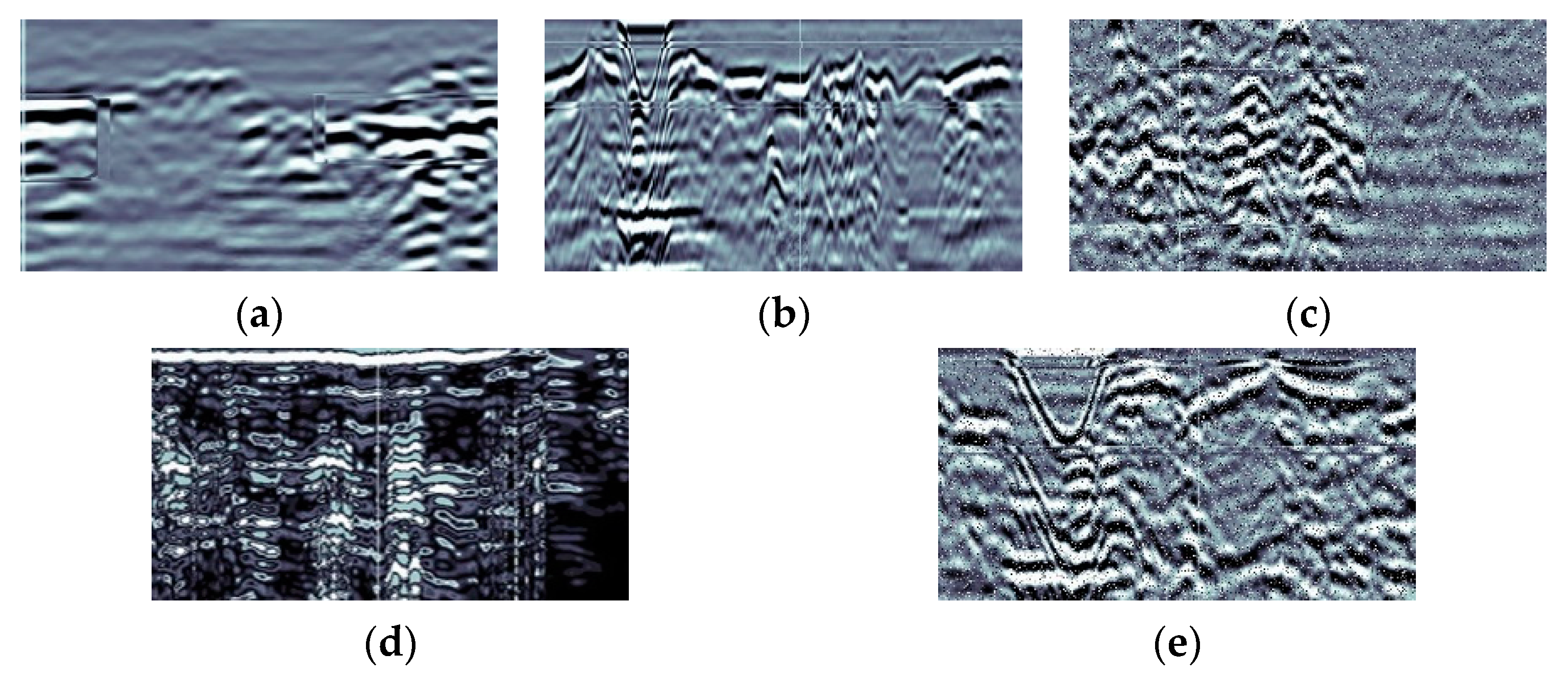
4.1. Data Processing
4.2. Experimental Procedure
4.2.1. Experimental Configuration
4.2.2. Evaluation Indicators
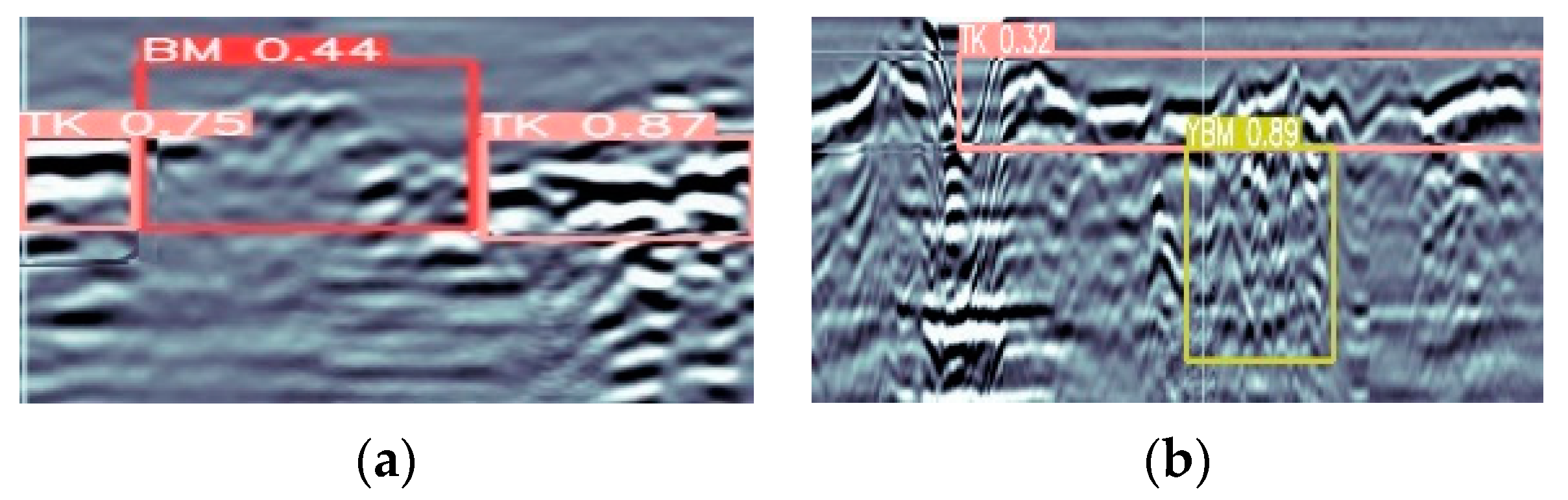
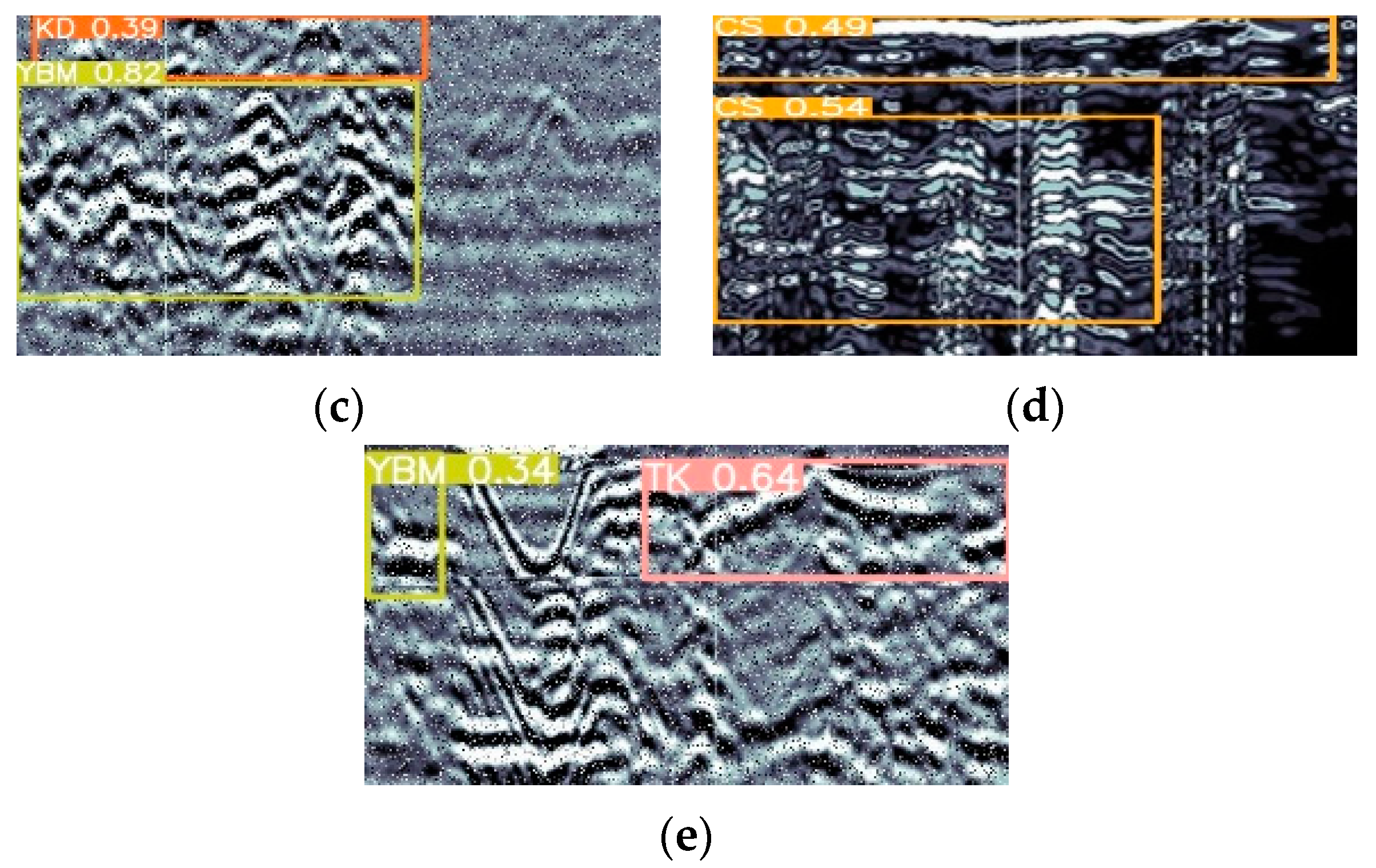
5. Results
6. Conclusions
Author Contributions
Funding
Data Availability Statement
Conflicts of Interest
References
- Wang, J.; Xie, X.; Huang, H. A fuzzy comprehensive evaluation system of mountain tunnel lining based on the fast nondestructive inspection. In Proceedings of the 2011 International Conference on Remote Sensing, Environment and Transportation Engineering, Nanjing, China, 24–26 June 2011; pp. 2832–2834. [Google Scholar]
- Ni, Y.; Mao, J.; Fu, Y.; Wang, H.; Zong, H.; Luo, K. Damage Detection and Localization of Bridge Deck Pavement Based on Deep Learning. Sensors 2023, 23, 5138. [Google Scholar] [CrossRef] [PubMed]
- Kao, S.-P.; Chang, Y.-C.; Wang, F.-L. Combining the YOLOv4 Deep Learning Model with UAV Imagery Processing Technology in the Extraction and Quantization of Cracks in Bridges. Sensors 2023, 23, 2572. [Google Scholar] [CrossRef]
- Santaniello, P.; Russo, P. Bridge Damage Identification Using Deep Neural Networks on Time–Frequency Signals Representation. Sensors 2023, 23, 6152. [Google Scholar] [CrossRef] [PubMed]
- Yan, R.; Zhang, R.; Bai, J.; Hao, H.; Guo, W.; Gu, X.; Liu, Q. STMS-YOLOv5: A Lightweight Algorithm for Gear Surface Defect Detection. Sensors 2023, 23, 5992. [Google Scholar] [CrossRef] [PubMed]
- Guo, Z.; Wang, C.; Yang, G.; Huang, Z.; Li, G. MSFT-YOLO: Improved YOLOv5 Based on Transformer for Detecting Defects of Steel Surface. Sensors 2022, 22, 3467. [Google Scholar] [CrossRef] [PubMed]
- Shaikh, K.; Hussain, I.; Chowdhry, B.S. Wheel Defect Detection Using a Hybrid Deep Learning Approach. Sensors 2023, 23, 6248. [Google Scholar] [CrossRef]
- Sjölander, A.; Belloni, V.; Ansell, A.; Nordström, E. Towards automated inspections of tunnels: A review of optical inspections and autonomous assessment of concrete tunnel linings. Sensors 2023, 23, 3189. [Google Scholar] [CrossRef]
- Maeda, K.; Takada, S.; Haruyama, T.; Togo, R.; Ogawa, T.; Haseyama, M. Distress Detection in Subway Tunnel Images via Data Augmentation Based on Selective Image Cropping and Patching. Sensors 2022, 22, 8932. [Google Scholar] [CrossRef]
- Lei, Y.; Jiang, B.; Su, G.; Zou, Y.; Qi, F.; Li, B.; Jia, F.; Tian, T.; Qu, Q. Application of Air-Coupled Ground Penetrating Radar Based on FK Filtering and BP Migration in High-Speed Railway Tunnel Detection. Sensors 2023, 23, 4343. [Google Scholar] [CrossRef]
- Wu, X.; Bao, X.; Shen, J.; Chen, X.; Cui, H. Evaluation of Void Defects behind Tunnel Lining through GPR forward Simulation. Sensors 2022, 22, 9702. [Google Scholar] [CrossRef]
- Ali, L.; Alnajjar, F.; Jassmi, H.A.; Gocho, M.; Khan, W.; Serhani, M.A. Performance evaluation of deep CNN-based crack detection and localization techniques for concrete structures. Sensors 2021, 21, 1688. [Google Scholar] [CrossRef]
- Wang, A.; Togo, R.; Ogawa, T.; Haseyama, M. Defect detection of subway tunnels using advanced U-Net network. Sensors 2022, 22, 2330. [Google Scholar] [CrossRef]
- Li, G.; Ma, B.; He, S.; Ren, X.; Liu, Q. Automatic tunnel crack detection based on u-net and a convolutional neural network with alternately updated clique. Sensors 2020, 20, 717. [Google Scholar] [CrossRef] [Green Version]
- Zhu, A.; Chen, S.; Lu, F.; Ma, C.; Zhang, F. Recognition Method of Tunnel Lining Defects Based on Deep Learning. Wirel. Commun. Mob. Comput. 2021, 2021, 9070182. [Google Scholar] [CrossRef]
- Zhu, A.; Ma, C.; Chen, S.; Wang, B.; Guo, H. Tunnel Lining Defect Identification Method Based on Small Sample Learning. Wirel. Commun. Mob. Comput. 2022, 2022, 1096467. [Google Scholar] [CrossRef]
- Krizhevsky, A.; Sutskever, I.; Hinton, G.E. Imagenet classification with deep convolutional neural networks. Commun. ACM 2017, 60, 84–90. [Google Scholar] [CrossRef] [Green Version]
- Girshick, R.; Donahue, J.; Darrell, T.; Malik, J. Rich feature hierarchies for accurate object detection and semantic segmentation. In Proceedings of the IEEE Conference on Computer Vision and Pattern Recognition, Columbus, OH, USA, 23–28 June 2014; pp. 580–587. [Google Scholar]
- Cai, Z.; Vasconcelos, N. Cascade r-cnn: Delving into high quality object detection. In Proceedings of the IEEE Conference on Computer Vision and Pattern Recognition, Salt Lake City, UT, USA, 18–23 June 2018; pp. 6154–6162. [Google Scholar]
- Ren, S.; He, K.; Girshick, R.; Sun, J. Faster r-cnn: Towards real-time object detection with region proposal networks. Adv. Neural Inf. Process. Syst. 2015, 1137–1149. [Google Scholar] [CrossRef] [Green Version]
- Srinivasu, P.N.; SivaSai, J.G.; Ijaz, M.F.; Bhoi, A.K.; Kim, W.; Kang, J.J. Classification of skin disease using deep learning neural networks with MobileNet V2 and LSTM. Sensors 2021, 21, 2852. [Google Scholar] [CrossRef]
- Xu, X.; Zhao, M.; Shi, P.; Ren, R.; He, X.; Wei, X.; Yang, H. Crack detection and comparison study based on faster R-CNN and mask R-CNN. Sensors 2022, 22, 1215. [Google Scholar] [CrossRef] [PubMed]
- Liu, W.; Anguelov, D.; Erhan, D.; Szegedy, C.; Reed, S.; Fu, C.Y.; Berg, A.C. Ssd: Single shot multibox detector. In Proceedings of the Computer Vision–ECCV 2016: 14th European Conference, Amsterdam, The Netherlands, 11–14 October 2016; pp. 21–37. [Google Scholar]
- Fu, C.Y.; Liu, W.; Ranga, A.; Tyagi, A.; Berg, A.C. Dssd: Deconvolutional single shot detector. arXiv 2017, arXiv:1701.06659. [Google Scholar]
- Li, Z.; Zhou, F. FSSD: Feature fusion single shot multibox detector. arXiv 2017, arXiv:1712.00960. [Google Scholar]
- Liu, S.; Huang, D. Receptive field block net for accurate and fast object detection. In Proceedings of the European conference on computer vision (ECCV), Tel Aviv, Israel, 23–27 October 2022; pp. 385–400. [Google Scholar]
- Zhang, S.; Wen, L.; Bian, X.; Lei, Z.; Li, S.Z. Single-shot refinement neural network for object detection. In Proceedings of the IEEE Conference on Computer Vision and Pattern Recognition, Salt Lake City, UT, USA, 18–23 June 2018; pp. 4203–4212. [Google Scholar]
- Redmon, J.; Divvala, S.; Girshick, R.; Farhadi, A. You only look once: Unified, real-time object detection. In Proceedings of the IEEE Conference on Computer Vision and Pattern Recognition, Las Vegas, NV, USA, 27–30 June 2016; pp. 779–788. [Google Scholar]
- Redmon, J.; Farhadi, A. YOLO9000: Better, faster, stronger. In Proceedings of the IEEE Conference on Computer Vision and Pattern Recognition, Honolulu, HI, USA, 21–26 July 2017; pp. 7263–7271. [Google Scholar]
- Redmon, J.; Farhadi, A. Yolov3: An incremental improvement. arXiv 2018, arXiv:1804.02767. [Google Scholar]
- Bochkovskiy, A.; Wang, C.; Liao, H. Yolov4: Optimal speed and accuracy of object detection. arXiv 2020, arXiv:2004.10934. [Google Scholar]
- Mathias, A.; Dhanalakshmi, S.; Kumar, R. Occlusion aware underwater object tracking using hybrid adaptive deep SORT-YOLOv3 approach. Multimed. Tools Appl. 2022, 81, 44109–44121. [Google Scholar] [CrossRef]
- Lai, H.; Chen, L.; Liu, W.; Yan, Z.; Ye, S. STC-YOLO: Small Object Detection Network for Traffic Signs in Complex Environments. Sensors 2023, 23, 5307. [Google Scholar] [CrossRef]
- Bao, C.; Cao, J.; Hao, Q.; Cheng, Y.; Ning, Y.; Zhao, T. Dual-YOLO Architecture from Infrared and Visible Images for Object Detection. Sensors 2023, 23, 2934. [Google Scholar] [CrossRef]
- Xia, K.; Lv, Z.; Zhou, C.; Gu, G.; Zhao, Z.; Liu, K.; Li, Z. Mixed Receptive Fields Augmented YOLO with Multi-Path Spatial Pyramid Pooling for Steel Surface Defect Detection. Sensors 2023, 23, 5114. [Google Scholar] [CrossRef]
- Ruan, Z.; Wang, H.; Cao, J.; Zhang, H. Cross-scale feature fusion connection for a YOLO detector. IET Comput. Vis. 2022, 16, 99–110. [Google Scholar] [CrossRef]
- Huang, K.; Li, C.; Zhang, J.; Wang, B. Cascade and fusion: A deep learning approach for camouflaged object sensing. Sensors 2021, 21, 5455. [Google Scholar] [CrossRef]
- Mo, L.; Zhu, Y.; Zeng, L. A Multi-Label Based Physical Activity Recognition via Cascade Classifier. Sensors 2023, 23, 2593. [Google Scholar] [CrossRef]
- Huang, H.; Tang, X.; Wen, F.; Jin, X. Small object detection method with shallow feature fusion network for chip surface defect detection. Sci. Rep. 2022, 12, 3914. [Google Scholar] [CrossRef] [PubMed]
- Xu, Z.; Yang, Y.; Gao, X.; Hu, M. DCFF-MTAD: A Multivariate Time-Series Anomaly Detection Model Based on Dual-Channel Feature Fusion. Sensors 2023, 23, 3910. [Google Scholar] [CrossRef] [PubMed]
- Qian, X.; Wang, X.; Yang, S.; Lei, J. LFF-YOLO: A YOLO Algorithm with Lightweight Feature Fusion Network for Multi-Scale Defect Detection. IEEE Access 2022, 10, 130339–130349. [Google Scholar] [CrossRef]
- Mao, K.; Jin, R.; Chen, K.; Mao, J.; Dai, G. Trinity-Yolo: High-precision logo detection in the real world. IET Image Process. 2023, 17, 2272–2283. [Google Scholar] [CrossRef]
- Wang, J.; Dong, Y.; Zhao, S.; Zhang, Z. A High-Precision Vehicle Detection and Tracking Method Based on the Attention Mechanism. Sensors 2023, 23, 724. [Google Scholar] [CrossRef] [PubMed]
- Hu, W.; Cao, L.; Ruan, Q.; Wu, Q. Research on Anomaly Network Detection Based on Self-Attention Mechanism. Sensors 2023, 23, 5059. [Google Scholar] [CrossRef]
- Wang, D.; Xiang, S.; Zhou, Y.; Mu, J.; Zhou, H.; Irampaye, R. Multiple-Attention Mechanism Network for Semantic Segmentation. Sensors 2022, 22, 4477. [Google Scholar] [CrossRef]


| Defect Type | Training Set | Validation Set | Test Set | Label |
|---|---|---|---|---|
| BM | 1301 | 114 | 76 | 0 |
| TK | 1815 | 127 | 139 | 1 |
| KD | 904 | 78 | 254 | 2 |
| CS | 1136 | 80 | 197 | 3 |
| YBM | 1175 | 111 | 107 | 4 |
| Name | Configure |
|---|---|
| Equipment Model | TGRI-GPR |
| Center Frequency | 200 MHz |
| Operating Bandwidth | 100–500 MHz |
| Depth of detection | 3 m |
| Dynamic Range | 40 dB |
| Name | Configure |
|---|---|
| Operating System | Linux |
| Video Card | NVIDIA RTX3090 |
| Video Memory | 24 G |
| Processor | Intel€ Core i3-8100 |
| Programming Language | Python |
| Deep training framework | PyTorch |
| Programming Platforms | Pycharm |
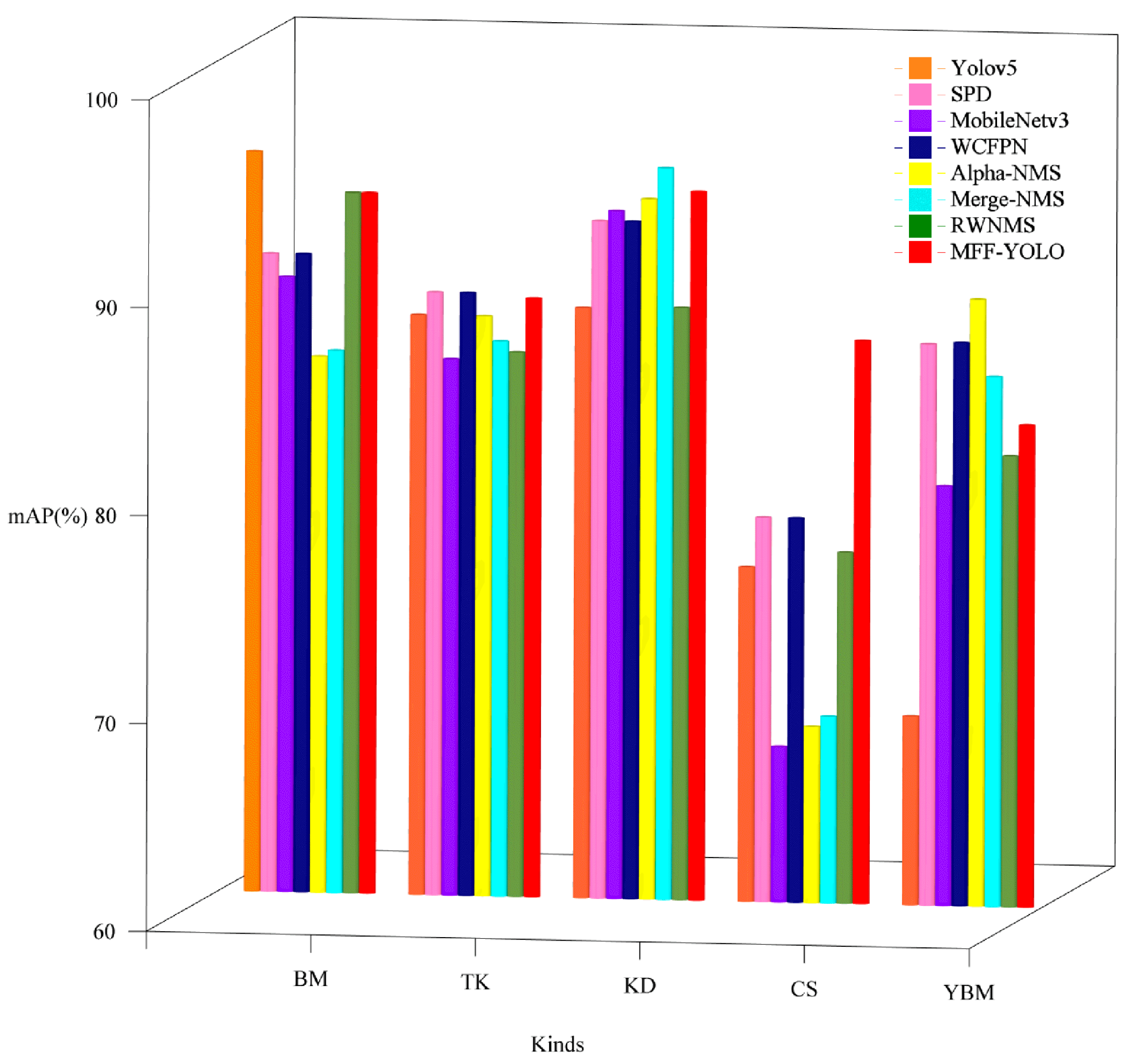
| Type | Average Accuracy Rate (%) | |||||
|---|---|---|---|---|---|---|
| Model | BM | TK | KD | CS | YBM | |
| Yolov5 | 95.6 | 87.9 | 88.4 | 76.1 | 69.1 | |
| SPD | 90.7 | 89.0 | 92.6 | 78.5 | 87.0 | |
| MobileNetv3 | 89.6 | 85.8 | 93.1 | 67.5 | 80.2 | |
| WCFPN | 90.7 | 89.0 | 92.6 | 78.5 | 87.1 | |
| Alpha-NMS | 85.8 | 87.9 | 93.7 | 68.5 | 89.2 | |
| Merge-NMS | 86.1 | 86.7 | 95.2 | 69.0 | 85.5 | |
| RWNMS | 93.7 | 86.2 | 88.5 | 76.9 | 81.7 | |
| MFF-YOLO | 93.7 | 88.8 | 94.1 | 87.1 | 83.2 | |
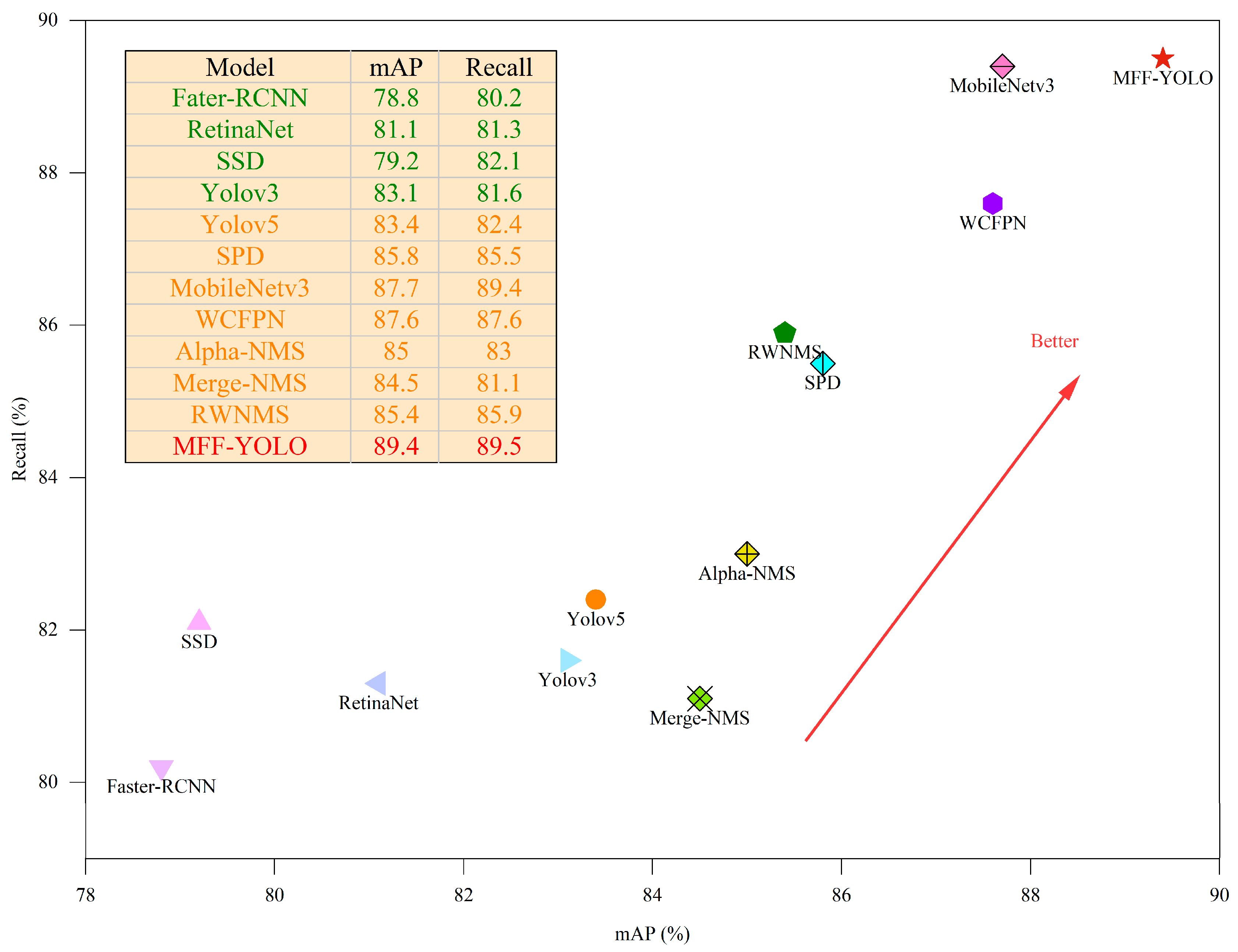
| Name | mAP@0.5 (%) | mAP@0.5:0.95 (%) | Precision (%) | Recall (%) | Gflops | FPS |
|---|---|---|---|---|---|---|
| Fater-RCNN | 78.8 | 48.8 | 78.6 | 80.2 | 88.2 | 18.2 |
| RetinaNet | 81.1 | 49.8 | 79.7 | 81.3 | 70.3 | 18.3 |
| SSD | 79.2 | 47.0 | 75.2 | 82.1 | 15.2 | 65.8 |
| Yolov3 | 83.1 | 49.1 | 80.3 | 81.6 | 154.6 | 16.4 |
| Yolov5 | 83.4 | 47.9 | 75.4 | 82.4 | 16.8 | 66.6 |
| SPD | 85.8 | 49.1 | 80.3 | 85.5 | 16.0 | 71.4 |
| MobileNetv3 | 87.7 | 50.4 | 81.0 | 89.4 | 15.3 | 50.0 |
| WCFPN | 87.6 | 51.6 | 82.2 | 87.6 | 33.1 | 52.6 |
| Alpha-NMS | 85.0 | 51.3 | 78.6 | 83.0 | 15.8 | 71.4 |
| Merge-NMS | 84.5 | 50.5 | 78.3 | 81.1 | 15.8 | 71.4 |
| RWNMS | 85.4 | 49.7 | 80.8 | 85.9 | 16.8 | 66.6 |
| MFF-YOLO | 89.4 | 50.8 | 82.2 | 89.5 | 33.3 | 50.0 |
Disclaimer/Publisher’s Note: The statements, opinions and data contained in all publications are solely those of the individual author(s) and contributor(s) and not of MDPI and/or the editor(s). MDPI and/or the editor(s) disclaim responsibility for any injury to people or property resulting from any ideas, methods, instructions or products referred to in the content. |
© 2023 by the authors. Licensee MDPI, Basel, Switzerland. This article is an open access article distributed under the terms and conditions of the Creative Commons Attribution (CC BY) license (https://creativecommons.org/licenses/by/4.0/).
Share and Cite
Zhu, A.; Wang, B.; Xie, J.; Ma, C. MFF-YOLO: An Accurate Model for Detecting Tunnel Defects Based on Multi-Scale Feature Fusion. Sensors 2023, 23, 6490. https://doi.org/10.3390/s23146490
Zhu A, Wang B, Xie J, Ma C. MFF-YOLO: An Accurate Model for Detecting Tunnel Defects Based on Multi-Scale Feature Fusion. Sensors. 2023; 23(14):6490. https://doi.org/10.3390/s23146490
Chicago/Turabian StyleZhu, Anfu, Bin Wang, Jiaxiao Xie, and Congxiao Ma. 2023. "MFF-YOLO: An Accurate Model for Detecting Tunnel Defects Based on Multi-Scale Feature Fusion" Sensors 23, no. 14: 6490. https://doi.org/10.3390/s23146490