DL development is a highly iterative and empirical process. It can be implemented in three steps, including choosing the initial weights and hyperparameter values, coding, and experimenting. These steps are interconnected through an interactive process.
4.1. CNN-Based Applications
CNN-based applications are attracting interest across a variety of domains, including optical sensor applications. In this section, some of the recent works that have been applying this model for optical sensors will be briefly presented
In [
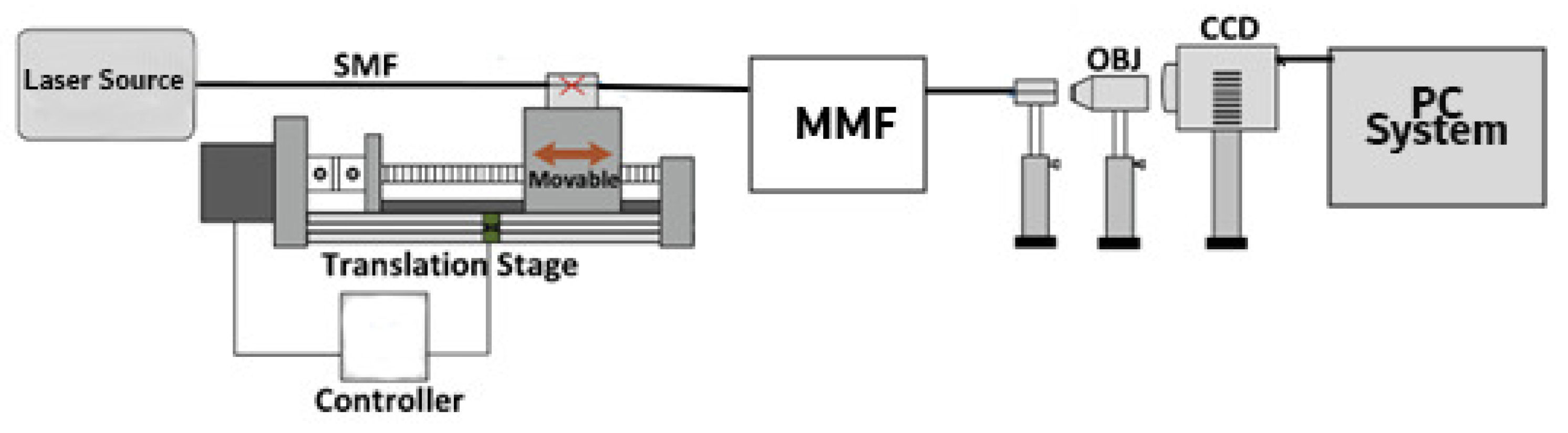
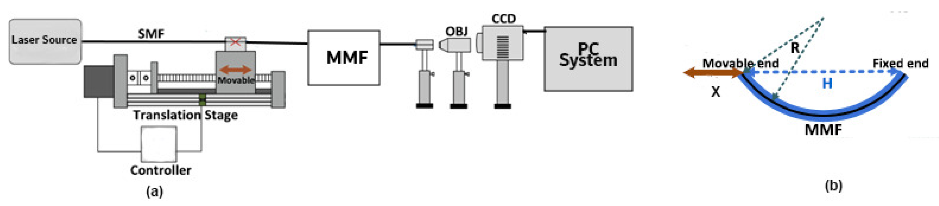
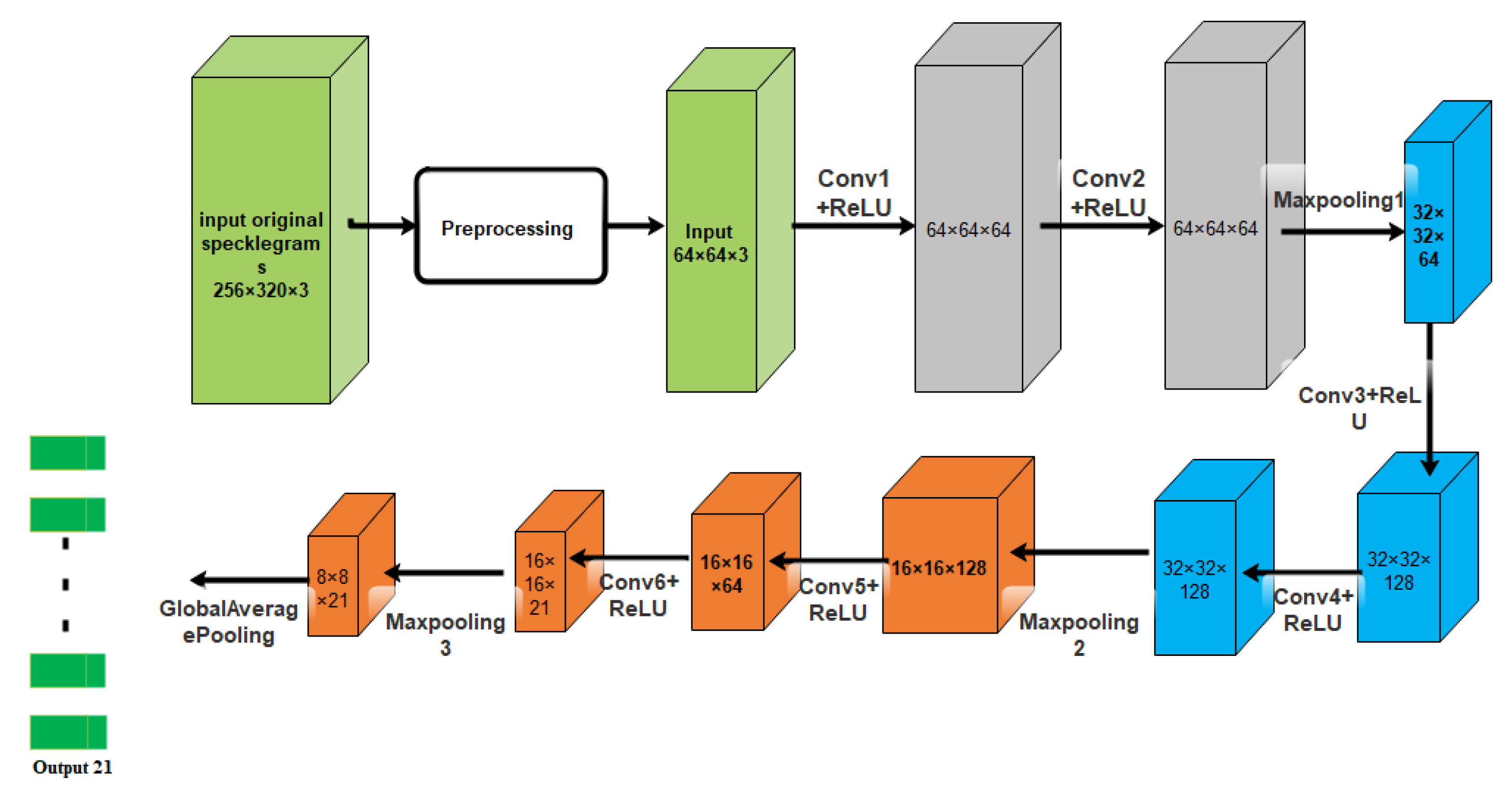
86], a CNN model was developed to comprehend an optical fibre curvature sensor. A large number of specklegrams have been automatically detected from the facet of multimode fibres (MMFs) in the experiments. The detected specklegrams were pre-processed and fed to the model for training, validation, and testing. The dataset was collected in the form of a light beam by designing an automated detecting experimental setup as shown in
Figure 6. The light beam was detected by a CCD camera with a resolution of
and a pixel size of 3.75 × 3.75
m
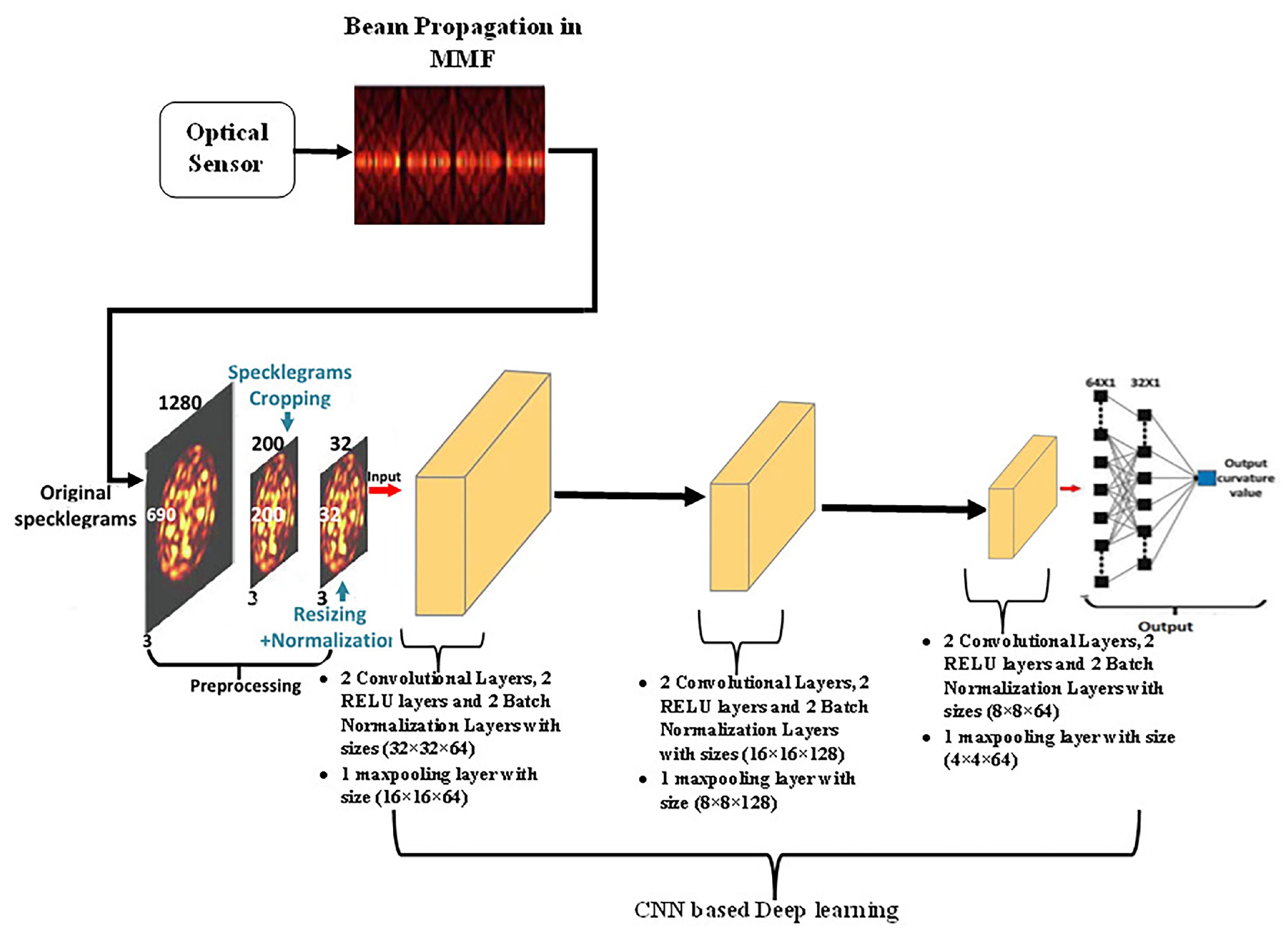
. As shown in
Figure 7, the architecture of VGG-Nets was adopted to build the CCN. The mean squared error (MSE) was then used as the loss function. The predicted accuracy of the proposed CNN was
of specklegrams with an error of curvature prediction within
m
. However, the learning-based scheme reported has the capability to only predict a solitary parameter and does not fully utilize the potential of DL.
In [
9], the authors proposed semi-supervised DL to detect a track. An experimental setup was created using a portion of a high-speed railway track and installing a distributed optical fibre acoustic system (DAS). In the proposed model, an image recognition model with a specific pre-processed dataset and an acquisitive algorithm for selecting hyperparameters was used.
The considered events supposed to be recognized in this model are shown in
Table 1.
In addition, the hyperparameters were selected based on an acquisitive algorithm. The obtained dataset after the augmentation process is shown in
Table 2.
Four structural hyperparameters were used in this work as shown in
Table 3. The obtained accuracy of the proposed model was 97.91%. However, it is important to highlight that the traditional methods have proven to execute improved spatial accuracy. Some other related works can be found in [
87,
88,
89,
90,
91,
92,
93,
94].
In [
95], a distributed optical fibre sensor using a hybrid Michelson–Sagnac interferometer was proposed. The motivation of the proposed model was to solve the complications of the incapability of the conventional hybrid structure to locate in the near and flawed frequency response. The proposed model utilized basic mathematical operations and a
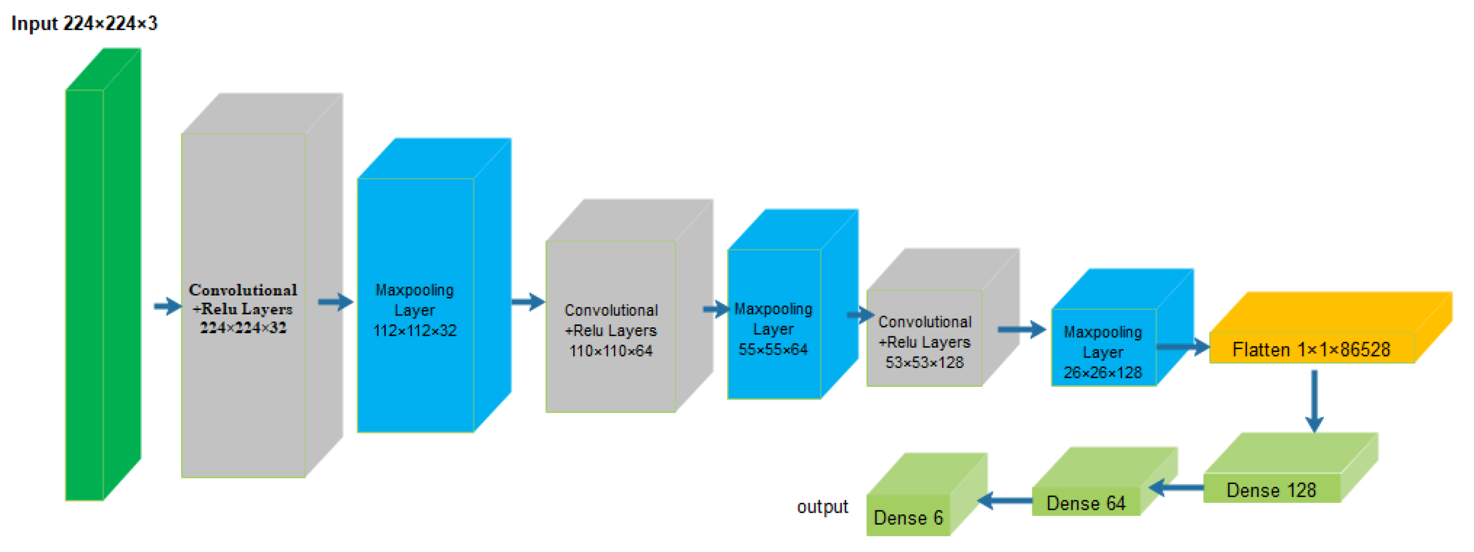
optical coupler to obtain two phase signals with a time difference that can be used for both location and pattern recognition. The received phase signals were converted into 2D images. These images were used as a dataset and fed into the CNN to obtain the required pattern recognition. The dataset contained 5488 images with six categories, and the size of each image was
in .jpg format. The description of the dataset is shown in
Table 4. The structural diagram of the used CNN is shown in
Figure 8. The accuracy of the proposed model was 97.83%. However, the sensing structure employed is relatively simple and does not consider factors such as the influence of backward scattered light.
In [
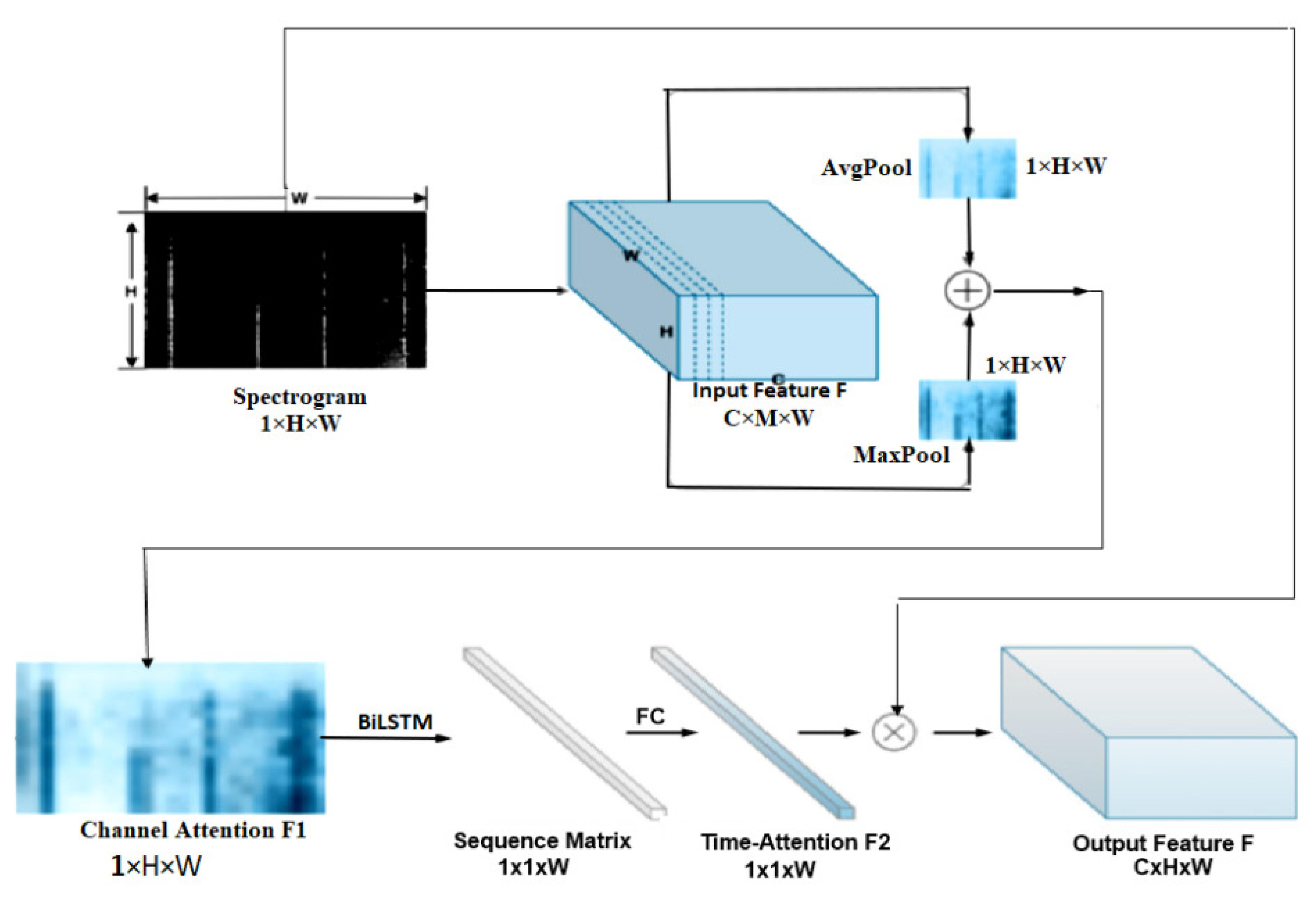
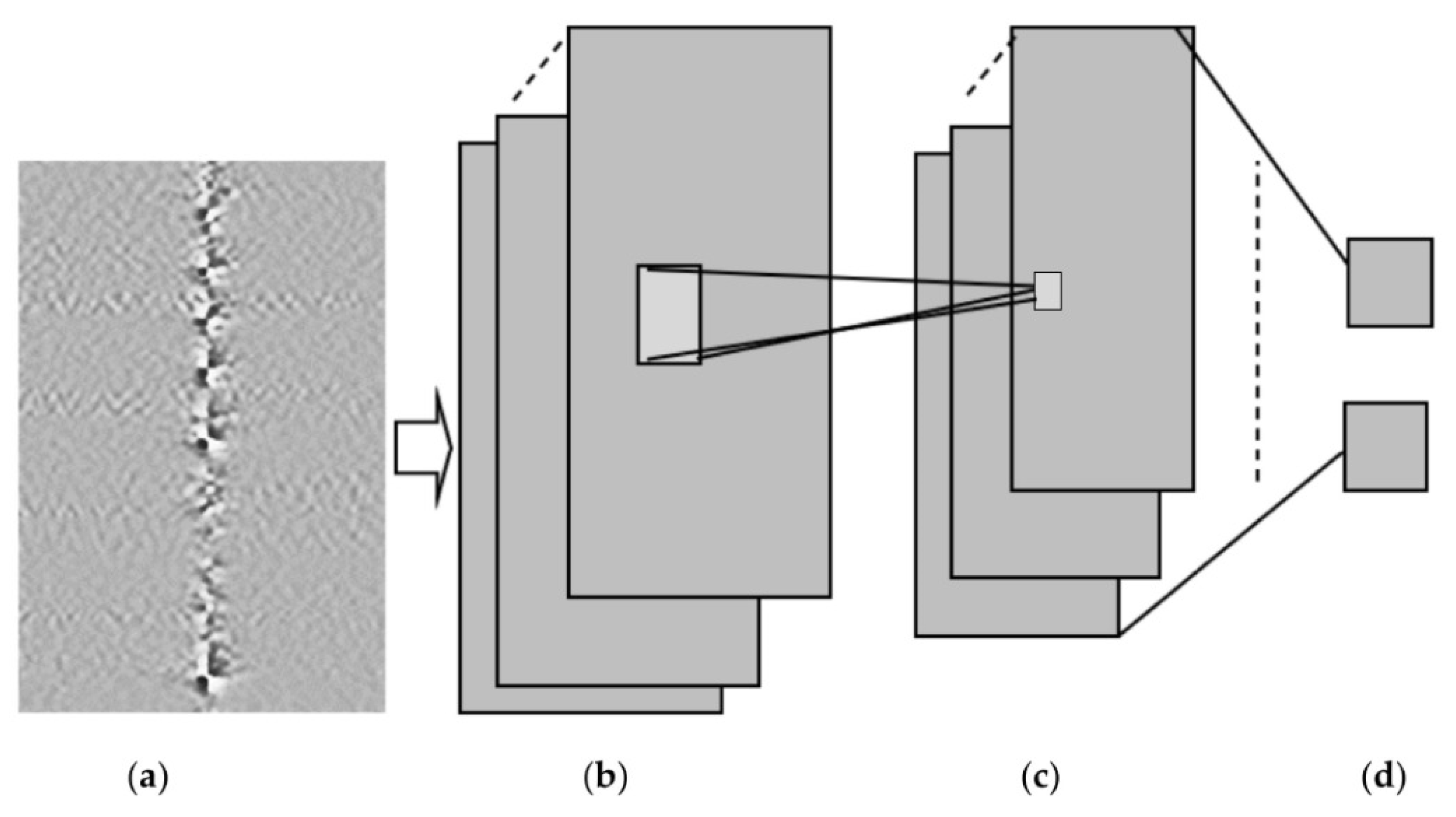
96], a DL model was proposed to extract time–frequency sequence correlation from signals and spectrograms to improve the robustness of the recognition system. The authors designed a targeted time attention model (TAM) to extract features in the time–frequency domain. The architecture of the TAM model comprises two stages, namely the convolution stage for extracting features and the time attention stage for reconstruction. The process of data streaming, domain transformation and features extraction to output is shown in
Figure 9. The knocking event is taken as an example. The convolution stage is used to extract characteristic features. Here, the convolutional filter established a local connection in the convolution and shared the weights between receiving domains. The pooling layers emphasized the shift-invariance feature. In addition, a usual CNN model was used as the backbone. As shown in
Figure 9, in the left stage, information was extracted from the spectrogram and transformed into a feature map
, where 1 represents the number of input channels (the grey image has one channel), while 128 and 200 represent the height and width of the input, respectively. The authors collected and labelled a large dataset of vibration scenes including
data points with eight vibration types. The experimental results indicated that this approach significantly improved the accuracy with minimal additional computational cost when compared to the related experiments [
97,
98]. The time attention stage was designed for the reconstruction of the features in which TAM was used to serve two purposes. The first purpose was to extract the sequence correlation by a cyclic element. The second purpose was to assign the weight matrices for the attention mechanism. F1 and F2 were unique in their emphasis on investigating the "where" and "what" features of time. An F-OTDR system was constructed to classify and recognize vibration signals. The F-OTDR system contained a sensing system and a producing system. This study was verified using a vibration dataset including eight different scenarios which were collected by an F-OTDR system. The achieved classification had an accuracy of 96.02%. However, this method did not only complicate the data processing procedure, but it also had the potential to result in the loss of information during the data processing phase.
In [
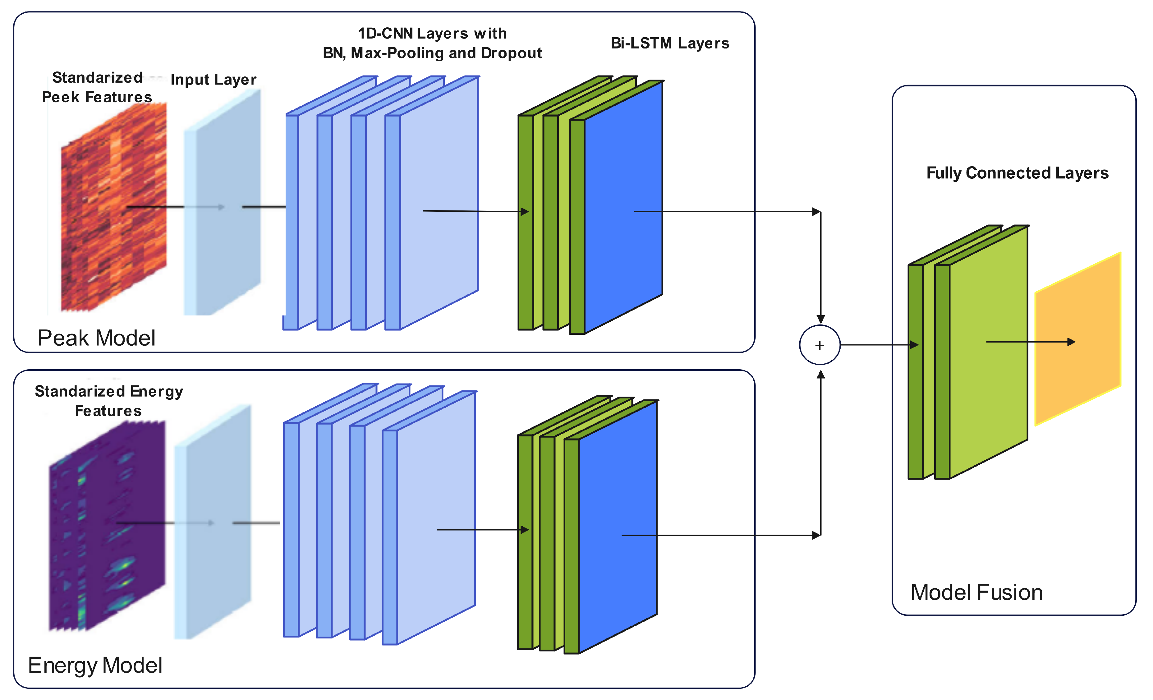
99], a real-time action recognition model was proposed for long-distance oil–gas PSEW systems using a scattered distributed optical fibre sensor. They used two methods to calculate two complementary features, a peak and an energy feature, which described the signals. Based on the calculated features, a deep learning network (DLN) was built for a new action recognition. This DLN could effectively describe the situation of long-distance oil–gas PSEW systems. The collected datasets were 494 GB with several types of noise at the China National Petroleum Corporation pipeline. The collected signal involved four types of events containing background noise, mechanical excavation, manual excavation, and vehicle driving. As shown in
Figure 10, the architecture of the proposed model consisted of two parts. The first part dealt with the peak, while the second part dealt with the energy. Each part consisted of many layers, including ConvD1, batch normalization, maxpool, dropout, Bi-LSTM, and a fully connected layer. Any damage event could be allocated and identified with accuracies of 99.26 and 97.20% at 500 and 100 Hz, respectively. Nonetheless, all the aforementioned methods consider an acquisition sample as a singular vibration event. However, for dynamic time-series identification tasks, the ratio of valid data within a sample relevant to the overall data was not constant. This means that the position of the label in relation to the valid portion of the input sequence remained uncertain. Further related research can be reviewed in [
100,
101,
102].
In [
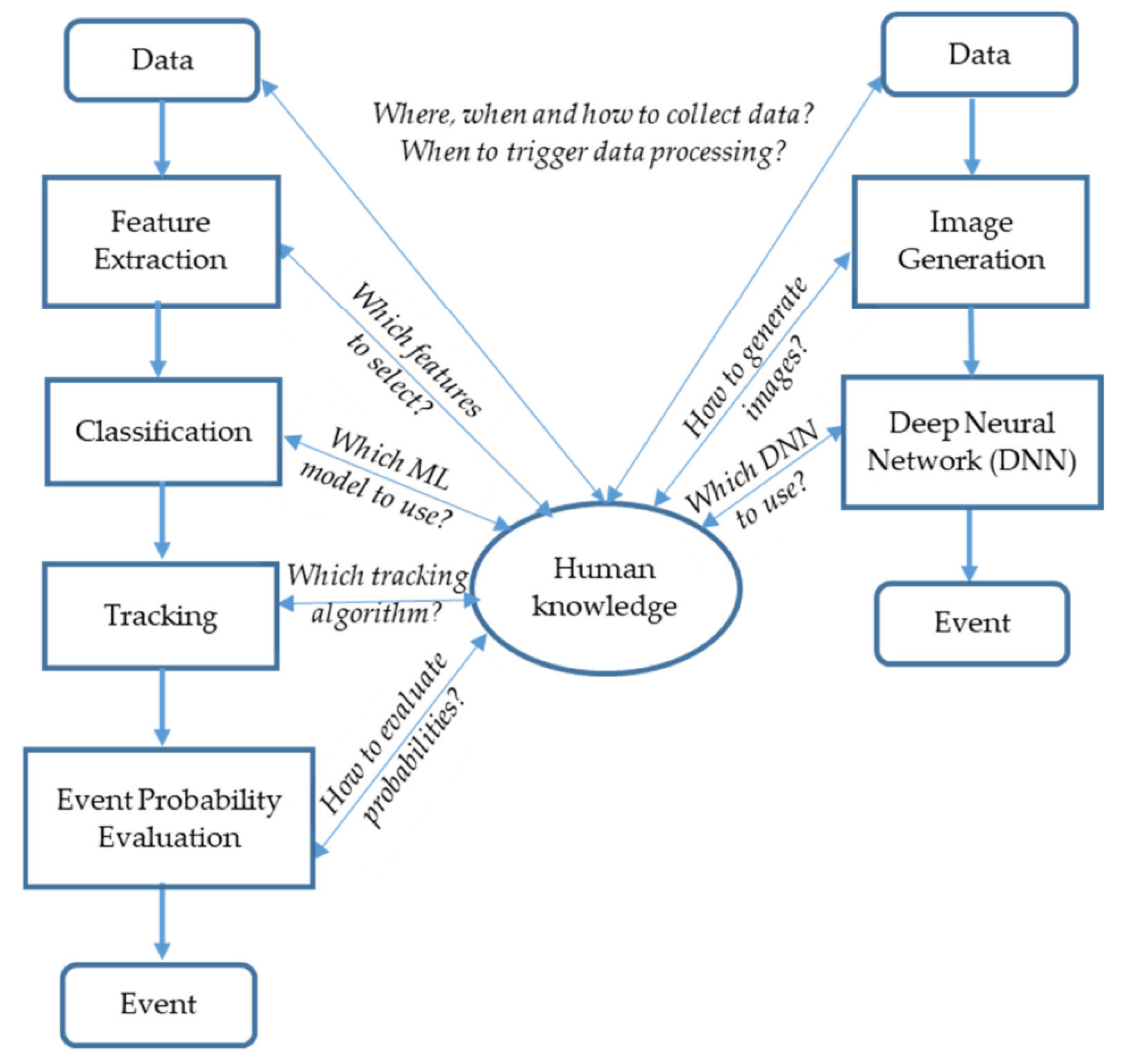
103], the authors presented the application of signal processing and ML algorithms to detect events using signals generated based on DAS along a pipeline. ML and DL approaches were implemented and combined for event detection as shown in
Figure 11. A novel method to efficiently generate training dataset was developed. Excavator and none-excavator events were considered.
The sensor signals were converted into a grey image to recognize the events depending on the proposed DL model. The proposed model was evaluated in real-time deployment within three months in a suburban location as shown in
Figure 12.
The results showed that DL is the most promising approach due to its advantages over ML as shown in
Table 5. However, the proposed model only differentiated between two events, namely ‘excavator’ and ‘non-excavator’, while there are multiple distinct events. Additionally, the system was evaluated in a real-time arrangement for a duration of three months in a suburban area. Yet, for further validation and verification, it is crucial to conduct tests in different areas and over an extended period of time.
In [
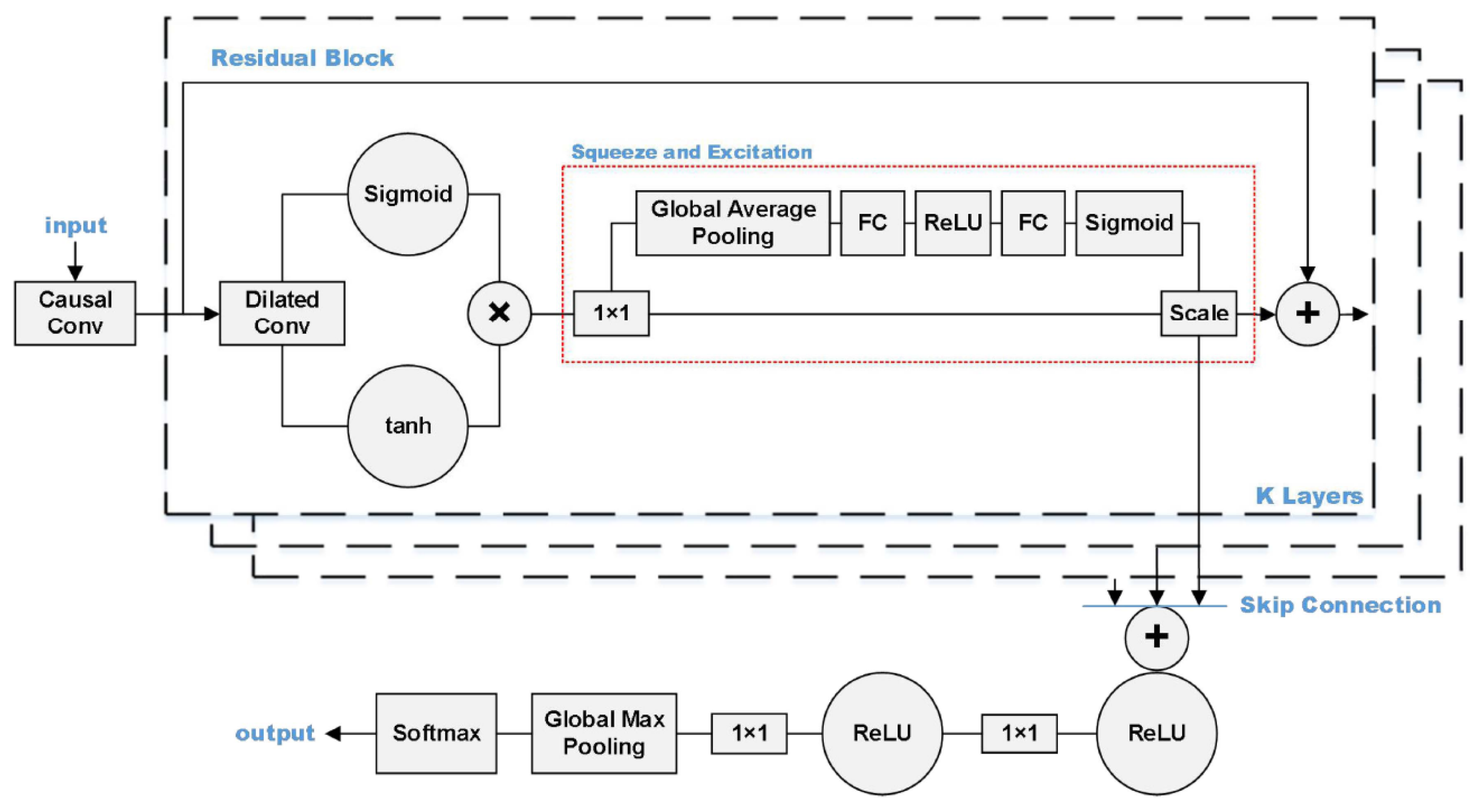
104], an improved WaveNet was applied to recognize manufactured threatening events using distributed optical fibre vibration sensing (DVS). The improved WaveNet is called SE-WaveNet (squeeze and excitation WaveNet). WaveNet is a 1D CNN (1D-CNN) model. As a deep 1D-CNN, it can quickly achieve training and testing while also boasts a large receptive field that enables it to retain complete information from 1D time-series data. The structure of the SE functions in synchronization with the residual block of WaveNet in order to recognize 2D signals. The SE structure functions using an attention mechanism, which allows the model to focus on channel features to obtain more information. It can also suppress insignificant channel features. The structure of the proposed model is shown in
Figure 13. The input of the SE-WaveNet is an n × m matrix, synthesized from the n-points of spatial signals and the m-groups of time signals. The used dataset is shown in
Table 6. The results showed that the SE-WaveNet accuracy can reach approximately 97.73%. However, it is important to note that the model employed in this study was only assessed based on a limited number of events, and further testing is necessary to evaluate its performance in more complex events, particularly in engineering-relevant applications. Additionally, further research is needed to validate the effectiveness of the SE-WaveNet in practical, real-world settings.
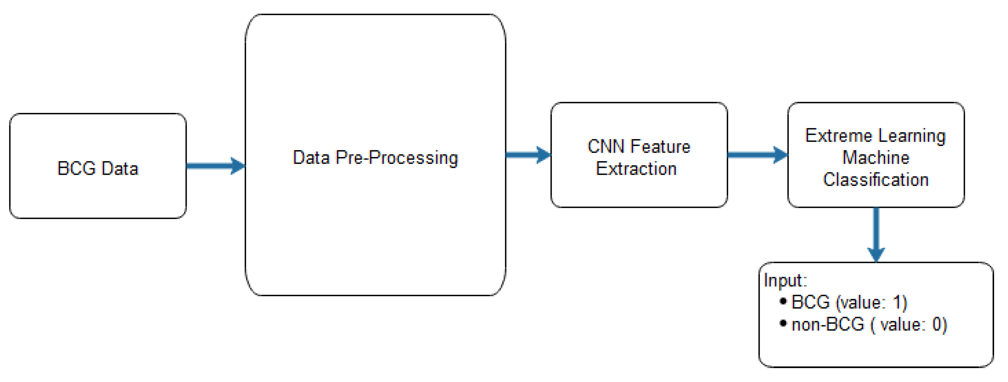
In [
14], a CNN and an extreme learning machine (ELM) were applied to discriminate between ballistocardiogram (BCG) and non-BCG signals. CNNs were used to extract relevant features. As for ELM, it is a feedforward neural network that takes the features extracted from CNN as the input and provides the category matrix as an output [
105]. The architecture of the proposed CNN-ELM and the proposed CNN are shown in
Figure 14 and
Table 7, respectively.
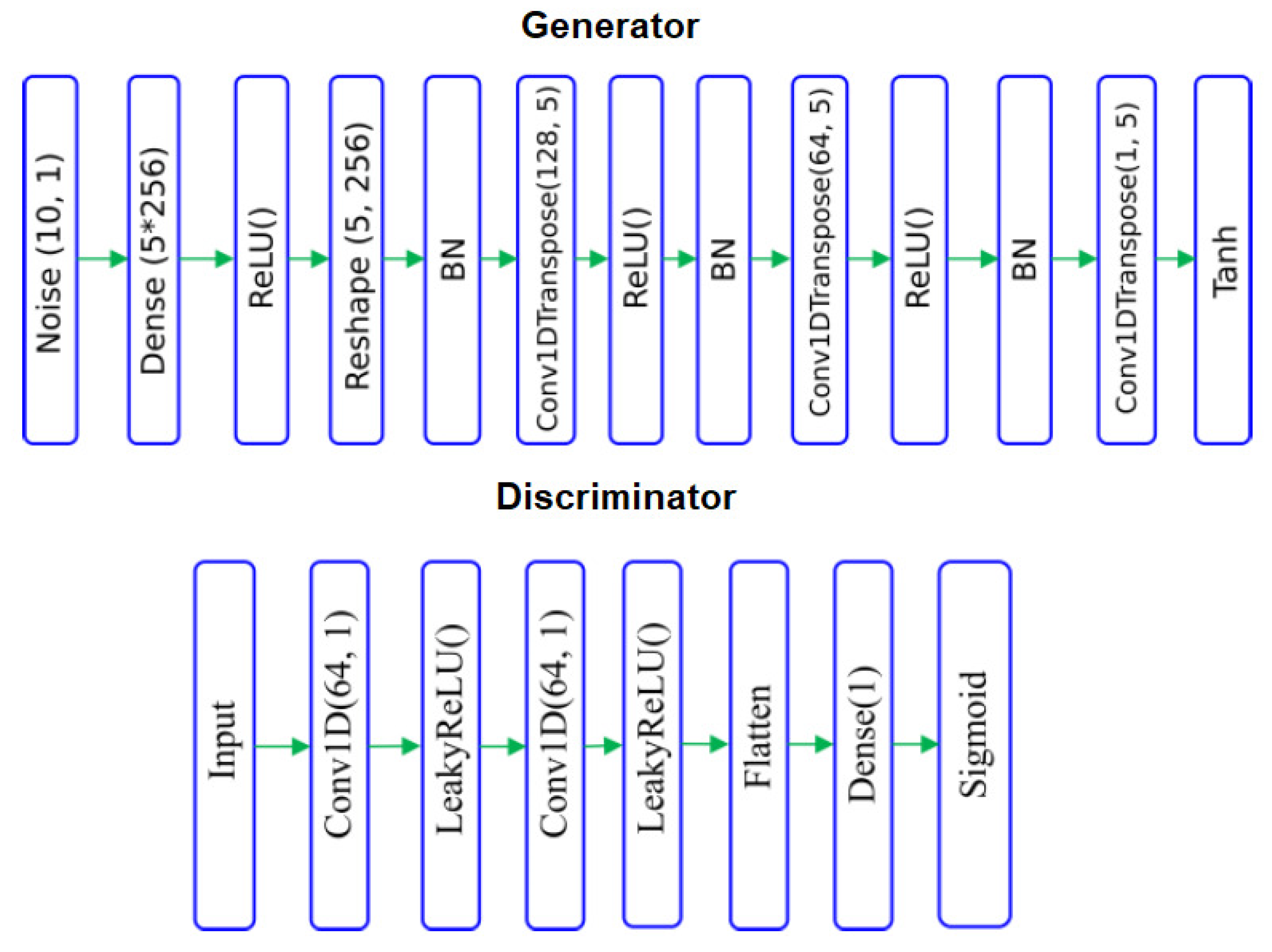
BCG signals were obtained with a micro-bend fibre optical sensor based on IoT, taken from ten patients diagnosed with obstructive sleep apnoea and submitted for drug-induced sleep endoscopy. To balance the BCG (ballistocardiogram) and non-BCG signal samples, three techniques were employed: undersampling, oversampling, and generative adversarial networks (GANs). The performance of the system was evaluated using ten-fold cross-validation. Using GANs to balance the data, the CNN-ELM approach yielded the best results with an average accuracy of 94%, a precision of 90%, a recall of 98%, and an F-score of 94%, as shown in
Table 8. Inspired by [
106], the architecture of the used model is presented in
Figure 15, showing balanced BCG and non-BCG chunks. Other relevant works were presented in [
107,
108].
In [
11], the efficiency and accuracy enhancements of the bridge structure damage detection were addressed by monitoring the deflection of the bridge using a fibre optic gyroscope. A DL algorithm was then applied to detect any structural damage. A supervised learning model using CNN to perform structural damage detection was proposed. It contained eleven hidden layers constructed to automatically identify and classify bridge damage. Furthermore, the Adam optimization method was considered and the used hyperparameters are listed in
Table 9. The obtained accuracy of the proposed model was 96.9% which was better than the random forest (RF), which was 81.6%, the SVM which was 79.9%, the k-nearest neighbor (KNN) which was 77.7%, and the decision trees (DT). Following the same path, comparable work was performed in [
109,
110].
The authors in [
111] proposed an intrusion pattern recognition model based on a combination of Gramian angular field (GAF) and CNN, which possessed both high speed and accuracy rate in recognition. They used the GAF algorithm for mapping 1D vibration-sensing signals into 2D images with more distinguishing features. The GAF algorithm retained and highlighted the distinguishing differences of the intrusion signals. This was beneficial for CNN to detect intrusion events with more subtle characteristic variation differences. A CNN-based framework was used for processing vibration-sensing signals as input images. According to the experimental results, the average accuracy rate for recognizing the three natural intrusion events, light rain, wind blowing, and heavy rain, and the three human intrusion events, impacting, knocking, and slapping, on the fence was found to be 97.67%. With a response time of 0.58 seconds, the system satisfied the real-time monitoring requirements. By considering both accuracy and speed, this model achieved automated recognition of intrusion events. However, the application of complex pre-processing and denoising techniques to the original signal presented a challenge for intrusion recognition systems when it came to effectively addressing emergency response scenarios. Relevant work following a similar pattern was presented in [
112].
A bending recognition model using the analysis of MMF specklegrams with diameters of 105 and 200 µm was proposed and assessed in [
113]. The proposed model utilized a DL-based image recognition algorithm. The specklegrams detected from the facet of the MMF were subjected to various bendings and then utilized as input data.
Figure 16 shows the used experimental setup to collect and detect fibre specklegrams.
The architecture of the model was based on VGG-Nets as shown in
Figure 17.
The obtained accuracy of the proposed model for two multimode fibres is shown in
Table 10.
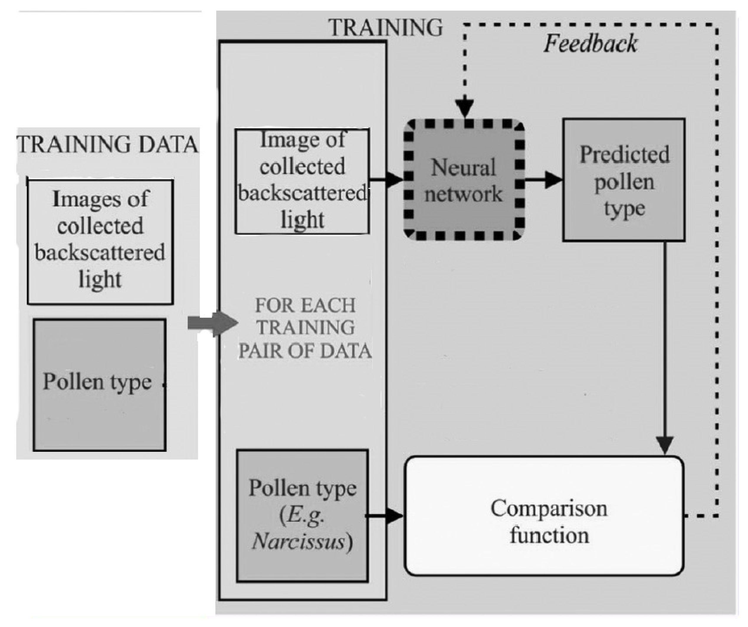
The authors in [
122] used a CNN to demonstrate the capability for the identification of specific species of pollen from backscattered light. Thirty-core optical fibre was used to collect the backscattered light. The input data provided to the CNN was from camera images which were further divided into two sets, distance prediction and particle identification. In the first type, the total number of collected images was 1500, by which 90% of them were used as a training set and 10% were used as a validation set of the CNN. In the second type, 2200 images were collected and 90% of them were used as a training set and 10% were used as a validation set. The training procedure of the proposed model is depicted in
Figure 18. The second version of ResNet-18 ([
123,
124]) was used to propose the required model with batch normalization [
125] with a mini-batch size of 32 and a momentum of 0.95. The output was a single regression (single output). The neural network, trained to identify pollen grain types, achieved a real-time detection accuracy of approximately 97%. The developed system can be used in environments where transmission imaging is not possible or suitable.
In [
13], a DL-based distributed optical fibre-sensing system was proposed for event recognition. A spatio-temporal data matrix from an F-OTDR system was used as the input data served to the CNN. The proposed method had advantageous characteristics, such as grey-scale image transformation and bandpass filtering, which were needed for pre-processing and classification instead of the usual complex data processing, small size, and high training speed, and excessive requirements for classification accuracy. The developed system was applied to recognize five distinct events involving background, jumping, walking, digging with a shovel, and striking with a shovel. The collected data were split into two types as shown in
Table 11. The combined dataset for the five events consisted of 5644 instances.
Some common CNNs were examined, and the results are shown in
Table 12.
The considered training parameters for all CNNs were the same. The total training steps were 50,000, the learning rate was 0.01, and the adopted optimizer was the root mean square prop (RMSProp) [
126]. This work concluded that the VGGNet and GoogLeNet obtained better classification accuracy (greater than 95%) and GoogLeNet was selected to be the basic CNN structure due its model size. For further improvement of the model, Inception-v3 of GoogLeNet was used.
Table 13 shows the classification accuracy achieved for the five events. The authors also optimized the network by tuning the size of some layers of the model.
Table 14 shows the comparison between the optimized model and Inception-v3. However, it is important to note that this study trained the network using relatively small datasets consisting of only 4000 samples. Moreover, traditional data augmentation strategies employed in image processing, such as image rotation, cannot be directly applied to feature maps generated from fibre optic-sensing data.
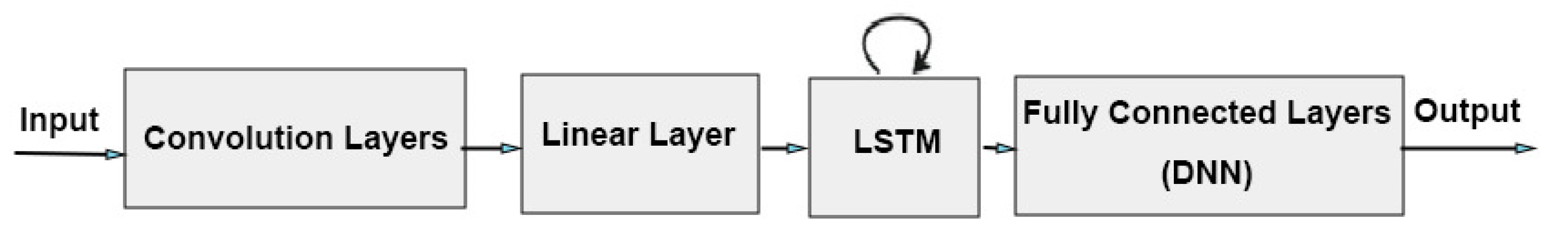
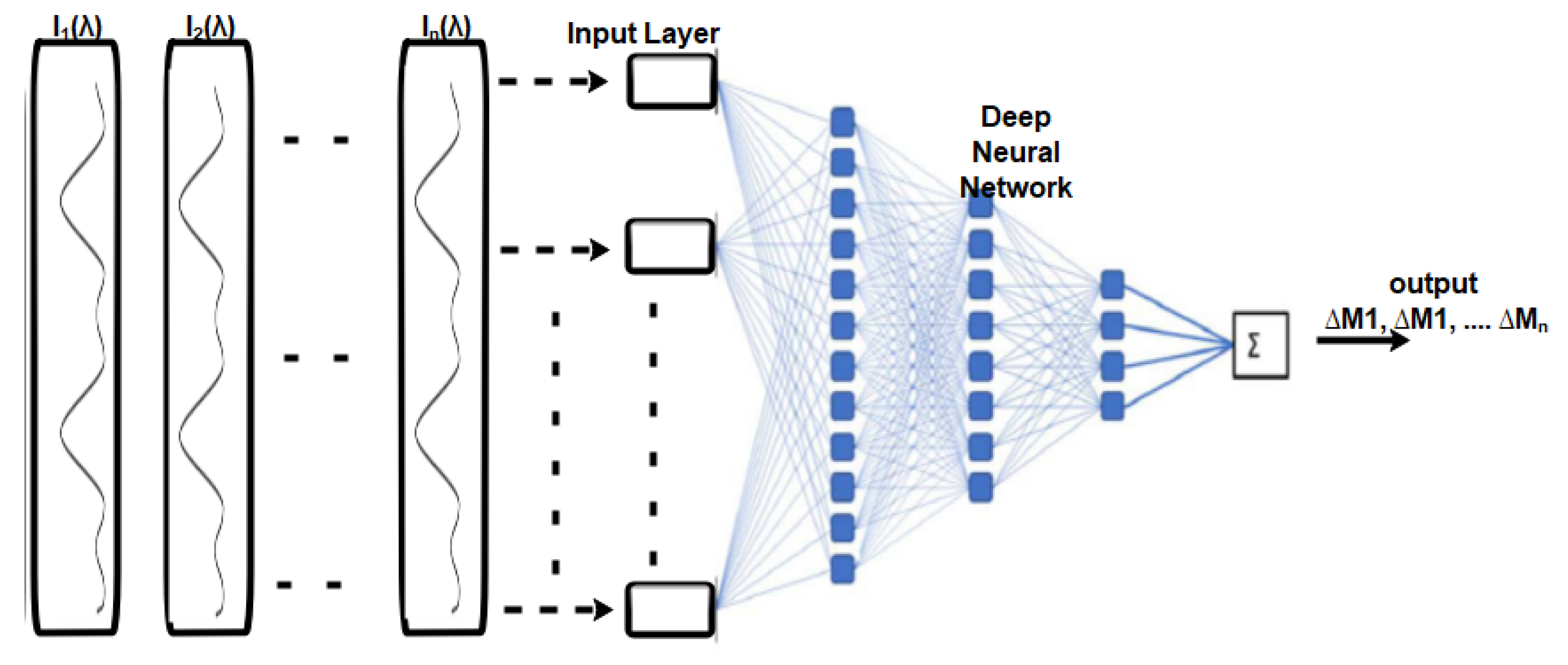
In [
8], the authors designed a DNN to identify and classify external intrusion signals from a 33 km optical fibre-sensing system in a real environment. In that article, the time-domain data was located directly into a DL model to deeply learn the characteristics of the destructive intrusion events and establish a reference model. This model included two CNN layers, one linear layer, one LSTM layer, and one fully connected layer as shown in
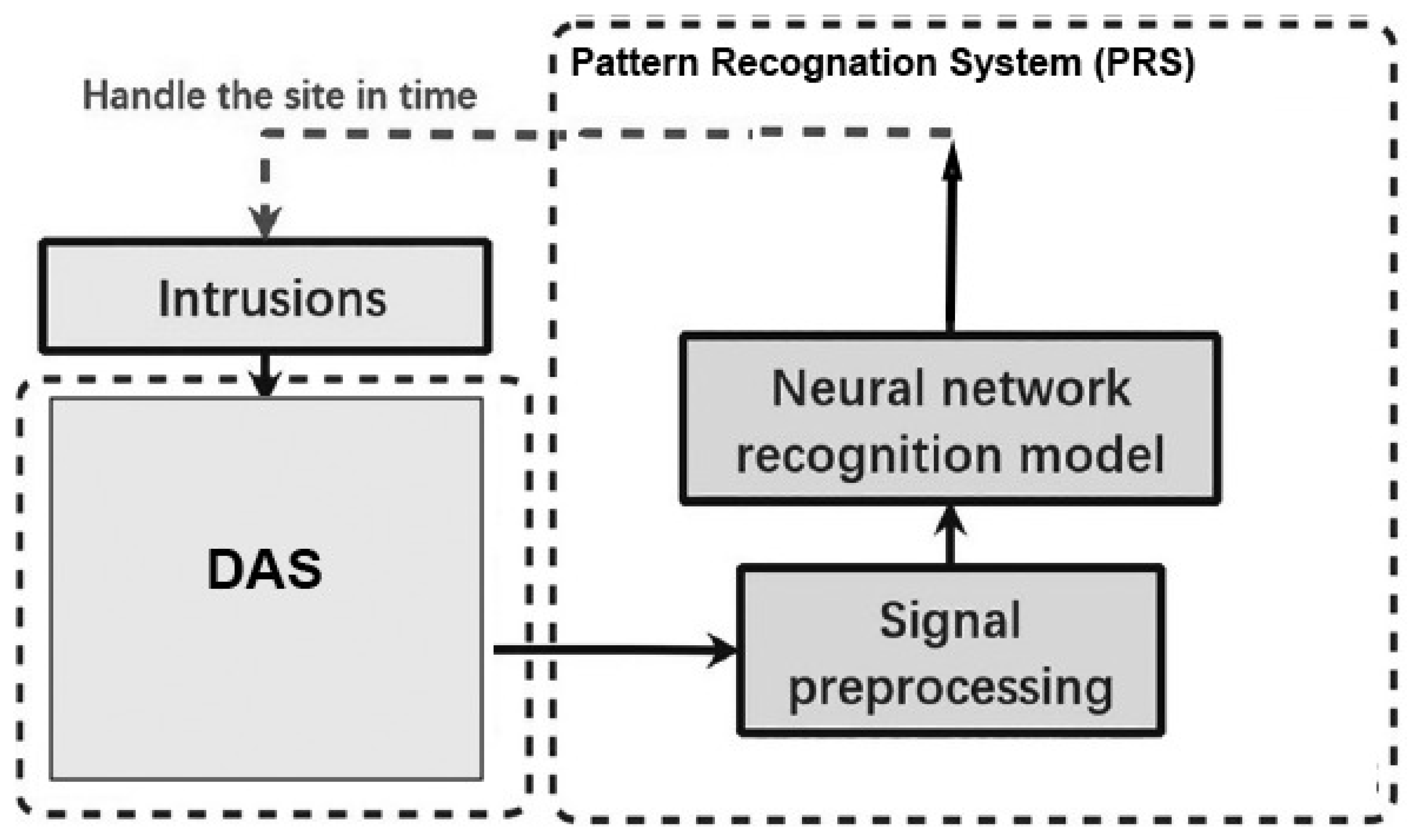
Figure 19. It was called the convolutional, long short-term memory, fully connected deep neural network (CLDNN). The model effectively learned the signal characteristics captured by the DAS and was able to process the time-domain signal directly from the distributed optical fibre vibration-monitoring systems. It was found to be simpler and more effective than feature vector extraction through the frequency domain. The experimental results demonstrated an average intrusion event recognition rate exceeding 97% for the proposed model.
Figure 20 shows the DAS system using the F-OTDR and the pattern recognition process using the CLDNN. However, the proposed model was not evaluated as a prospective solution for addressing the issue of sample contamination caused by external environmental factors, which can lead to a decline in the recognition accuracy. Other related work can be viewed in [
127].
A novel method was developed in [
12] to efficiently generate a training dataset using GAN [
128]. End-to-end neural networks were used to process data collected using the DAS system. The proposed model’s architecture utilized the VGG16 network [
23]. The purpose of the proposed model was to detect and localize seismic events. One extra convolutional layer was added to match the image size then a fully connected layer was added at the end of the model. Batch normalization for regularization and an ReLU activation function were used. The model was tested with experimentally collected data with a 5 km long DAS sensor, and the obtained classification accuracy was 94%. Nevertheless, achieving a reliable automatic classification using the DAS system remains computationally and resource-intensive, primarily due to the demanding task of constructing a comprehensive training database, which involves collecting labelled signals for different phenomena. Furthermore, overly complex approaches may render real-time applications impractical, introducing potential processing-delay issues. Other works in the same direction have been presented in [
129,
130].
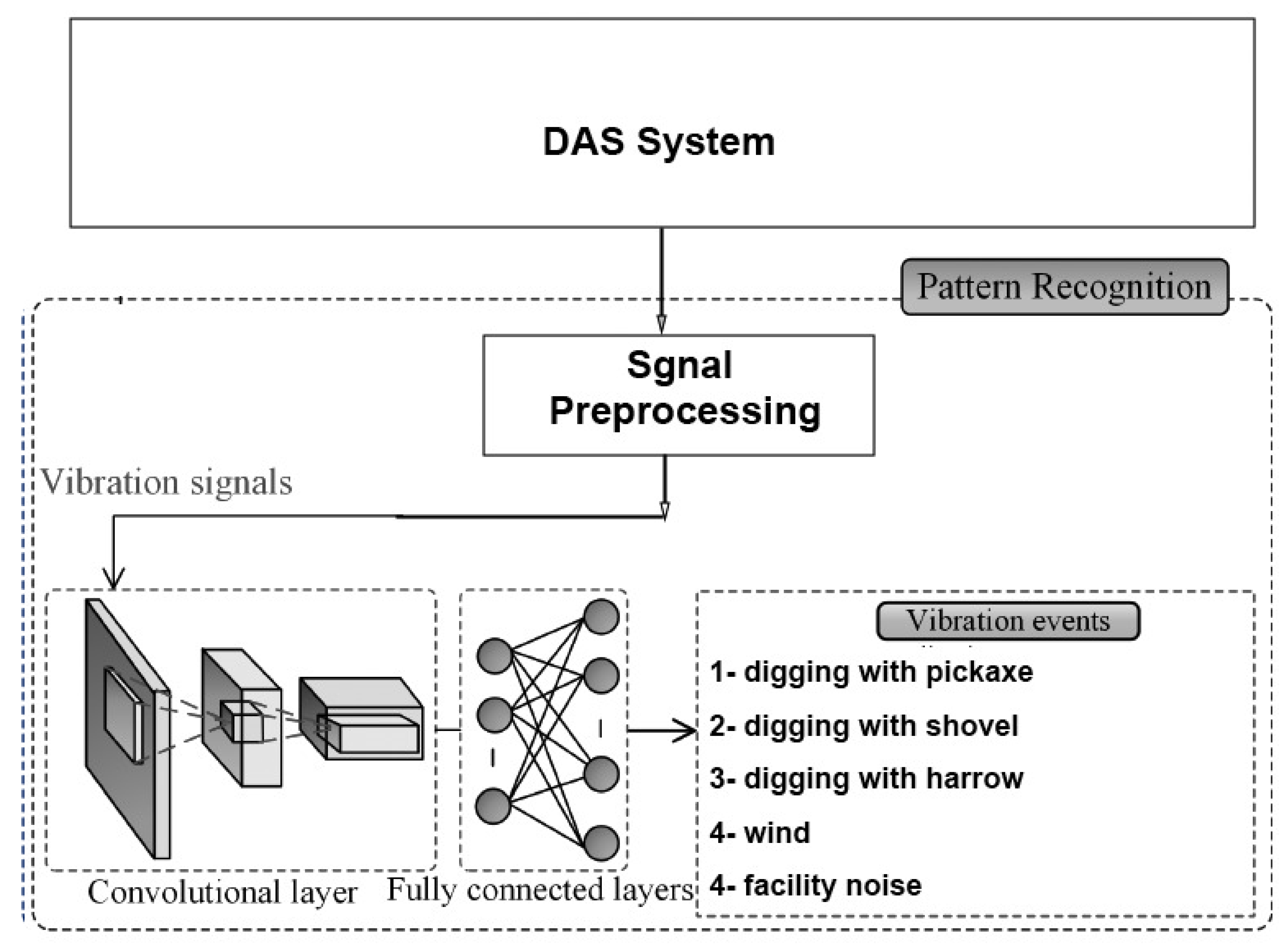
In [
127], the authors presented a DL model to recognize six activities, including walking, digging with a shovel, digging with a harrow, digging with a pickaxe, facility noise, and strong wind. The DAS system based on F-OTDR was presented along with novel threat detection, signal conditioning, and threat classification techniques. The CNN architecture used for the classification was trained with real sensor data and consisted of five layers, as illustrated in
Figure 21. In this algorithm, an RGB image with dimensions 257 × 125 × 3 was constructed. This image was constructed for each detection point on the optical fibre, helping determine the classification of the event through the network. The results indicated that the accuracy of the threat classification exceeded 93%. However, increasing the depth of the network structure in the proposed model will unavoidably results in a significant slowdown in the training speed and potentially lead to overfitting.
In the study published in [
131], the authors proposed an approach to detect defects in large-scale PCBs and measure their copper thickness before the mass production process using a hybrid optical sensor HOS based on CNN. The method involved combining microscopic fringe projection profilometry (MFPP) with lateral shearing digital holographic microscopy (LSDHM) for imaging and defect detection by utilizing an optical microscopic sensor containing minimal components. This allowed for more precise and accurate identification of diverse types of defects on the PCBs. The proposed approach had the potential to significantly improve the quality control process in PCB manufacturing, leading to more efficient and effective production. The researchers’ findings demonstrate a remarkable success rate with an accuracy of 99%.


