
Robust Vector BOTDA Signal Processing with Probabilistic Machine Learning
 , , , and
Abstract
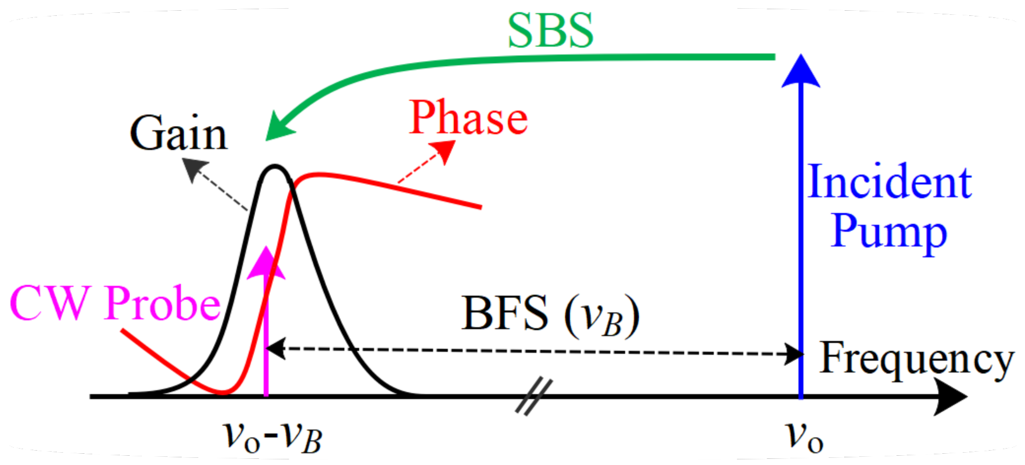
:1. Introduction
2. Mathematical Background
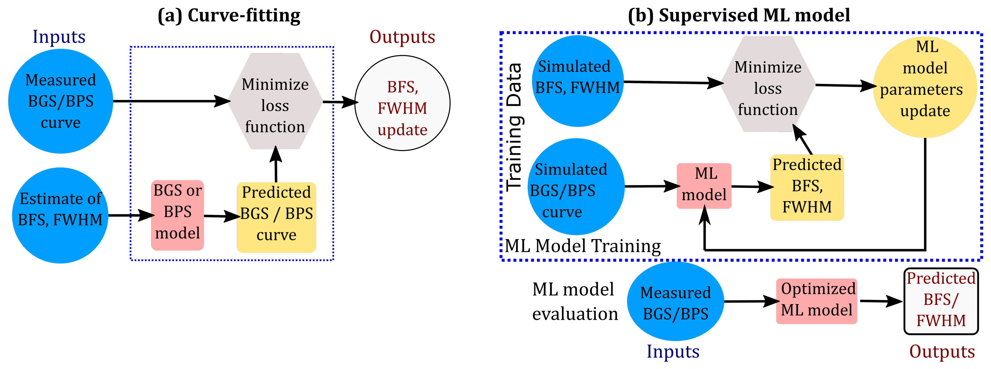
2.1. Curve Fitting Approach
2.2. Machine Learning Approach
2.3. Comparison of Curve Fitting vs. Machine Learning for BFS Extraction
- Data Processing Time: The computational advantage of the ML approach over the CF approach is evident when comparing the schematics of both approaches, as shown in Figure 2. The CF approach requires repeating the optimization iterations for each BGS, while the ML approach can predict the BFS and FWHM directly from the BGS measurements using Equation (7), once the ML model is trained offline.
- Interpretability: However, the CF approach is more interpretable since the function can be chosen based on the underlying optical physics knowledge. On the other hand, no such reasoning exists to construct in the ML approach and several different ML models have been proposed in the literature.
- Robustness: A key feature of a robust signal processing algorithm is its ability to accurately quantify the confidence/uncertainty in predictions. As mentioned earlier, curve fitting approaches use regression to estimate parameters and can yield CIs of the parameter estimates. However, the ML approach (Equation (5)) can not be used directly to estimate the CIs since the term does not represent the sensor measurement error. Instead, in Equation (5) should be interpreted as prediction error with an unknown probability distribution due to the nonlinear nature of . Subsequently, the ML approach provides BFS estimates without providing a measure of uncertainty/confidence (i.e., confidence intervals or error bars) of the BFS predictions. With the increasing adoption of deep neural networks for BOTDA processing, it is even more crucial that the BFS be estimated along with its confidence level, in order to avoid over-fitting.
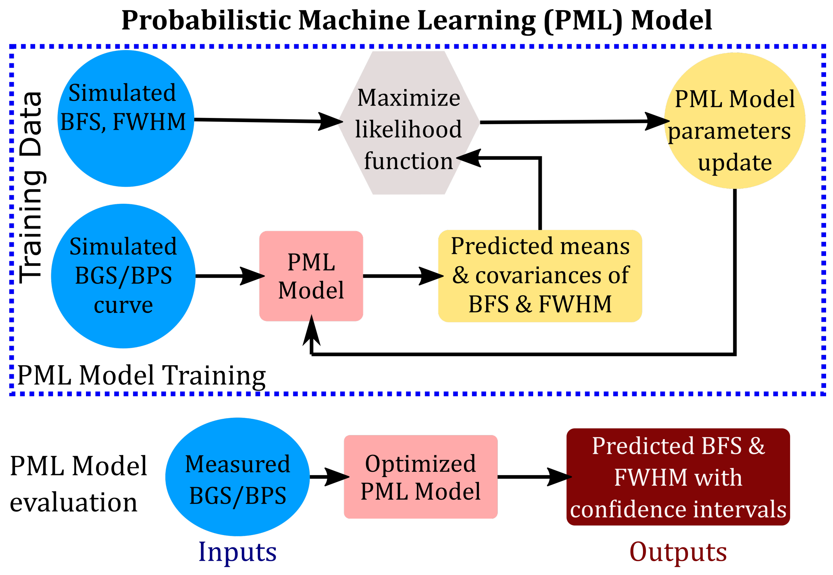
3. Proposed Probabilistic Machine-Learning-Based BFS Extraction
- Mean vector directly predicts the means of BFS () and FWHM (w) from BGS/BPS measurements using a suitable ML model
- Standard deviation matrix quantifies the uncertainty in estimates of BFS () and FWHM (w) due to the noise in underlying measurements
- Robustness: The PML approach prevents overfitting that arises when using ML and DNN models to represent .
- Speed: It inherits the computational advantages of the ML approach and enables fast processing of BOTDA data with simultaneous assessment of prediction uncertainties.
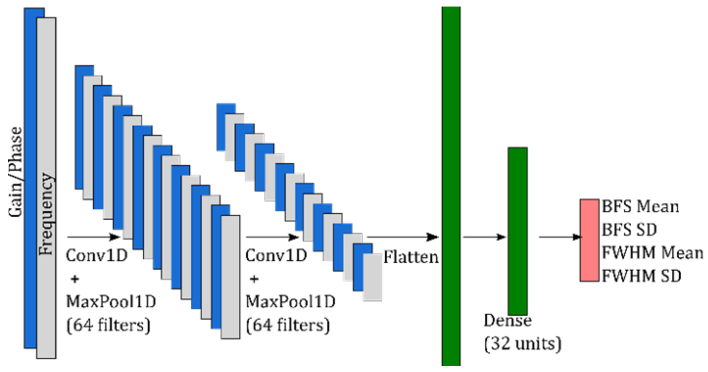
4. PML Model Development and Training
4.1. PML Model Training
- Uniformly sample s, , and w from the bounds in Equation (19) to obtain
- Simulate gain and phase values for each of the n frequencies and for using a suitable spectrum model.This work has chosen Lorentzian BGS and BPS [7] (Equations (22) and (23)) given by the following:where is the Brillouin gain amplitude, w is the Brillouin linewidth or FWHM, and is the BFS.
- Sample and add Gaussian noise corresponding to the noise amplitude to obtain training dataset sample
4.2. PML Model Architecture
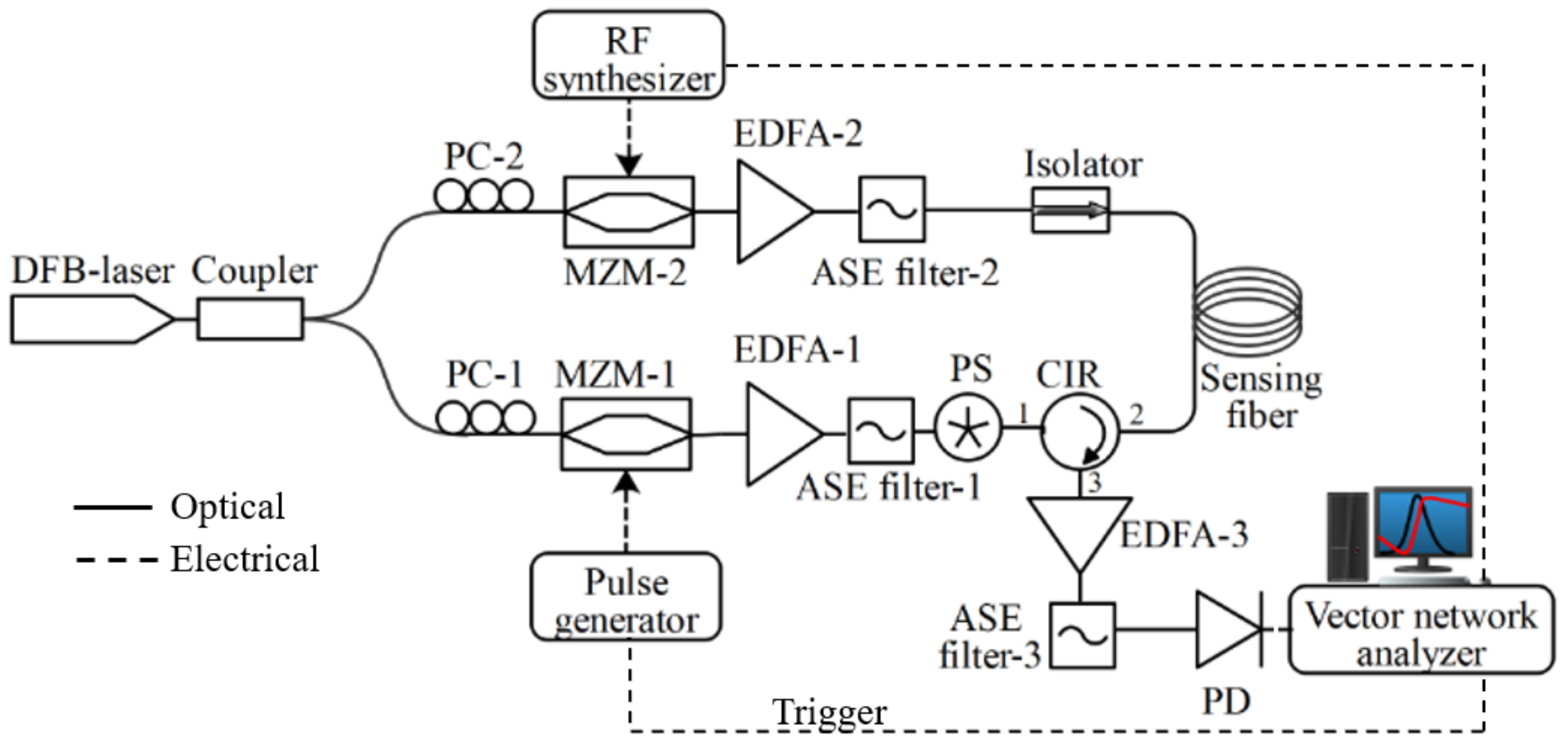
5. Experimental Setup
6. Results and Discussions
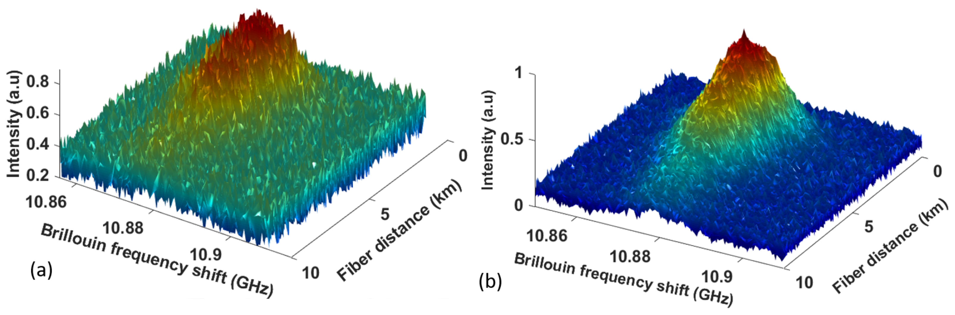
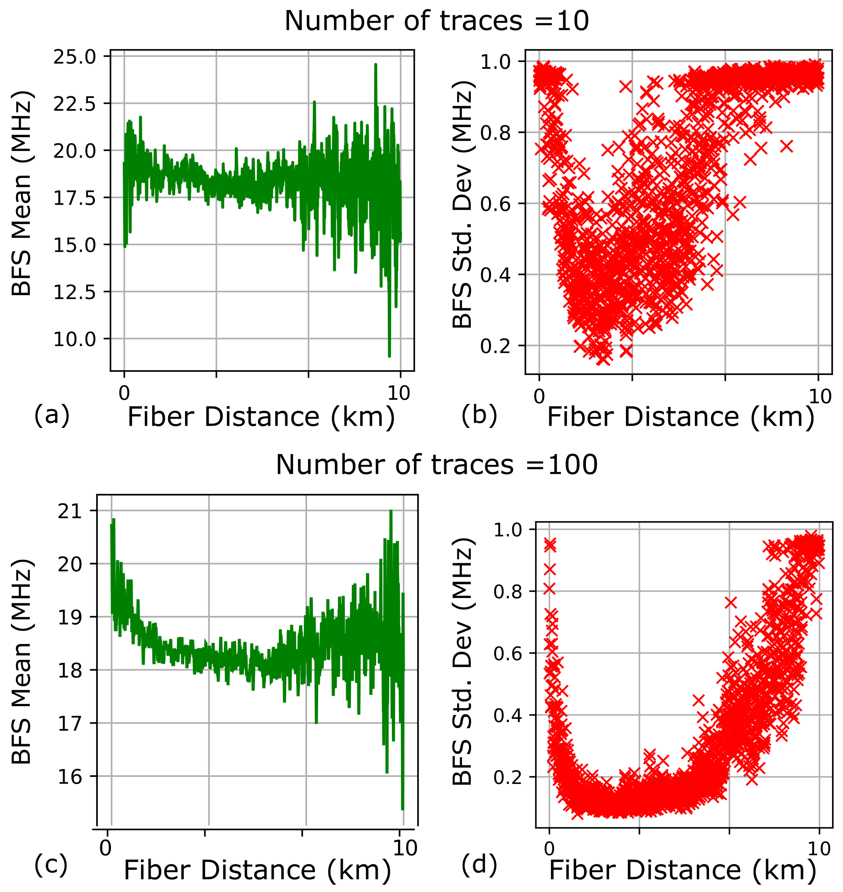
6.1. Custom BOTDA System Using 10 km Long Sensing Fiber
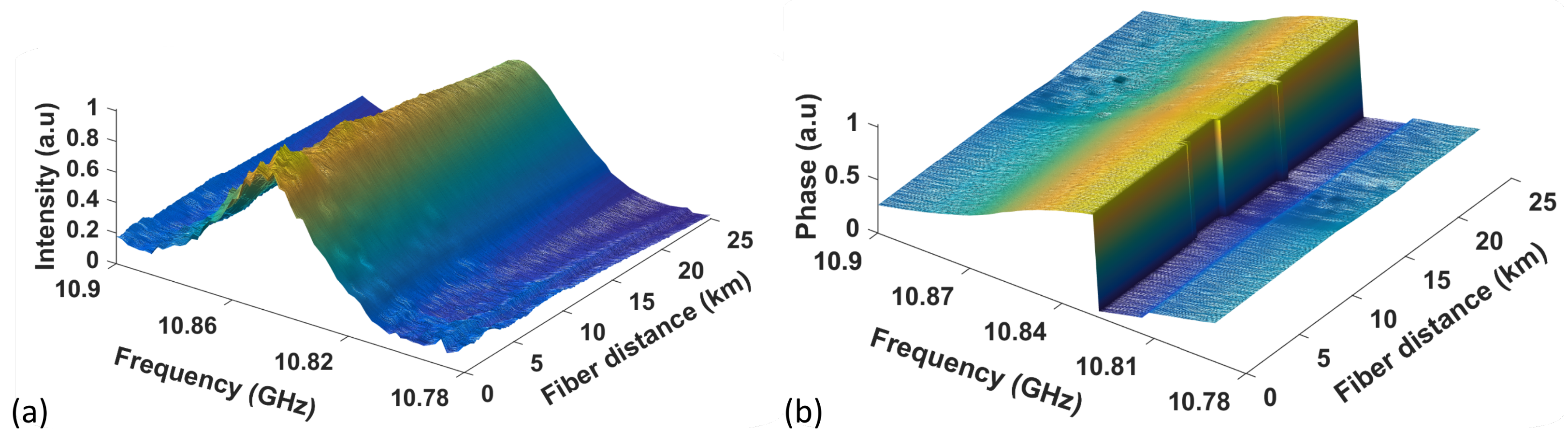
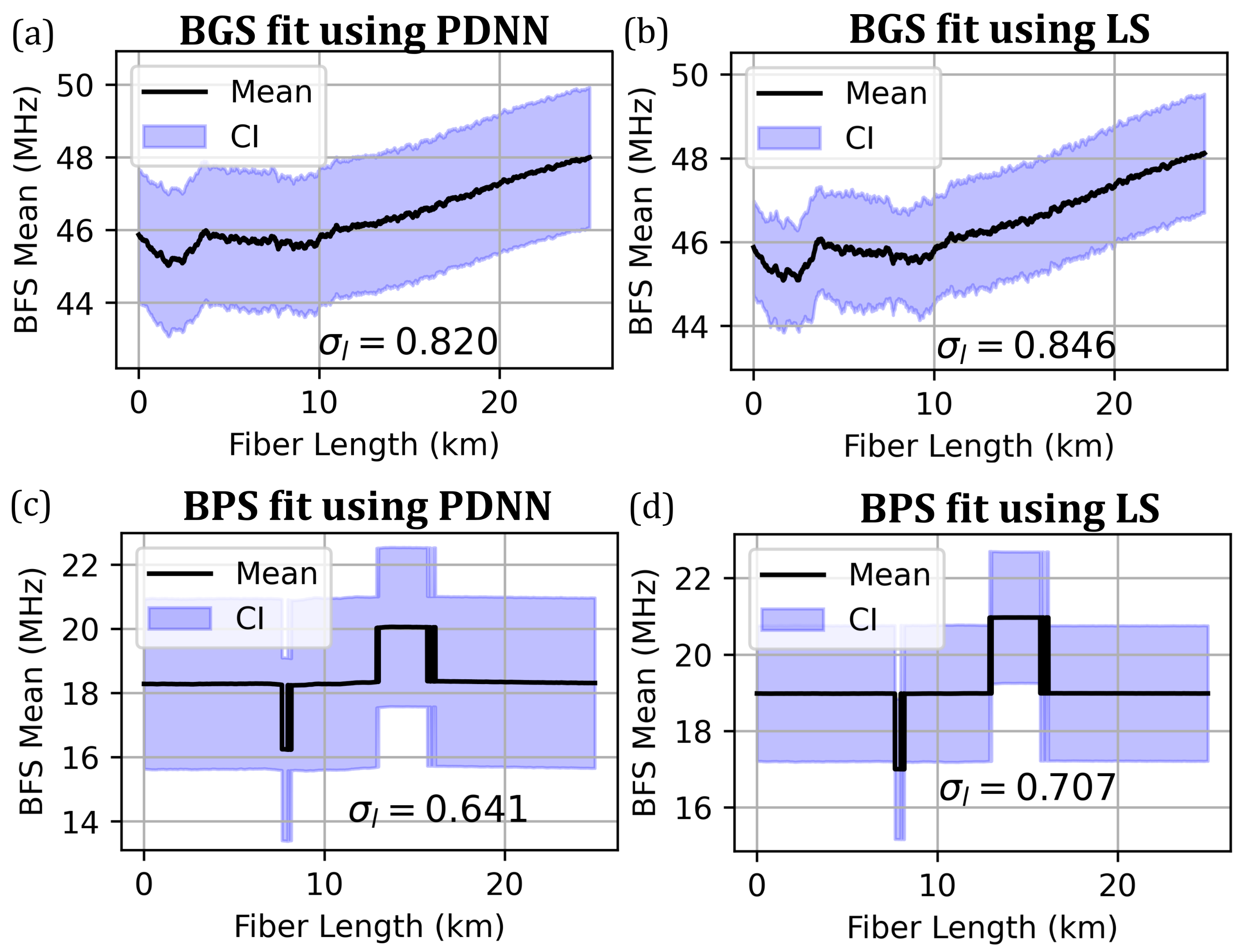
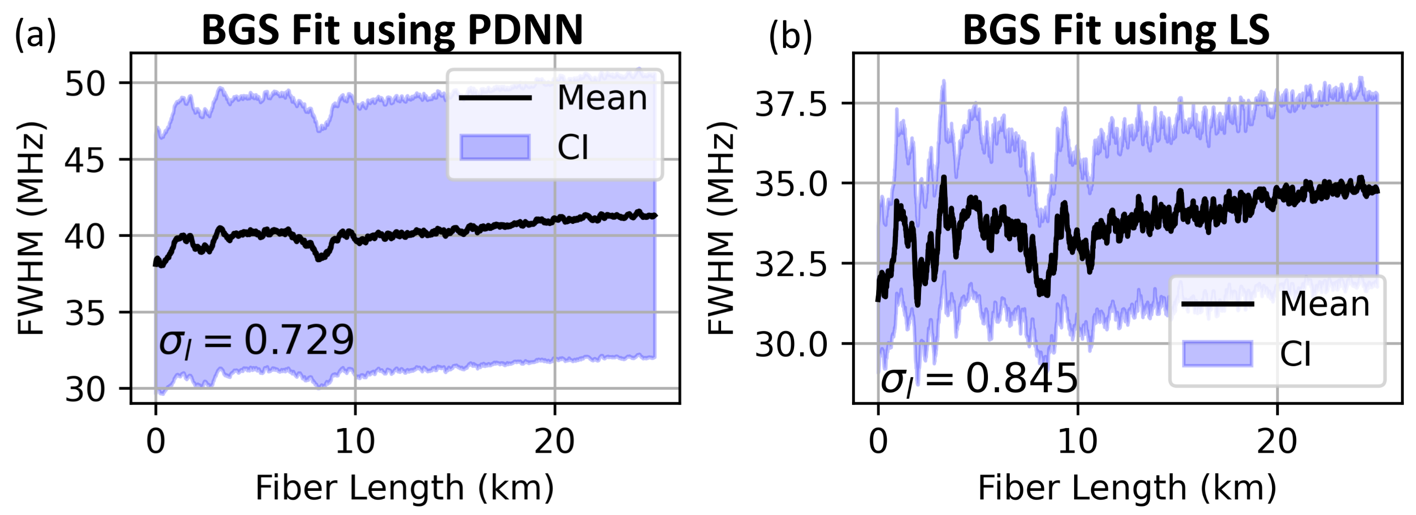
6.2. Custom VBOTDA System Using 25 km Long Sensing Fiber
7. Conclusions
Author Contributions
Funding
Data Availability Statement
Acknowledgments
Conflicts of Interest
References
- Bao, X.; Chen, L. Recent progress in Brillouin scattering based fiber sensors. Sensors 2011, 11, 4152–4187. [Google Scholar] [CrossRef] [PubMed]
- Lu, P.; Lalam, N.; Badar, M.; Liu, B.; Chorpening, B.T.; Buric, M.P.; Ohodnicki, P.R. Distributed optical fiber sensing: Review and perspective. Appl. Phys. Rev. 2019, 6, 041302. [Google Scholar] [CrossRef]
- Zhao, C.; Tang, M.; Wang, L.; Wu, H.; Zhao, Z.; Dang, Y.; Wu, J.; Fu, S.; Liu, D.; Shum, P.P. BOTDA using channel estimation with direct-detection optical OFDM technique. Opt. Express 2017, 25, 12698–12709. [Google Scholar] [CrossRef]
- He, H.; Yan, L.; Qian, H.; Li, Z.; Zhang, X.; Luo, B.; Pan, W. Efficient demodulation of Brillouin phase spectra and performance enhancement in BOTDA incorporating phase noise elimination. J. Light. Technol. 2019, 37, 4308–4314. [Google Scholar] [CrossRef]
- Li, Y.; An, Q.; Li, X.; Zhang, L. High-accuracy Brillouin frequency shift measurement system based on stimulated Brillouin scattering phase shift. Opt. Eng. 2017, 56, 056102. [Google Scholar] [CrossRef] [Green Version]
- Kadum, J.E.; Feng, C.; Schneider, T. Characterization of the Noise Induced by Stimulated Brillouin Scattering in Distributed Sensing. Sensors 2020, 20, 4311. [Google Scholar] [CrossRef] [PubMed]
- Tu, X.; Sun, Q.; Chen, W.; Chen, M.; Meng, Z. Vector Brillouin optical time-domain analysis with heterodyne detection and IQ demodulation algorithm. IEEE Photonics J. 2014, 6, 1–8. [Google Scholar] [CrossRef]
- Dossou, M.; Bacquet, D.; Szriftgiser, P. Vector Brillouin optical time-domain analyzer for high-order acoustic modes. Opt. Lett. 2010, 35, 3850–3852. [Google Scholar] [CrossRef] [Green Version]
- Lopez-Gil, A.; Soto, M.A.; Angulo-Vinuesa, X.; Dominguez-Lopez, A.; Martin-Lopez, S.; Thévenaz, L.; Gonzalez-Herraez, M. Evaluation of the accuracy of BOTDA systems based on the phase spectral response. Opt. Express 2016, 24, 17200–17214. [Google Scholar] [CrossRef]
- Lu, P.; Lalam, N.; Liu, B.; Buric, M.; Ohodnicki, P.R. Vector Brillouin optical time-domain analysis with Raman amplification and optical pulse coding. In Proceedings of the Photonic Instrumentation Engineering VI. International Society for Optics and Photonics, San Francisco, CA, USA, 5–7 February 2019; Volume 10925, p. 1092512. [Google Scholar]
- Wang, B.; Guo, N.; Wang, L.; Yu, C.; Lu, C. Robust and fast temperature extraction for Brillouin optical time-domain analyzer by using denoising autoencoder-based deep neural networks. IEEE Sens. J. 2019, 20, 3614–3620. [Google Scholar] [CrossRef]
- Venketeswaran, A.; Lalam, N.; Wuenschell, J.; Ohodnicki, P.R., Jr.; Badar, M.; Chen, K.P.; Lu, P.; Duan, Y.; Chorpening, B.; Buric, M. Recent Advances in Machine Learning for Fiber Optic Sensor Applications. Adv. Intell. Syst. 2021, 4, 2100067. [Google Scholar] [CrossRef]
- Lalam, N.; Ng, W.P.; Dai, X.; Wu, Q.; Fu, Y.Q. Performance improvement of Brillouin ring laser based BOTDR system employing a wavelength diversity technique. J. Light. Technol. 2018, 36, 1084–1090. [Google Scholar] [CrossRef] [Green Version]
- Urricelqui, J.; Soto, M.A.; Thévenaz, L. Sources of noise in Brillouin optical time-domain analyzers. In Proceedings of the 24th International Conference on Optical Fibre Sensors, SPIE, Curitiba, Brazil, 28 September–2 October 2015; Volume 9634, pp. 377–380. [Google Scholar]
- Zhang, Y.; Fu, G.; Liu, Y.; Bi, W.; Li, D. A novel fitting algorithm for Brillouin scattering spectrum of distributed sensing systems based on RBFN networks. Opt.-Int. J. Light Electron Opt. 2013, 124, 718–721. [Google Scholar] [CrossRef]
- Da Silva, L.C.B.; Samatelo, J.L.A.; Segatto, M.E.V.; Bazzo, J.P.; da Silva, J.C.C.; Martelli, C.; Pontes, M.J. NARX neural network model for strong resolution improvement in a distributed temperature sensor. Appl. Opt. 2018, 57, 5859–5864. [Google Scholar] [CrossRef]
- Wu, H.; Wang, L.; Guo, N.; Shu, C.; Lu, C. Support vector machine assisted BOTDA utilizing combined Brillouin gain and phase information for enhanced sensing accuracy. Opt. Express 2017, 25, 31210–31220. [Google Scholar] [CrossRef] [PubMed]
- Wang, B.; Wang, L.; Guo, N.; Zhao, Z.; Yu, C.; Lu, C. Deep neural networks assisted BOTDA for simultaneous temperature and strain measurement with enhanced accuracy. Opt. Express 2019, 27, 2530–2543. [Google Scholar] [CrossRef] [PubMed]
- Venketeswaran, A.; Lalam, N.; Lu, P.; Ohodnicki, P.R.; Chen, K.P. Enhanced Signal Processing of Distributed Brillouin Fiber Sensors using a Decoupled Radial Basis Function Network. In Proceedings of the Optical Fiber Sensors, Washington, DC, USA, 8–12 June 2020; Optica Publishing Group: Washington, DC, USA, 2020; p. T3-51. [Google Scholar]
- Lalam, N.; Lu, P.; Venketeswaran, A.; Buric, M.; Ohodnicki, P.R. Raman-assisted BOTDA performance improvement with the differential pulse-width pair technique and an artificial neural network based fitting algorithm. In Proceedings of the Autonomous Systems: Sensors, Processing, and Security for Vehicles and Infrastructure 2020, Virtual, 27 April–8 May 2020; International Society for Optics and Photonics: Bellingham, WA, USA, 2020; Volume 11415, p. 1141503. [Google Scholar]
- Soto, M.A.; Thévenaz, L. Modeling and evaluating the performance of Brillouin distributed optical fiber sensors. Opt. Express 2013, 21, 31347–31366. [Google Scholar] [CrossRef] [Green Version]
- Lakshminarayanan, B.; Pritzel, A.; Blundell, C. Simple and scalable predictive uncertainty estimation using deep ensembles. arXiv 2016, arXiv:1612.01474. [Google Scholar]
- Ovadia, Y.; Fertig, E.; Ren, J.; Nado, Z.; Sculley, D.; Nowozin, S.; Dillon, J.V.; Lakshminarayanan, B.; Snoek, J. Can you trust your model’s uncertainty? Evaluating predictive uncertainty under dataset shift. arXiv 2019, arXiv:1906.02530. [Google Scholar]
- Gal, Y. Uncertainty in Deep Learning. Ph.D. Thesis, University of Cambridge, Cambridge, UK, 2016. [Google Scholar]
- Xu, Z.; Zhao, L. Key parameter extraction for fiber Brillouin distributed sensors based on the exact model. Sensors 2018, 18, 2419. [Google Scholar] [CrossRef] [Green Version]
- Xu, Z.; Zhao, L.; Qin, H. Selection of spectrum model in estimation of Brillouin frequency shift for distributed optical fiber sensor. Optik 2019, 199, 163355. [Google Scholar] [CrossRef]
- Alem, M.; Soto, M.A.; Tur, M.; Thévenaz, L. Analytical expression and experimental validation of the Brillouin gain spectral broadening at any sensing spatial resolution. In Proceedings of the 2017 25th Optical Fiber Sensors Conference (OFS), Jeju Island, Republic of Korea, 24–28 April 2017; pp. 1–4. [Google Scholar]
- Lopez-Gil, A.; Angulo-Vinuesa, X.; Soto, M.A.; Dominguez-Lopez, A.; Martin-Lopez, S.; Thévenaz, L.; Gonzalez-Herraez, M. Gain vs phase in BOTDA setups. In Proceedings of the Sixth European Workshop on Optical Fibre Sensors. International Society for Optics and Photonics, Limerick, Ireland, 31 May–3 June 2016; Volume 9916, p. 991631. [Google Scholar]
- Seber, G.A.; Wild, C.J. Nonlinear Regression; John Wiley Sons: Hoboken, NJ, USA, 2003; Volume 62, p. 63. [Google Scholar]
- Azad, A.K.; Khan, F.N.; Alarashi, W.H.; Guo, N.; Lau, A.P.T.; Lu, C. Temperature extraction in Brillouin optical time-domain analysis sensors using principal component analysis based pattern recognition. Opt. Express 2017, 25, 16534–16549. [Google Scholar] [CrossRef]
- Azad, A.K.; Wang, L.; Guo, N.; Tam, H.Y.; Lu, C. Signal processing using artificial neural network for BOTDA sensor system. Opt. Express 2016, 24, 6769–6782. [Google Scholar] [CrossRef]
- Liehr, S. Artificial neural networks for distributed optical fiber sensing. In Proceedings of the Optical Fiber Communication Conference, Washington, DC, USA, 6–11 June 2021; Optical Society of America: Washington, DC, USA, 2021; p. Th4F-2. [Google Scholar]
- Wu, H.; Wan, Y.; Tang, M.; Chen, Y.; Zhao, C.; Liao, R.; Chang, Y.; Fu, S.; Shum, P.P.; Liu, D. Real-time denoising of Brillouin optical time domain analyzer with high data fidelity using convolutional neural networks. J. Light. Technol. 2019, 37, 2648–2653. [Google Scholar] [CrossRef]
- Zheng, H.; Yan, Y.; Wang, Y.; Sben, X.; Lu, C. Deep learning enhanced long-range fast BOTDA for vibration measurement. J. Light. Technol. 2021, 40, 262–268. [Google Scholar] [CrossRef]
- Kingma, D.P.; Welling, M. Auto-encoding variational bayes. arXiv 2013, arXiv:1312.6114. [Google Scholar]
- Srivastava, N.; Hinton, G.; Krizhevsky, A.; Sutskever, I.; Salakhutdinov, R. Dropout: A simple way to prevent neural networks from overfitting. J. Mach. Learn. Res. 2014, 15, 1929–1958. [Google Scholar]
- Efron, B. Bootstrap methods: Another look at the jackknife. In Breakthroughs in Statistics; Springer: Berlin/Heidelberg, Germany, 1992; pp. 569–593. [Google Scholar]
- Cao, W.; Wang, X.; Ming, Z.; Gao, J. A review on neural networks with random weights. Neurocomputing 2018, 275, 278–287. [Google Scholar] [CrossRef]
- Nix, D.A.; Weigend, A.S. Estimating the mean and variance of the target probability distribution. In Proceedings of the 1994 IEEE International Conference on Neural Networks (ICNN’94), Orlando, FL, USA, 28 June–2 July 1994; Volume 1, pp. 55–60. [Google Scholar]
- De Brabanter, K.; Karsmakers, P.; De Brabanter, J.; Suykens, J.A.; De Moor, B. Confidence bands for least squares support vector machine classifiers: A regression approach. Pattern Recognit. 2012, 45, 2280–2287. [Google Scholar] [CrossRef]
- Venketeswaran, A.; Lalam, N.; Lu, P.; Buric, M. Jupyter notebook containing the code for BFS and FWHM estimation using PDNN. Figshare. 2021. Available online: https://osapublishing.figshare.com/s/0fff0771379de177d5b3 (accessed on 9 May 2023).
- Chen, T.; Xu, X.; Lalam, N.; Ng, W.P.; Harrington, P. Multi point strain and temperature sensing based on Brillouin optical time domain reflectometry. In Proceedings of the 11th International Symposium on Communication Systems, Networks & Digital Signal Processing (CSNDSP), Budapest, Hungary, 18–20 July 2018; pp. 1–6. [Google Scholar]
- Muanenda, Y.; Taki, M.; Pasquale, F.D. Long-range accelerated BOTDA sensor using adaptive linear prediction and cyclic coding. Opt. Lett. 2014, 39, 5411–5414. [Google Scholar] [CrossRef]
- Venketeswaran, A.; Lalam, N.; Lu, P.; Buric, M. Dataset for gain spectra for 25km long fibre. Figshare. 2021. Available online: https://osapublishing.figshare.com/s/2e08c4082b7653f665fb (accessed on 9 May 2023).
- Venketeswaran, A.; Lalam, N.; Lu, P.; Buric, M. Dataset for phase spectra for 25km long fibre. Figshare. 2021. Available online: https://osapublishing.figshare.com/s/1ca66af63c3245a9c986 (accessed on 9 May 2023).


| Gain Spectrum | Function | Parameters |
|---|---|---|
| Lorentzian | ||
| Gaussian | ||
| Pseudo-Voigt |
Disclaimer/Publisher’s Note: The statements, opinions and data contained in all publications are solely those of the individual author(s) and contributor(s) and not of MDPI and/or the editor(s). MDPI and/or the editor(s) disclaim responsibility for any injury to people or property resulting from any ideas, methods, instructions or products referred to in the content. |
© 2023 by the authors. Licensee MDPI, Basel, Switzerland. This article is an open access article distributed under the terms and conditions of the Creative Commons Attribution (CC BY) license (https://creativecommons.org/licenses/by/4.0/).
Share and Cite
Venketeswaran, A.; Lalam, N.; Lu, P.; Bukka, S.R.; Buric, M.P.; Wright, R. Robust Vector BOTDA Signal Processing with Probabilistic Machine Learning. Sensors 2023, 23, 6064. https://doi.org/10.3390/s23136064
Venketeswaran A, Lalam N, Lu P, Bukka SR, Buric MP, Wright R. Robust Vector BOTDA Signal Processing with Probabilistic Machine Learning. Sensors. 2023; 23(13):6064. https://doi.org/10.3390/s23136064
Chicago/Turabian StyleVenketeswaran, Abhishek, Nageswara Lalam, Ping Lu, Sandeep R. Bukka, Michael P. Buric, and Ruishu Wright. 2023. "Robust Vector BOTDA Signal Processing with Probabilistic Machine Learning" Sensors 23, no. 13: 6064. https://doi.org/10.3390/s23136064