

Improved Performance for PMSM Sensorless Control Based on Robust-Type Controller, ESO-Type Observer, Multiple Neural Networks, and RL-TD3 Agent †

 ,
,  ,
,  and
and
Abstract
:1. Introduction
- The synthesis of a robust PMSM controller using the d-q frame mathematical model for the sensored case of the PMSM control structure;
- The robust controller synthesis using MATLAB and integration with PMSM sensored control system;
- The improvement in the control performance of the PMSM sensored control system, by combining the robust controller and an RL-TD3 agent that provides additional correction signals to adjust the ud and uq commands generated by the main robust controller;
- The comparative presentation of the performance of the proposed controllers used in the PMSM control system structure, in terms of response time, speed ripple error and DF of the rotor speed signal;
- The ESO-type observer synthesis for the sensorless case of the PMSM control system for rotor speed estimation;
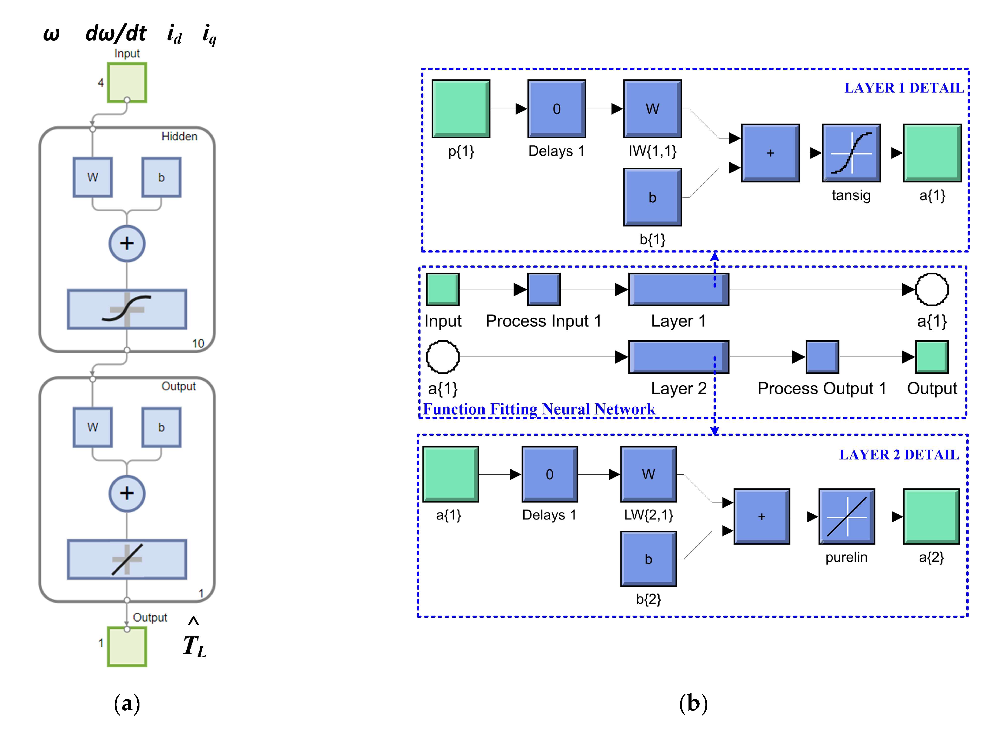
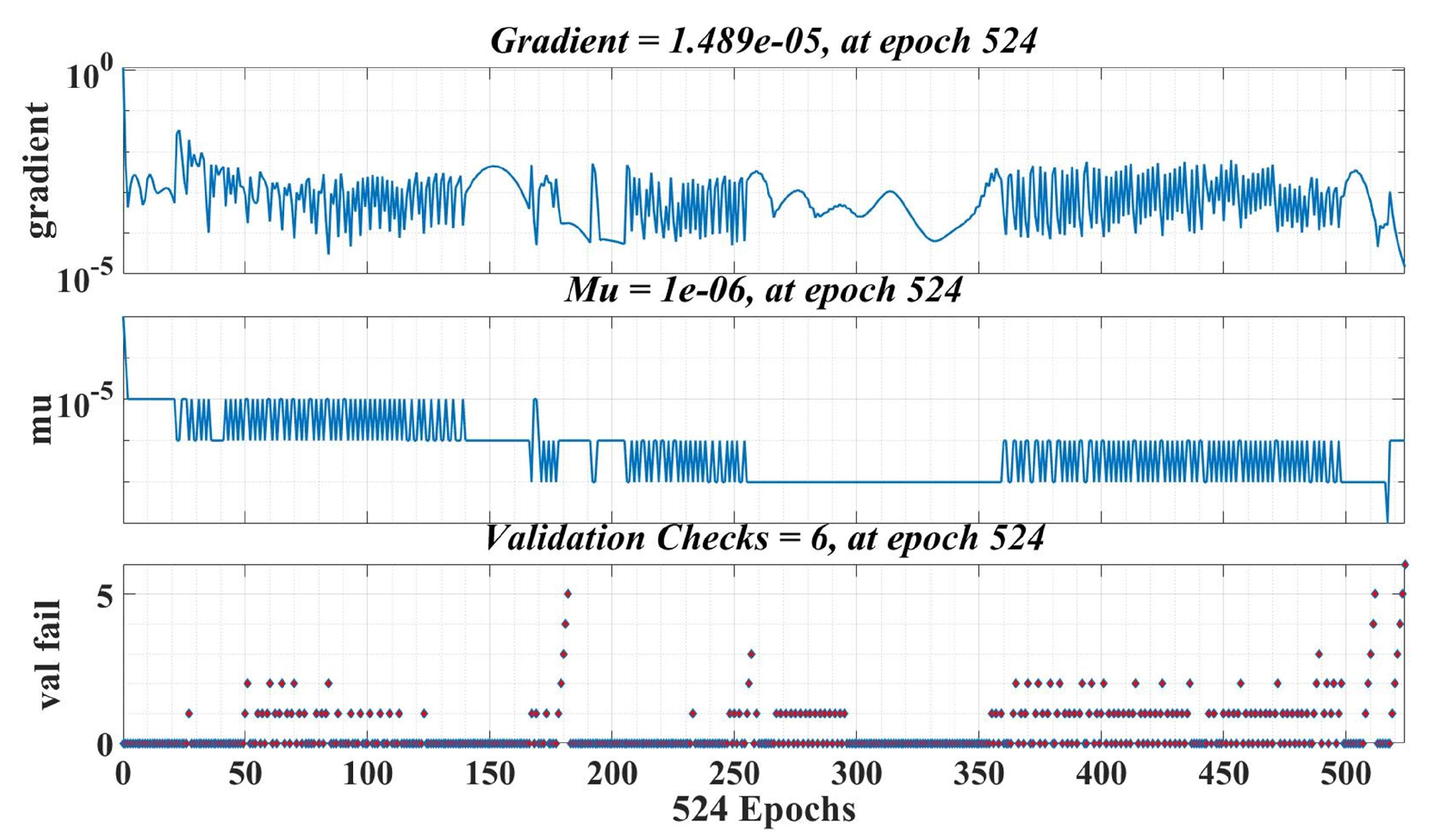
- The improvement in the performance of the basic ESO observer structure for PMSM rotor speed estimation, by providing load torque estimates using two-layer feed-forward multiple NN networks implemented with the Neural Net Fitting MATLAB application [31];
- The improvement in the performance of the ESO basic observer structure for PMSM rotor speed estimation, by implementing an RL-TD3 agent [33] in MATLAB/Simulink that provides correction signals to estimate the PMSM rotor speed value as close as possible to the sensored rotor speed provided by a PMSM speed sensor;
- Comparison of the performance of the four observer variants for estimating the proposed PMSM rotor speed, in terms of response time and speed ripple error.
2. Sensored and Sensorless PMSM Control
3. Robust Control of PMSM
4. MATLAB/Simulink Implementation and Numerical Simulations for PMSM Sensored Control System Using a Robust Controller Combined with RL-TD3 Agent
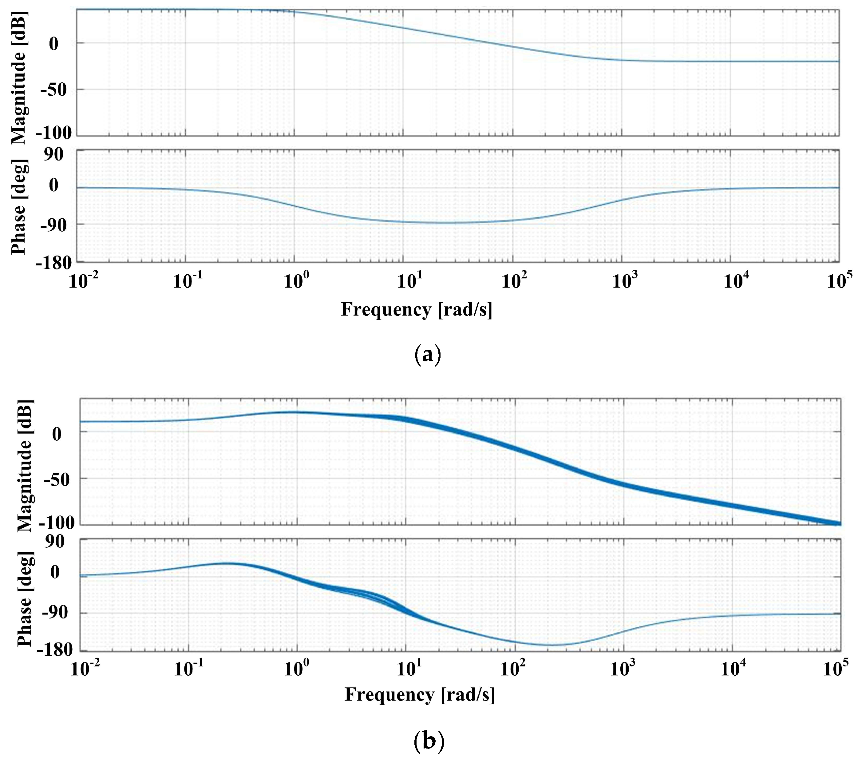
4.1. Robust Controller Synthesis Based on MATLAB/Simulink
4.2. Improvement in the Robust Control of PMSM Sensored Control System Using RL-TD3 Agent
5. PMSM Sensorless Control System Using Improved ESO-Type Observer Variants
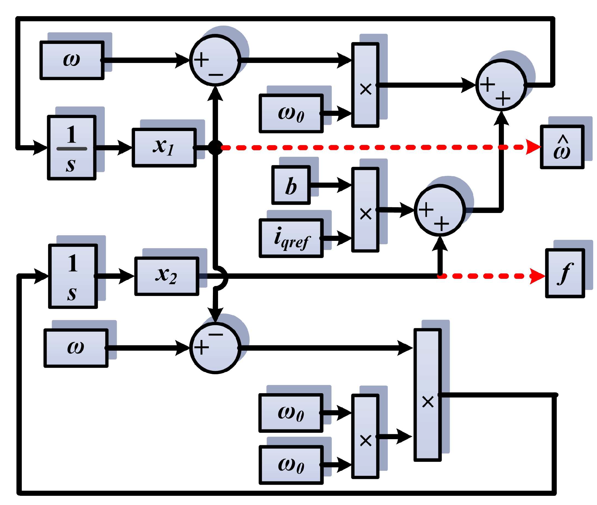
5.1. ESO-Type Observer Description
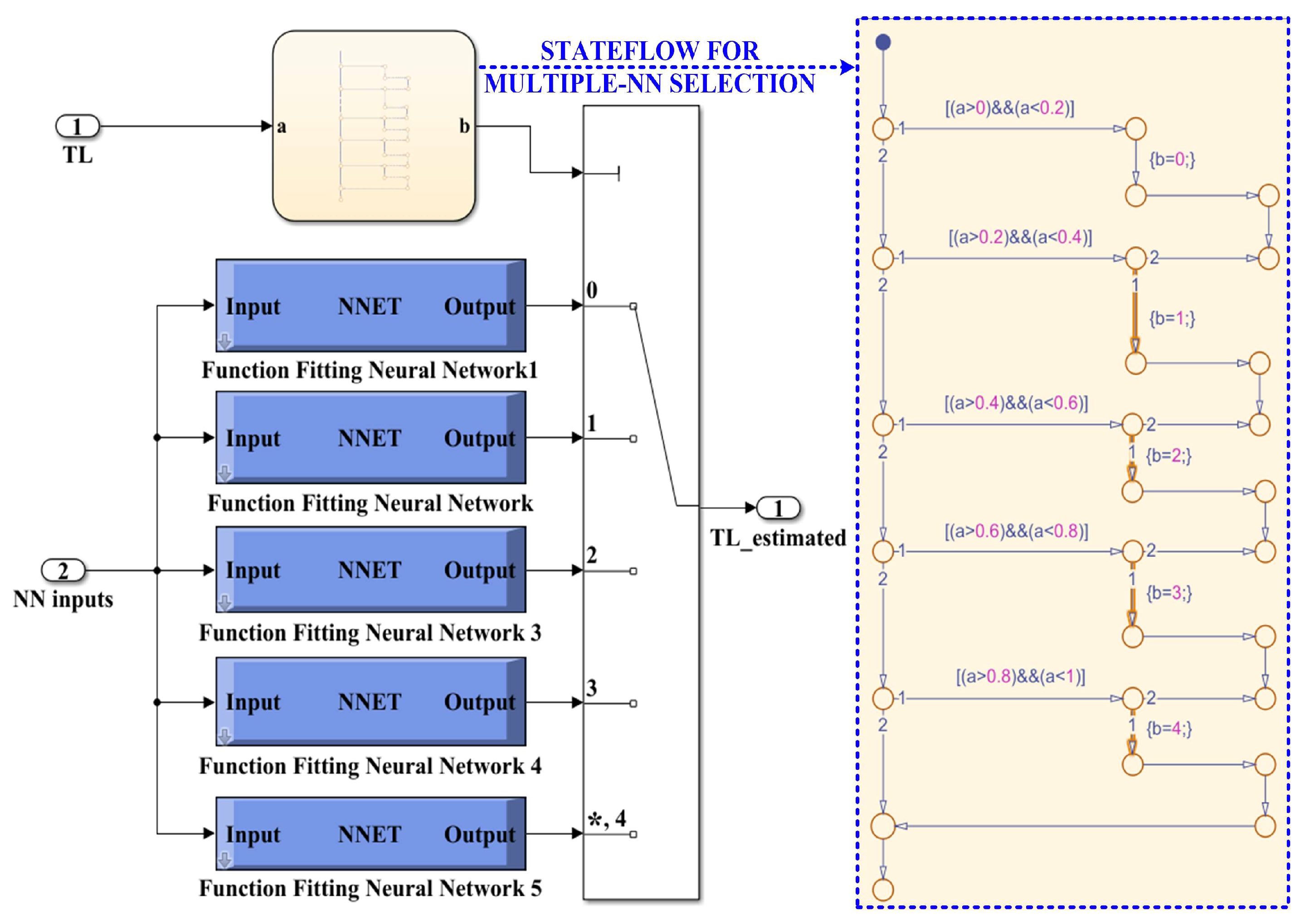
5.2. Load Torque Estimation Using Multiple NN
5.3. Improved Estimation of PMSM Rotor Speed Using ESO-Type Observer and RL-TD3 Agent
6. Numerical Simulation of the PMSM Sensorless Control System
7. Conclusions
Author Contributions
Funding
Institutional Review Board Statement
Informed Consent Statement
Data Availability Statement
Conflicts of Interest
References
- Krishnan, R. Permanent Magnet Synchronous and Brushless DC Motor Drives; CRC Press/Taylor & Francis: Boca Raton, FL, USA, 2017. [Google Scholar]
- Bose, B.K. Modern Power Electronics and AC Drives; Prentice Hall PTR: Hoboken, NJ, USA, 2002. [Google Scholar]
- Zhang, X.; Wang, C.; Wang, T.; Wang, G.; Song, Z.; Huang, J. Research on the control strategy of five-phase fault-tolerant servo system for aerospace. In Proceedings of the CSAA/IET International Conference on Aircraft Utility Systems (AUS 2020), Online, 18–21 September 2020; pp. 1090–1094. [Google Scholar]
- Lekshmi, S.; Lal Priya, P.S. Range Extension of Electric Vehicles with Independently Driven Front and Rear PMSM Drives by Optimal Driving and Braking Torque Distribution. In Proceedings of the IEEE International Conference on Power Electronics, Smart Grid and Renewable Energy (PESGRE2020), Cochin, India, 2–4 January 2020; pp. 1–6. [Google Scholar]
- Golesorkhie, F.; Yang, F.; Vlacic, L.; Tansley, G. Field Oriented Control-Based Reduction of the Vibration and Power Consumption of a Blood Pump. Energies 2020, 13, 3907. [Google Scholar] [CrossRef]
- Tang, X.; Zhang, Z.; Liu, X.; Liu, C.; Jiang, M.; Song, Y. A Novel Field-Oriented Control Algorithm for Permanent Magnet Synchronous Motors in 60° Coordinate Systems. Actuators 2023, 12, 92. [Google Scholar] [CrossRef]
- Guo, J.; Fan, T.; Li, Q.; Wen, X. An Angle-Compensating, Complex-Coefficient PI Controller Used for Decoupling Control of a Permanent-Magnet Synchronous Motor. Symmetry 2022, 14, 101. [Google Scholar] [CrossRef]
- Wei, Z.; Zhao, M.; Liu, X.; Lu, M. A Novel Variable-Proportion Desaturation PI Control for Speed Regulation in Sensorless PMSM Drive System. Appl. Sci. 2022, 12, 9234. [Google Scholar] [CrossRef]
- Huang, Y.; Zhang, J.; Chen, D.; Qi, J. Model Reference Adaptive Control of Marine Permanent Magnet Propulsion Motor Based on Parameter Identification. Electronics 2022, 11, 1012. [Google Scholar] [CrossRef]
- Vujji, A.; Dahiya, R. Speed Estimator for Direct Torque and Flux Control of PMSM Drive using MRAC based on Rotor flux. In Proceedings of the IEEE 9th Power India International Conference (PIICON), Sonepat, India, 28 February–1 March 2020; pp. 1–6. [Google Scholar]
- Park, J.-H.; Lim, H.-S.; Lee, G.-H.; Lee, H.-H. A Study on the Optimal Control of Voltage Utilization for Improving the Efficiency of PMSM. Electronics 2022, 11, 2095. [Google Scholar] [CrossRef]
- Nicola, M.; Nicola, C.-I. Improvement of Linear and Nonlinear Control for PMSM Using Computational Intelligence and Reinforcement Learning. Mathematics 2022, 10, 4667. [Google Scholar] [CrossRef]
- Wang, Y.; Li, H.; Yang, L.; Wang, X. Modulated Model-Free Predictive Control with Minimum Switching Losses for PMSM Drive System. IEEE Access 2020, 8, 20942–20953. [Google Scholar] [CrossRef]
- Zhou, C.; Yu, F.; Zhu, C.; Mao, J. Sensorless Predictive Current Control of a Permanent Magnet Synchronous Motor Powered by a Three-Level Inverter. Appl. Sci. 2021, 11, 10840. [Google Scholar] [CrossRef]
- Kakouche, K.; Rekioua, T.; Mezani, S.; Oubelaid, A.; Rekioua, D.; Blazek, V.; Prokop, L.; Misak, S.; Bajaj, M.; Ghoneim, S.S.M. Model Predictive Direct Torque Control and Fuzzy Logic Energy Management for Multi Power Source Electric Vehicles. Sensors 2022, 22, 5669. [Google Scholar] [CrossRef]
- Masoud, U.M.M.; Tiwari, P.; Gupta, N. Designing of an Enhanced Fuzzy Logic Controller of an Interior Permanent Magnet Synchronous Generator under Variable Wind Speed. Sensors 2023, 23, 3628. [Google Scholar] [CrossRef]
- Regaya, C.B.; Farhani, F.; Zaafouri, A.; Chaari, A. Adaptive Proportional-Integral Fuzzy Logic Controller of Electric Motor Drive. Eng. Rev. 2021, 42, 26–40. [Google Scholar] [CrossRef]
- Hoai, H.-K.; Chen, S.-C.; Chang, C.-F. Realization of the Neural Fuzzy Controller for the Sensorless PMSM Drive Control System. Electronics 2020, 9, 1371. [Google Scholar] [CrossRef]
- Farhani, F.; Regaya, C.B.; Zaafouri, A.; Chaari, A. Real Time PI-Backstepping Induction Machine Drive with Efficiency optimization. ISA Trans. 2017, 70, 348–356. [Google Scholar] [CrossRef] [PubMed]
- Zhu, Y.; Tao, B.; Xiao, M.; Yang, G.; Zhang, X.; Lu, K. Luenberger Position Observer Based on Deadbeat-Current Predictive Control for Sensorless PMSM. Electronics 2020, 9, 1325. [Google Scholar] [CrossRef]
- Gao, W.; Zhang, G.; Hang, M.; Cheng, S.; Li, P. Sensorless Control Strategy of a Permanent Magnet Synchronous Motor Based on an Improved Sliding Mode Observer. World Electr. Veh. J. 2021, 12, 74. [Google Scholar] [CrossRef]
- Comanescu, M.; Xu, L. Sliding-mode MRAS speed estimators for sensorless vector control of induction Machine. IEEE Trans. Ind. Electron. 2006, 53, 146–153. [Google Scholar] [CrossRef]
- Urbanski, K.; Janiszewski, D. Sensorless Control of the Permanent Magnet Synchronous Motor. Sensors 2019, 19, 3546. [Google Scholar] [CrossRef] [Green Version]
- Gu, D.-W.; Petkov, P.H.; Konstantinov, M.M. Robust Control Design with MATLAB (Advanced Textbooks in Control and Signal Processing), 2nd ed.; Springer: Berlin/Heidelberg, Germany, 2013. [Google Scholar]
- Cai, R.; Zheng, R.; Liu, M.; Li, M. Robust Control of PMSM Using Geometric Model Reduction and μ-Synthesis. IEEE Trans. Ind. Electron. 2018, 65, 498–509. [Google Scholar] [CrossRef]
- MathWorks—Robust Control Toolbox. Available online: https://www.mathworks.com/products/robust.html (accessed on 23 November 2021).
- Mendoza-Mondragón, F.; Hernández-Guzmán, V.M.; Rodríguez-Reséndiz, J. Robust Speed Control of Permanent Magnet Synchronous Motors Using Two-Degrees-of-Freedom Control. IEEE Trans. Ind. Electron. 2018, 65, 6099–6108. [Google Scholar] [CrossRef]
- Nicola, M.; Nicola, C.-I.; Ionete, C.; Șendrescu, D.; Roman. Improved Performance for PMSM Control Based on Robust Controller and Reinforcement Learning. In Proceedings of the 26th International Conference on System Theory, Control and Computing (ICSTCC), Sinaia, Romania, 19–21 October 2022; pp. 207–212. [Google Scholar]
- Nicola, C.-I.; Nicola, M.; Selișteanu, D. Sensorless Control of PMSM Based on Backstepping-PSO-Type Controller and ESO-Type Observer Using Real-Time Hardware. Electronics 2021, 10, 2080. [Google Scholar] [CrossRef]
- Nicola, M.; Nicola, C.-I.; Duţă, M. Sensorless Control of PMSM using FOC Strategy Based on Multiple ANN and Load Torque Observer. In Proceedings of the International Conference on Development and Application Systems (DAS), Suceava, Romania, 21–23 May 2020; pp. 32–37. [Google Scholar]
- MathWorks—Deep Learning Toolbox—Neural Net Fitting. Available online: https://www.mathworks.com/help/deeplearning/neuralnetfitting-app.html (accessed on 20 April 2020).
- Nicola, M.; Nicola, C.-I. Improvement of PMSM Control Using Reinforcement Learning Deep Deterministic Policy Gradient Agent. In Proceedings of the 21st International Symposium on Power Electronics (Ee), Novi Sad, Serbia, 27–30 October 2021; pp. 1–6. [Google Scholar]
- MathWorks—Twin-Delayed Deep Deterministic Policy Gradient Reinforcement Learning Agent. Available online: https://www.mathworks.com/help/reinforcement-learning/ug/td3-agents.html (accessed on 12 September 2021).
- Nicola, M.; Nicola, C.-I.; Sacerdoțianu, D.; Vintilă, A. Comparative Performance of UPQC Control System Based on PI-GWO, Fractional Order Controllers, and Reinforcement Learning Agent. Electronics 2023, 12, 494. [Google Scholar] [CrossRef]


| Parameter | Value | Unit |
|---|---|---|
| Stator resistance—Rs | 2.875 | Ω |
| Inductances on d-q rotating reference frame—Ld and Lq | 0.0085 | H |
| Combined inertia of rotor and load—J | 0.008 | kg·m2 |
| Combined viscous friction of rotor and load—B | 0.005 | N·m·s/rad |
| Flux induced by the permanent magnets of the rotor in the stator phases—λ0 | 0.175 | Wb |
| PMSM Pole pairs number—nP | 4 | - |
| Controller Used in PMSM Sensored Control System | Response Time [ms] | Rotor Speed Ripple [rpm] | DF of Rotor Speed Signal |
|---|---|---|---|
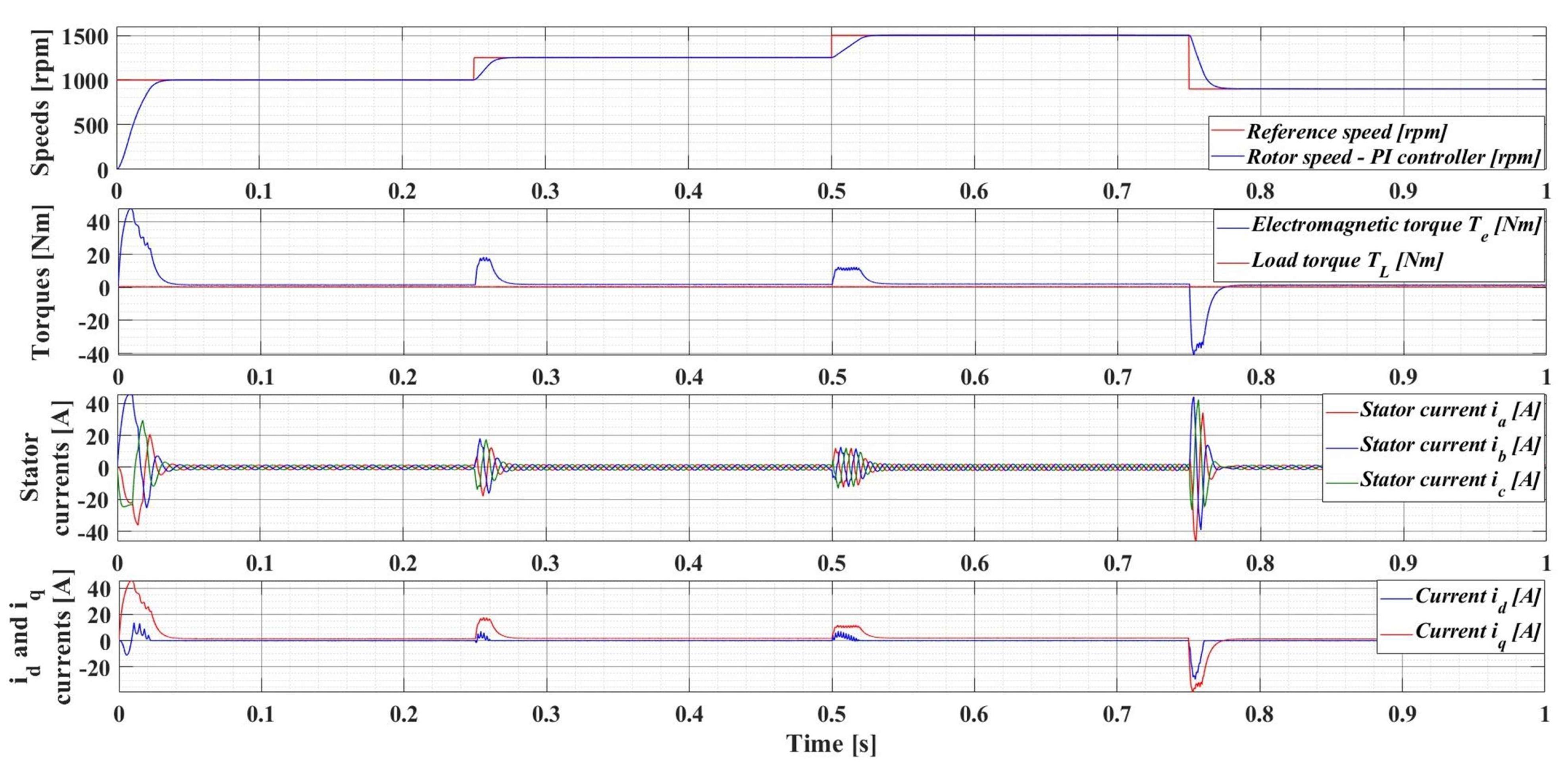
| PI controller | 30.1 | 108.1 | 0.95548 +/− 0.118370 |
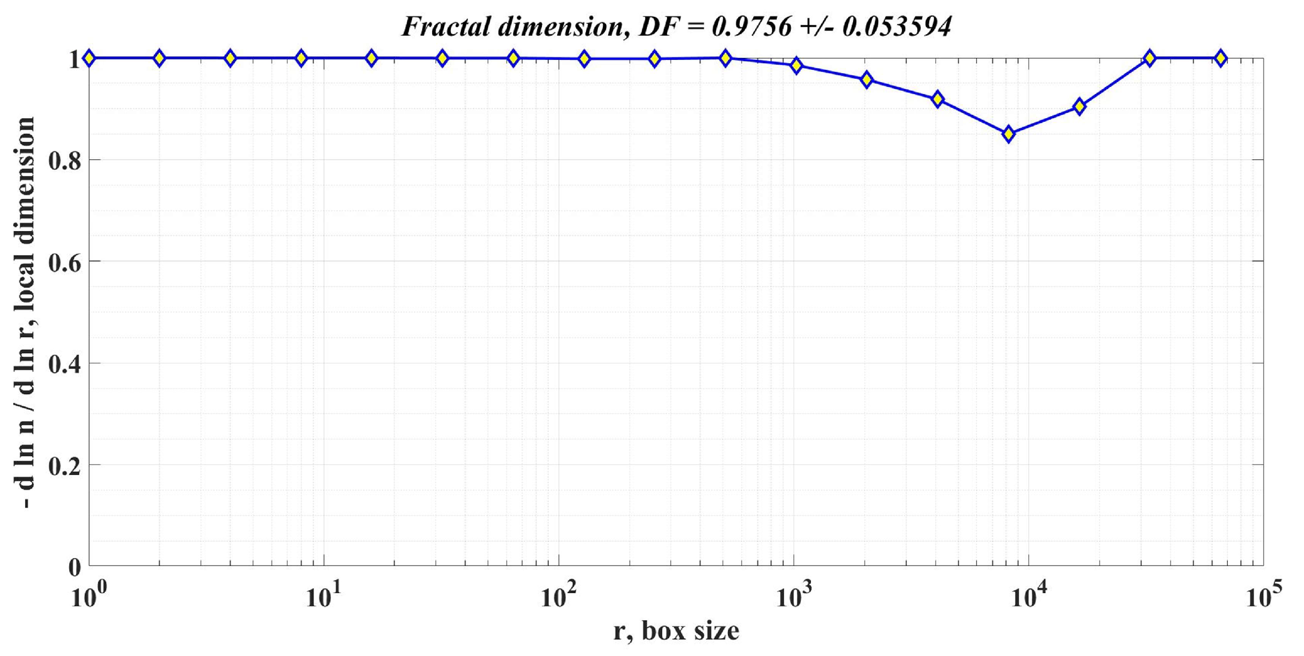
| Robust controller | 22.9 | 87.3 | 0.97560 +/− 0.053594 |
| Robust controller combined with RL-TD3 agent | 18.2 | 52.4 | 0.99204 +/− 0.023511 |
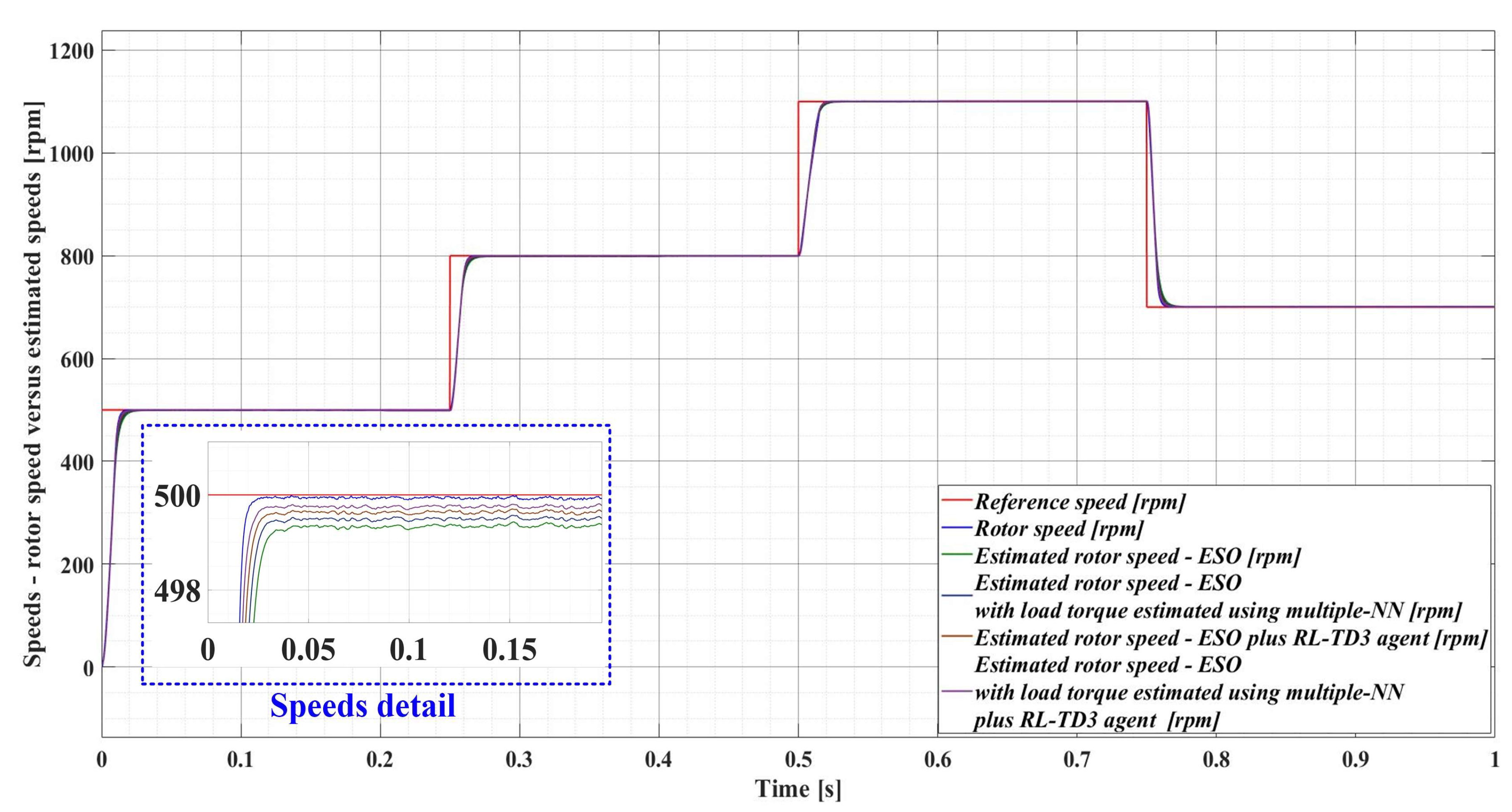
| Observer | Response Time [ms] | Improved of Response Time in Comparison with ESO-Type Basic Version Observer [%] | Estimated Speed Ripple [rpm] | Improved of Speed Ripple in Comparison with ESO-Type Basic Version Observer [%] |
|---|---|---|---|---|
| ESO-type basic version observer | 30.7 | – | 3.43 | – |
| ESO-type version observer with load torque estimated using multiple NN observer | 27.4 | 11 | 2.48 | 27 |
| ESO-type version observer combined RL-TD3 agent | 23.5 | 24 | 1.85 | 46 |
| ESO-type version observer with load torque estimated using multiple NN observer combined with RL-TD3 agent | 21.1 | 32 | 1.39 | 59 |
Disclaimer/Publisher’s Note: The statements, opinions and data contained in all publications are solely those of the individual author(s) and contributor(s) and not of MDPI and/or the editor(s). MDPI and/or the editor(s) disclaim responsibility for any injury to people or property resulting from any ideas, methods, instructions or products referred to in the content. |
© 2023 by the authors. Licensee MDPI, Basel, Switzerland. This article is an open access article distributed under the terms and conditions of the Creative Commons Attribution (CC BY) license (https://creativecommons.org/licenses/by/4.0/).
Share and Cite
Nicola, M.; Nicola, C.-I.; Ionete, C.; Șendrescu, D.; Roman, M. Improved Performance for PMSM Sensorless Control Based on Robust-Type Controller, ESO-Type Observer, Multiple Neural Networks, and RL-TD3 Agent. Sensors 2023, 23, 5799. https://doi.org/10.3390/s23135799
Nicola M, Nicola C-I, Ionete C, Șendrescu D, Roman M. Improved Performance for PMSM Sensorless Control Based on Robust-Type Controller, ESO-Type Observer, Multiple Neural Networks, and RL-TD3 Agent. Sensors. 2023; 23(13):5799. https://doi.org/10.3390/s23135799
Chicago/Turabian StyleNicola, Marcel, Claudiu-Ionel Nicola, Cosmin Ionete, Dorin Șendrescu, and Monica Roman. 2023. "Improved Performance for PMSM Sensorless Control Based on Robust-Type Controller, ESO-Type Observer, Multiple Neural Networks, and RL-TD3 Agent" Sensors 23, no. 13: 5799. https://doi.org/10.3390/s23135799