
A Comparative Study of Smart THD-Based Fault Protection Techniques for Distribution Networks


Abstract
:1. Introduction
- −
- The MSOGI-THD and SOGI-THD protection methods are explained and modeled using Matlab/Simulink to automatically detect symmetrical and unsymmetrical fault events in DSs;
- −
- A robust fault detection algorithm for the SOGI-THD is proposed. This approach increases the system’s reliability and accuracy and speeds up the protection system’s response in the event of a fault, regardless of the harmonics present in the grid before the fault. This approach is also computationally efficient;
- −
- A finite state machine has been used to locate and isolate faults in different locations, detect permanent faults, and ignore temporary faults;
- −
- A comparison study between the two THD-based approaches and the conventional methods is proposed under various conditions, such as changing the fault types, DG penetration, fault resistances, and fault locations in the network. Moreover, the study assesses the robustness of these methods against communication delays and the presence of harmonics before fault events. Additionally, the paper evaluates the computational burden of the different THD methods when implemented on a digital processor.
2. THD Measurement Methods
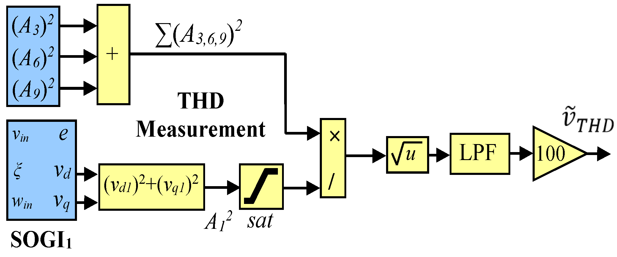
2.1. MSOGI-THD
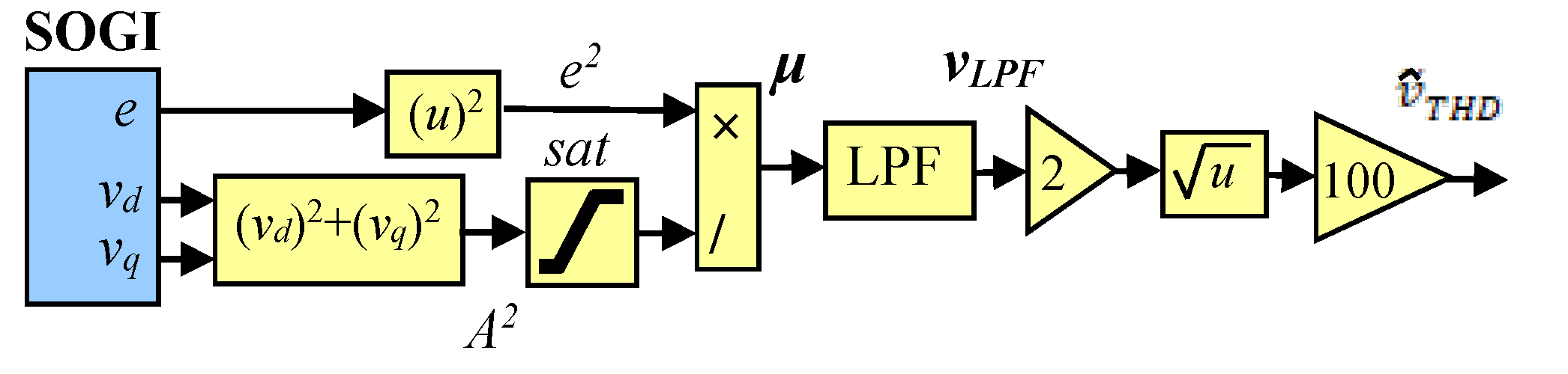
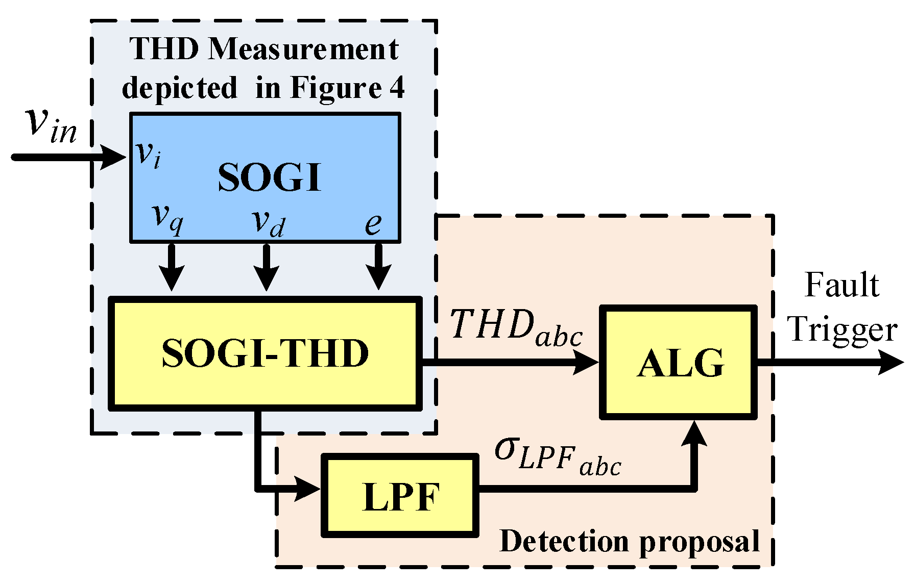
2.2. SOGI-THD
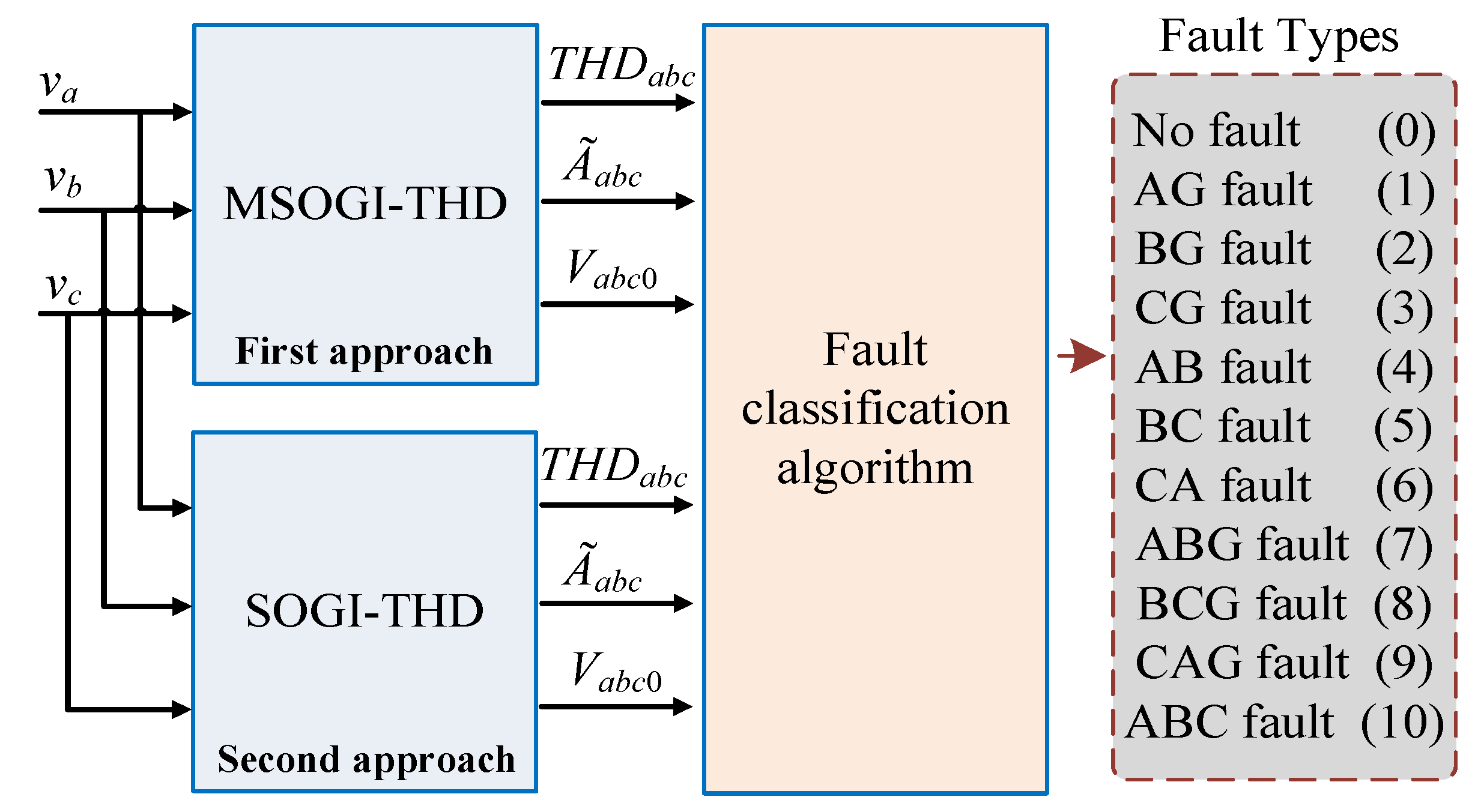
3. Fault Classification Algorithm
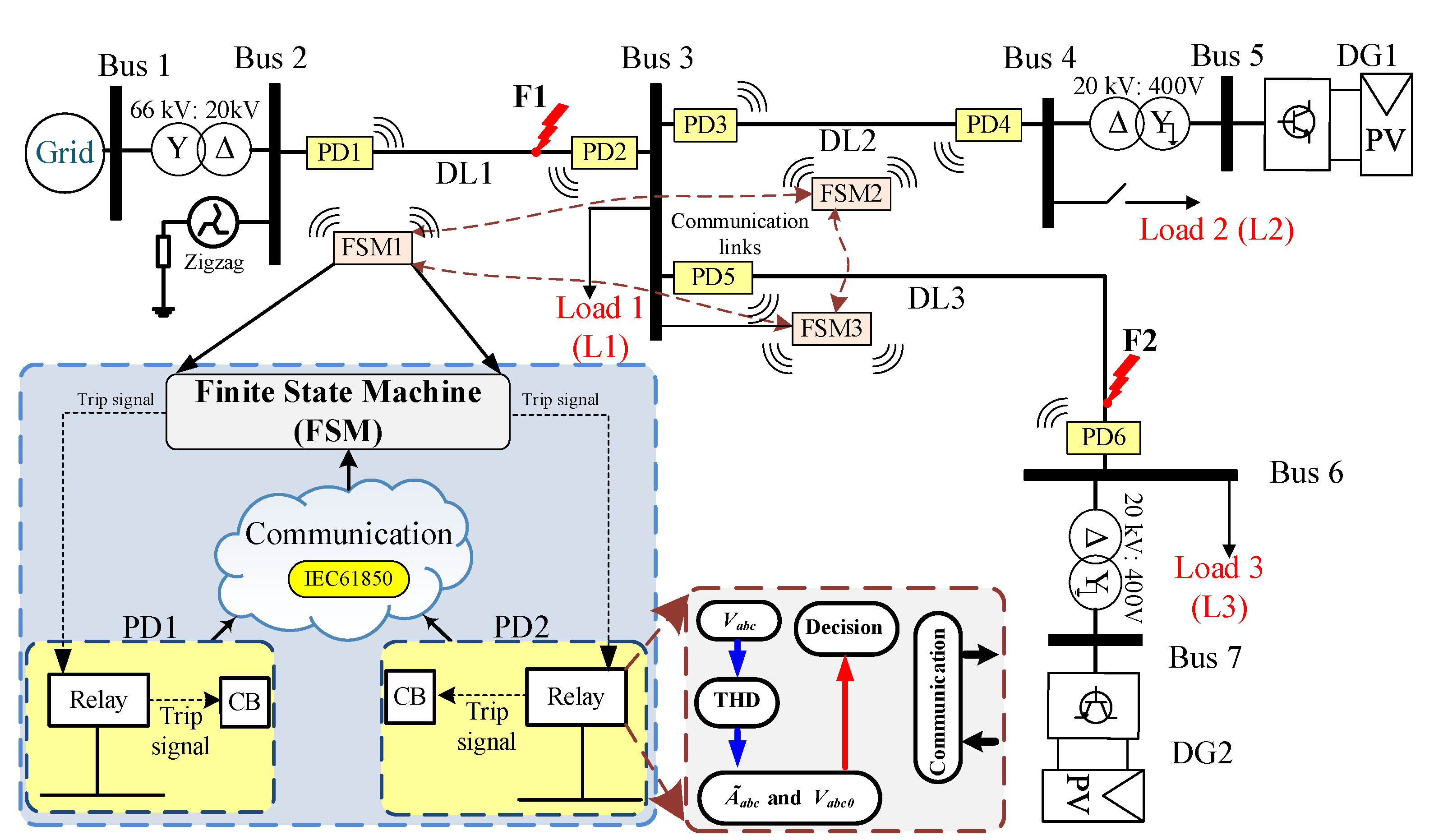
3.1. Proposed System
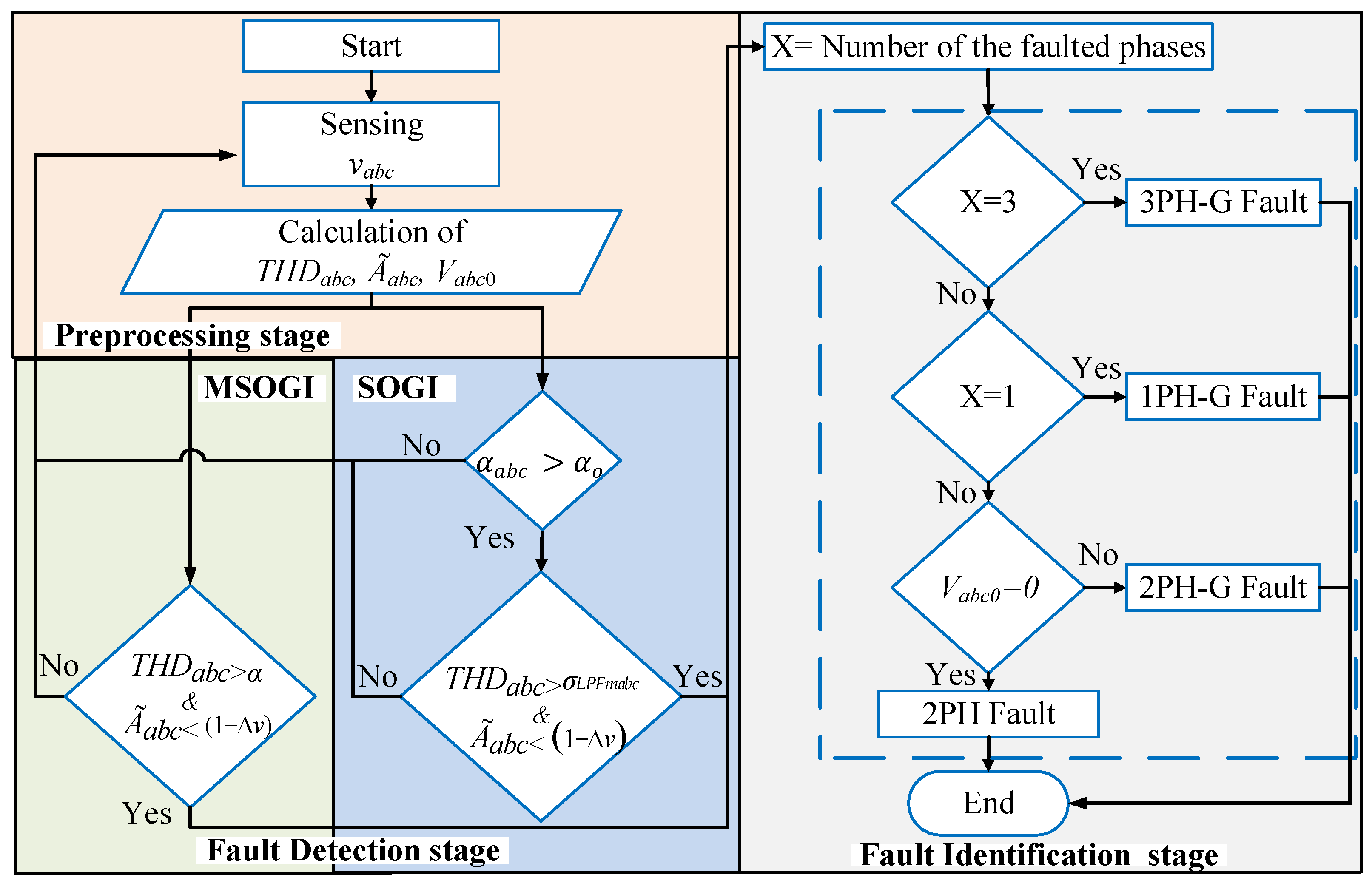
3.2. Fault Classification Algorithm Stages
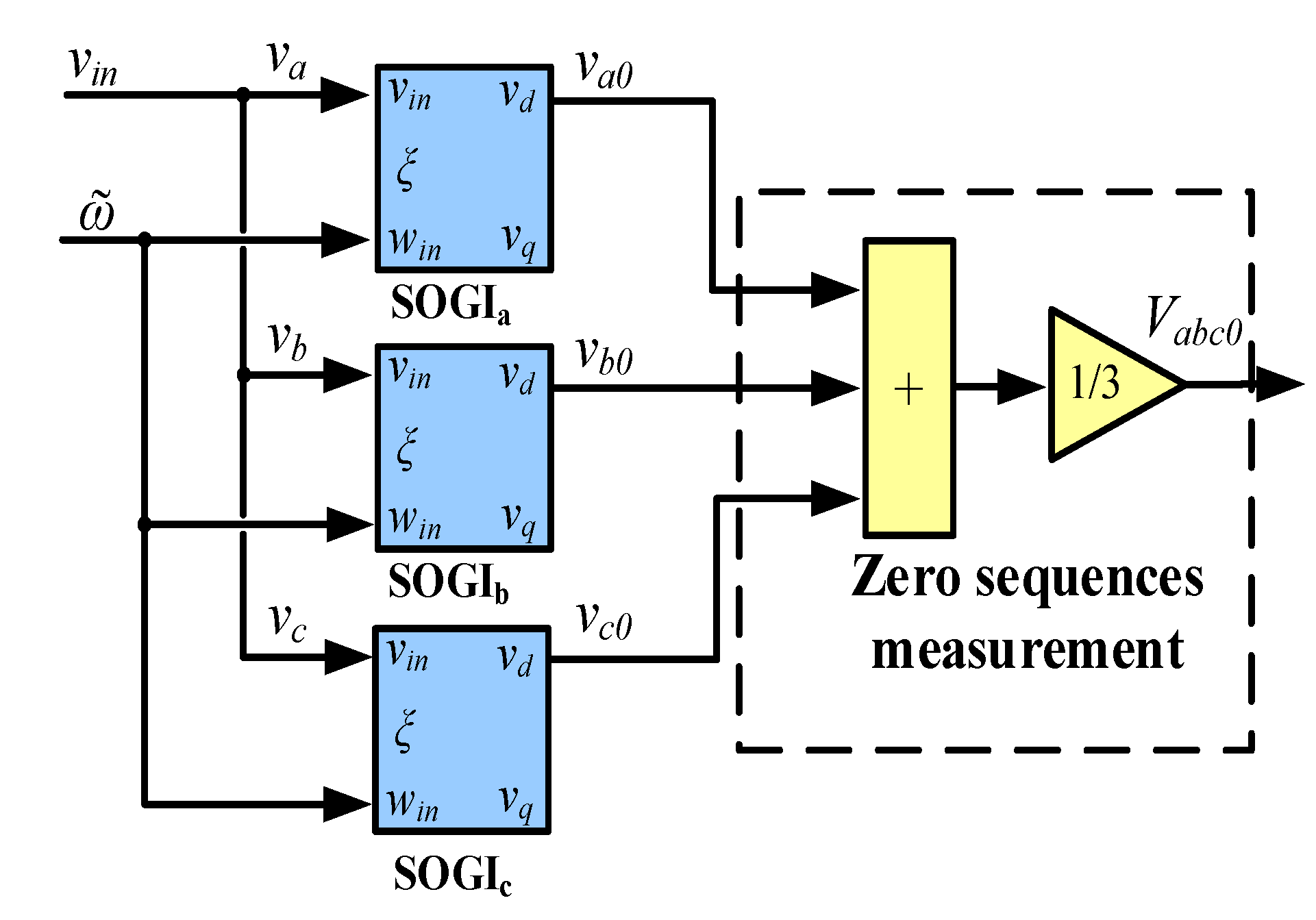
3.2.1. Pre-Processing Stage
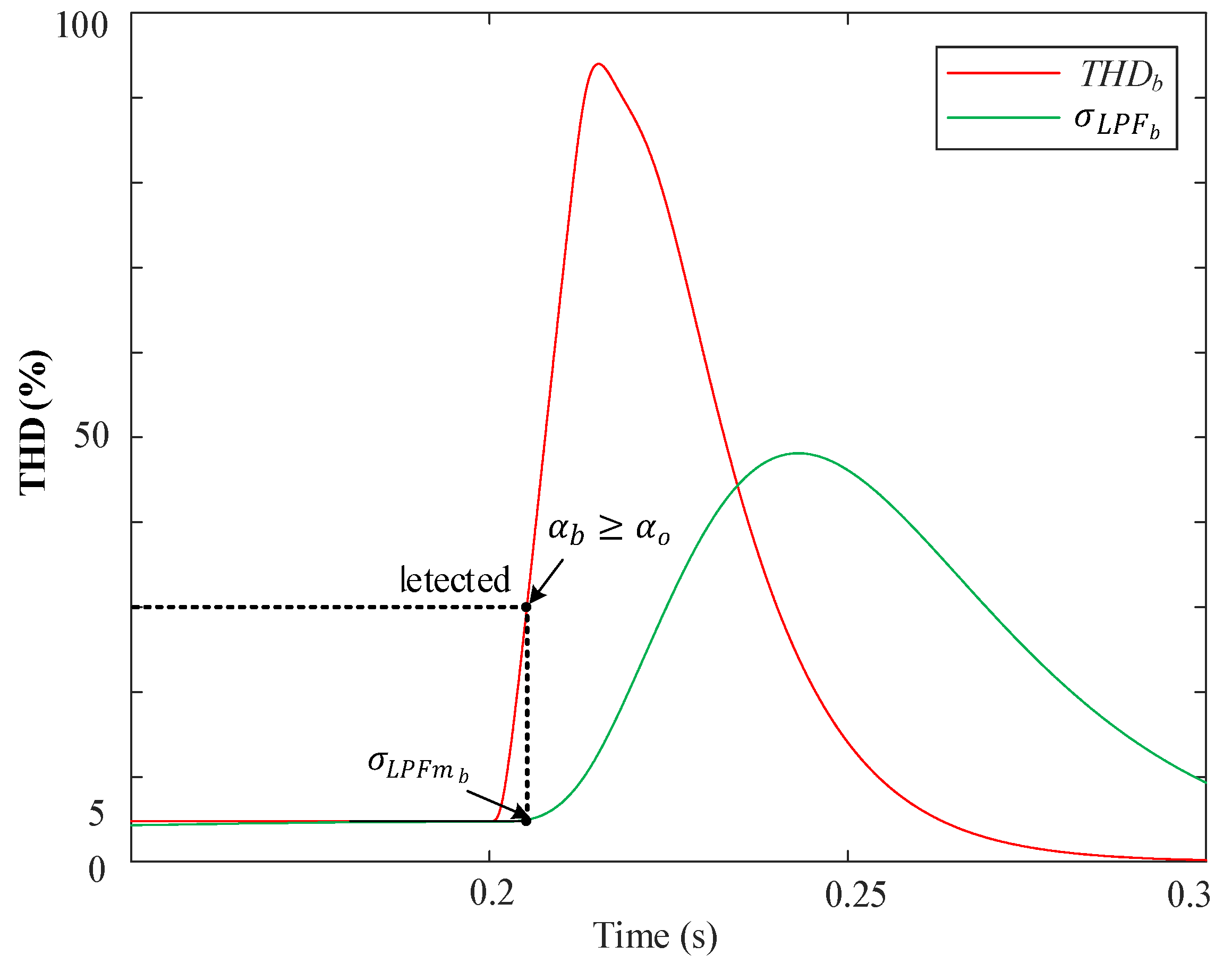
3.2.2. Fault Detection Stage
- MSOGI-THD
- 2.
- SOGI-THD
3.2.3. Fault Identification Stage
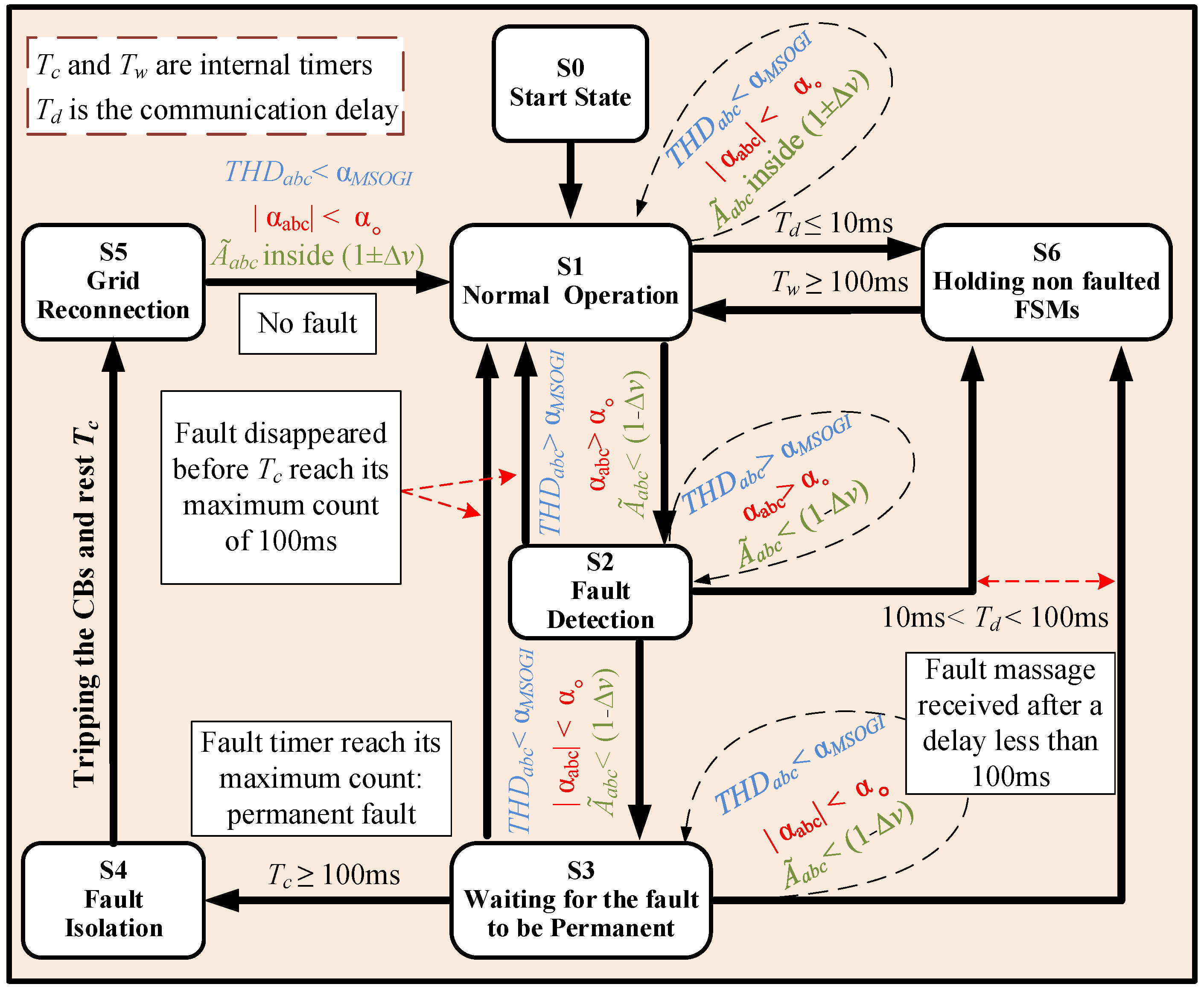
4. Finite State Machine
4.1. State S1: Normal Operation
4.2. State S2: Fault Detection
4.3. State S3: Waiting for the Fault to Be Permanent
4.4. State S4: Fault Isolation
4.5. State S5: Grid Reconnection
4.6. State S6: Holding Non-Faulted FSMs
5. Results
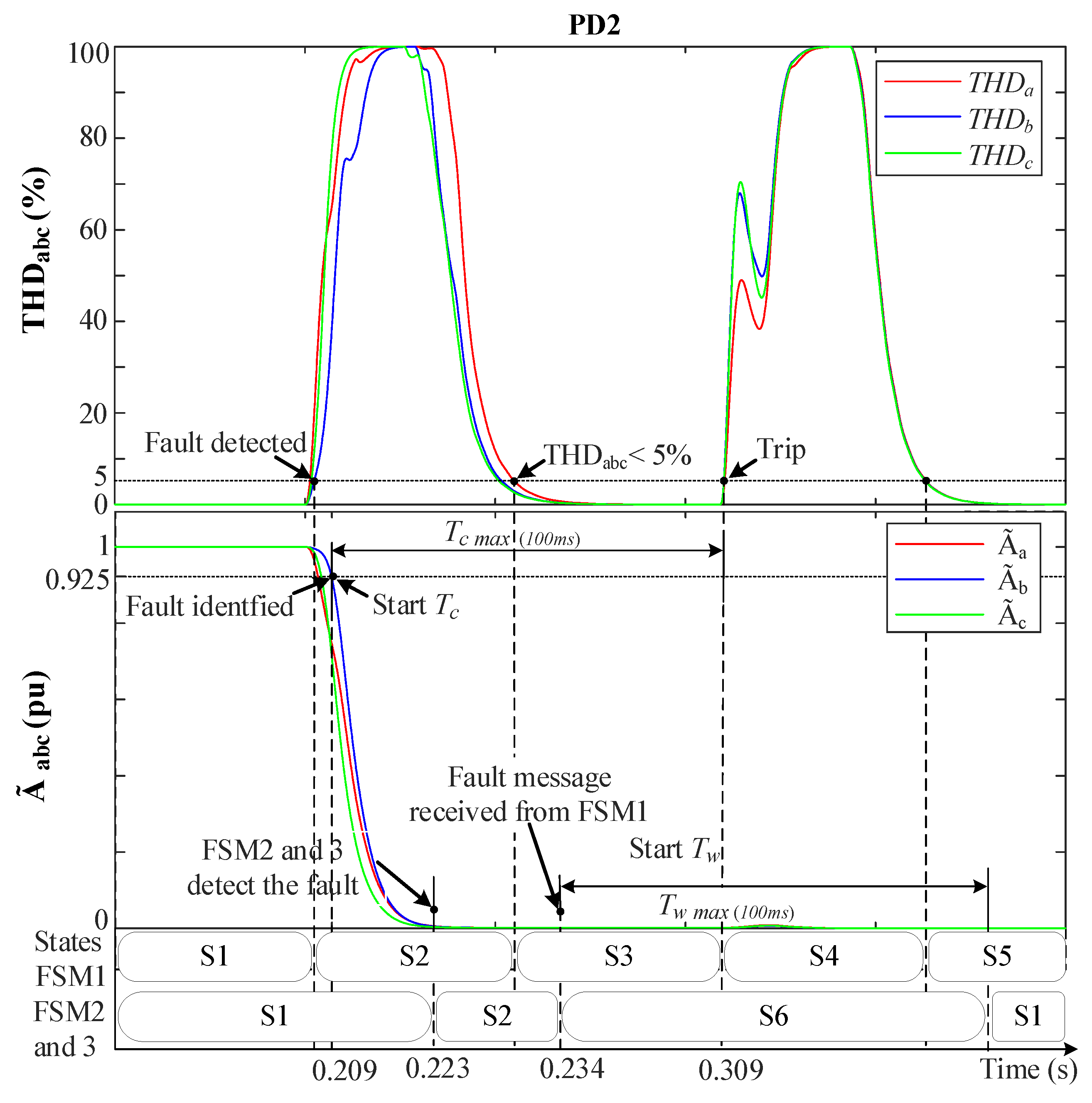
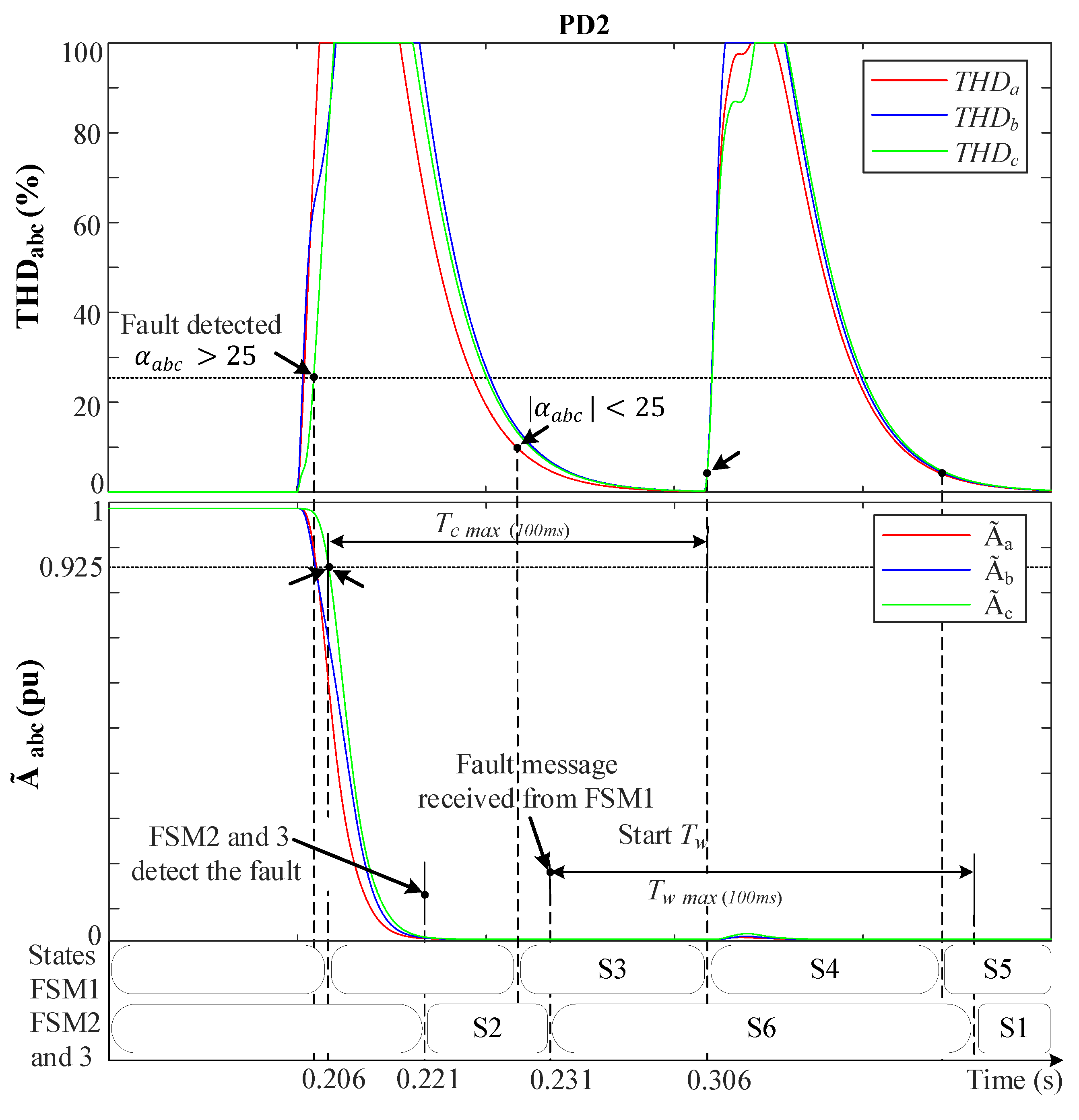
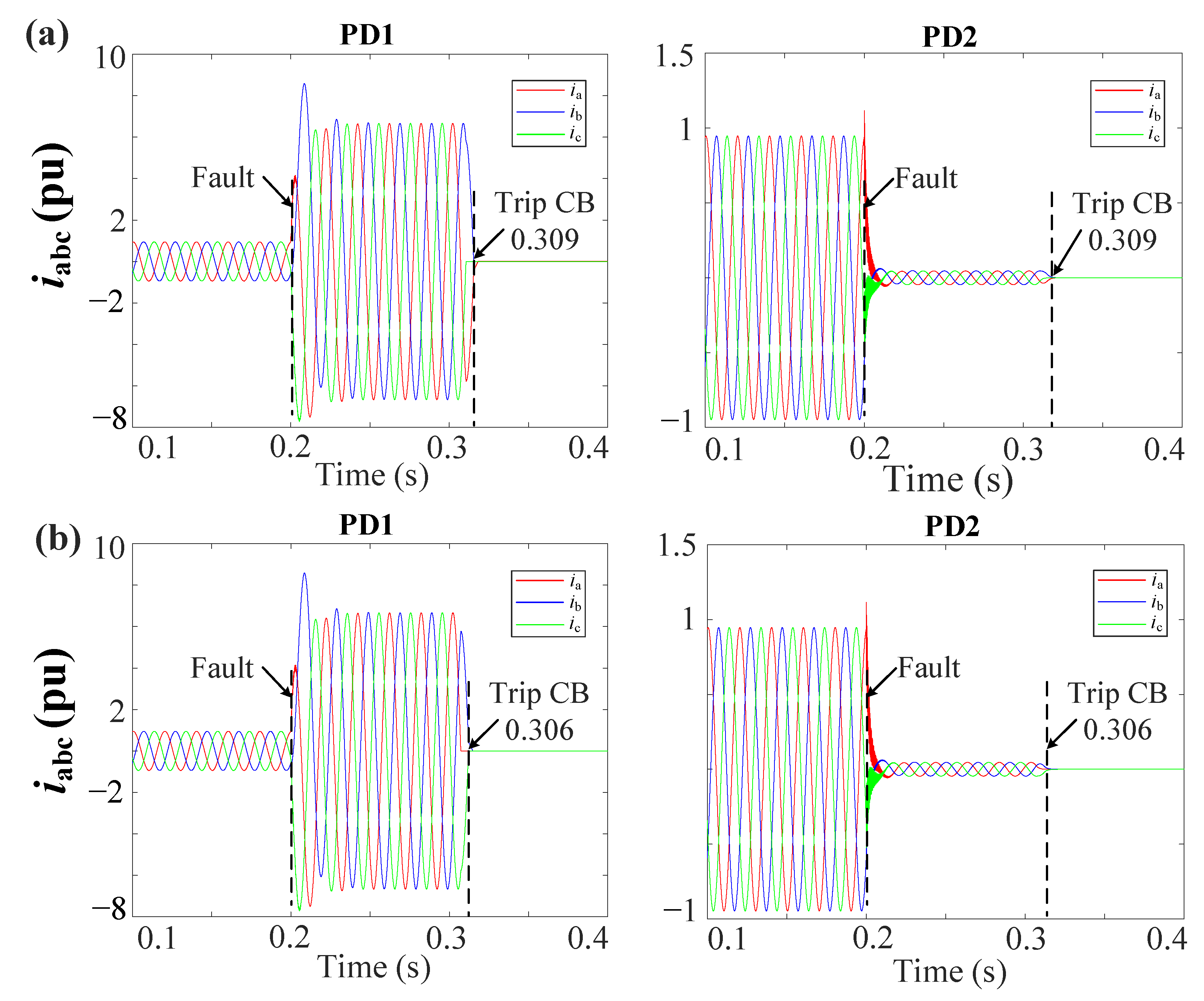
5.1. DG Penetration Protection Test
5.1.1. Three-Phase Fault (3PH-G) at F1
5.1.2. Phase-to-Phase Fault (2PH) at F2
5.2. Comparison with Different Protection Methods
5.2.1. Fault Detection Performance Analysis for the Protection Approaches
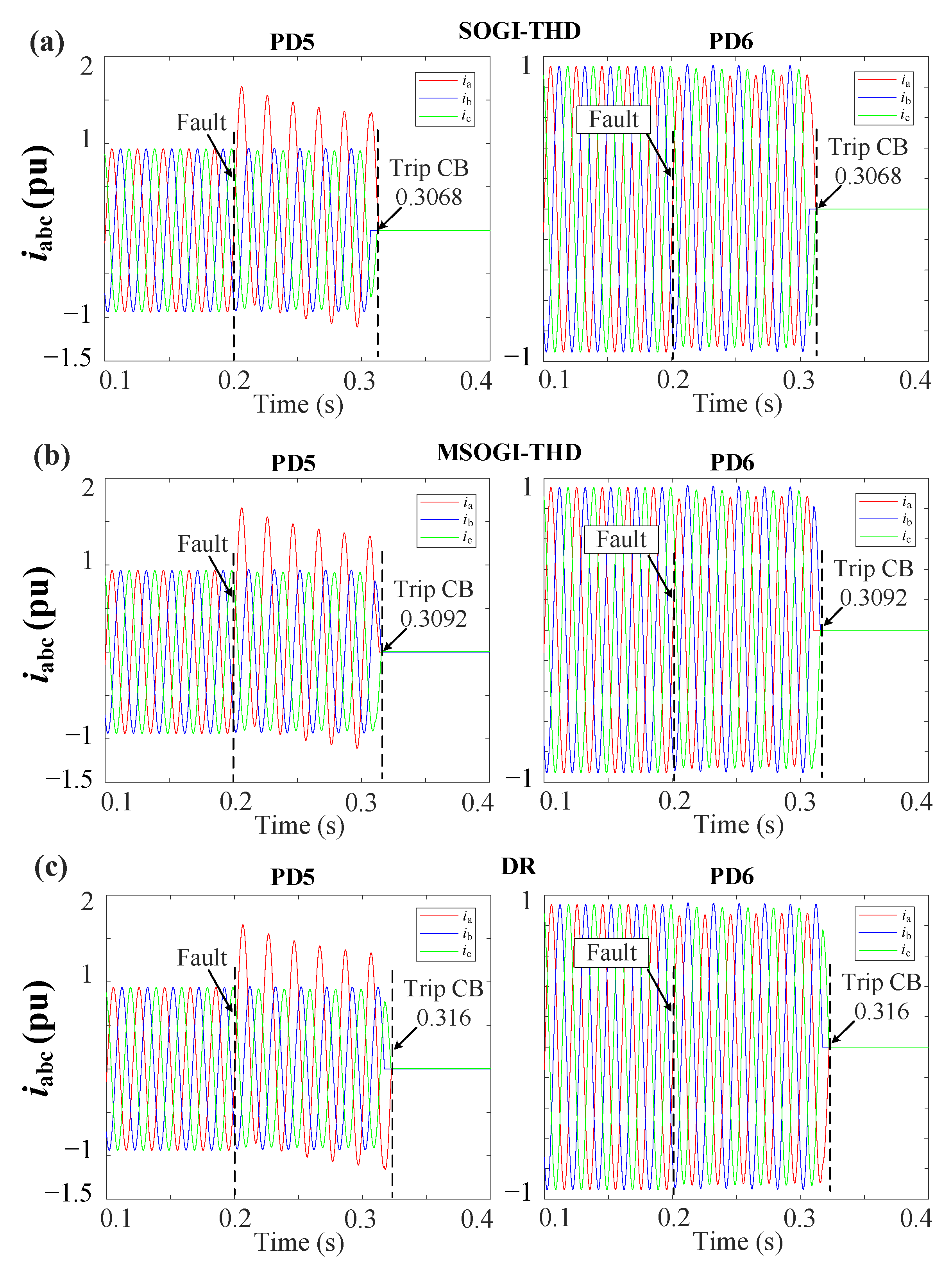
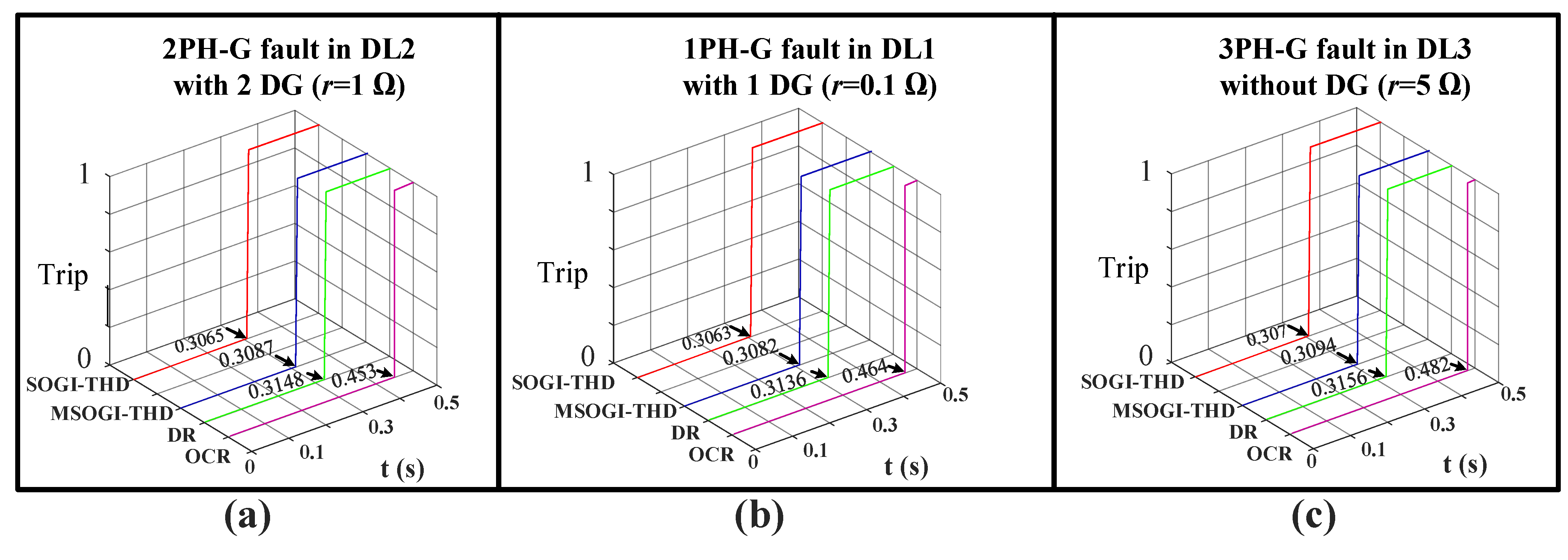
5.2.2. Different Fault Resistance Protection Tests
5.2.3. Different THD Methods Computational Burden Assessment
6. Discussion
7. Conclusions
Author Contributions
Funding
Institutional Review Board Statement
Informed Consent Statement
Data Availability Statement
Conflicts of Interest
References
- Ates, Y.; Uzunoglu, M.; Karakas, A.; Boynuegri, A.R. The Case Study Based Protection Analysis for Smart Distribution Grids Including Distributed Generation Units. In Proceedings of the 12th IET International Conference on Developments in Power System Protection (DPSP 2014), Copenhagen, Denmark, 31 March–3 April 2014; pp. 1–5. [Google Scholar]
- Saadeh, O.S.; Al-Hanaineh, W.; Dalala, Z. Islanding mode operation of a PV supplied network in the presence of G59 protection. In Proceedings of the 2022 IEEE 13th International Symposium on Power Electronics for Distributed Generation Systems (PEDG), Kiel, Germany, 26–29 June 2022; pp. 1–5. [Google Scholar]
- Kennedy, J.; Ciufo, P.; Agalgaonkar, A. A review of protection systems for distribution networks embedded with renewable generation. Renew. Sustain. Energy Rev. 2016, 58, 1308–1317. [Google Scholar] [CrossRef]
- Norshahrani, M.; Mokhlis, H.; Abu Bakar, A.H.; Jamian, J.J.; Sukumar, S. Progress on protection strategies to mitigate the impact of renewable distributed generation on distribution systems. Energies 2017, 10, 1864. [Google Scholar] [CrossRef]
- Meskin, M.; Domijan, A.; Grinberg, I. Impact of distributed generation on the protection systems of distribution networks: Analysis and remedies–review paper. IET Gener. Transm. Distrib. 2020, 14, 5944–5960. [Google Scholar] [CrossRef]
- Bakkar, M.; Bogarra, S.; Córcoles, F.; Iglesias, J.; Al Hanaineh, W. Multi-Layer Smart Fault Protection for Secure Smart Grids. IEEE Trans. Smart Grid 2022, early access. [Google Scholar] [CrossRef]
- Singh, M. Protection coordination in distribution systems with and without distributed energy resources—A review. Prot. Control. Mod. Power Syst. 2017, 2, 27. [Google Scholar] [CrossRef]
- Blaabjerg, F.; Yang, Y.; Yang, D.; Wang, X. Distributed power-generation systems and protection. Proc. IEEE 2017, 105, 1311–1331. [Google Scholar] [CrossRef]
- Senarathna, T.S.S.; Udayanga Hemapala, K.T.M. Review of adaptive protection methods for microgrids. AIMS Energy 2019, 7, 557–578. [Google Scholar] [CrossRef]
- Colson, C.M.; Nehrir, M.H. A review of challenges to real-time power management of microgrids. In Proceedings of the 2009 IEEE Power & Energy Society General Meeting, Calgary, AB, Canada, 26–30 July 2009; pp. 1–8. [Google Scholar]
- Gururajapathy, S.S.; Mokhlis, H.; Illias, H.A. Fault location and detection techniques in power distribution systems with distributed generation: A review. Renew. Sustain. Energy Rev. 2017, 74, 949–958. [Google Scholar] [CrossRef]
- Blackburn, J.L.; Domin, T.J. Protective Relaying Principles and Applications, 4th ed.; Marcel Dekker: New York, NY, USA, 2015. [Google Scholar]
- Beheshtaein, S.; Cuzner, R.; Savaghebi, M.; Guerrero, J.M. Review on microgrids protection. IET Gener. Transm. Distrib. 2019, 13, 743–759. [Google Scholar] [CrossRef]
- Jones, D.; Kumm, J.J. Future Distribution Feeder Protection Using Directional Overcurrent Elements. IEEE Trans. Ind. Appl. 2014, 50, 1385–1390. [Google Scholar] [CrossRef]
- Zeineldin, H.H.; Sharaf, H.M.; Ibrahim, D.K.; El-Zahab, E.E.-D.A. Optimal Protection Coordination for Meshed Distribution Systems with Dg Using Dual Setting Directional Over-Current Relays. IEEE Trans. Smart Grid 2015, 6, 115–123. [Google Scholar] [CrossRef]
- Bakkar, M.; Bogarra, S.; Córcoles, F.; Iglesias, J. Overcurrent protection based on ANNs for smart distribution networks with grid-connected VSIs. IET Gener. Transm. Distrib. 2020, 15, 1159–1174. [Google Scholar] [CrossRef]
- Dewadasa, M.; Ghosh, A.; Ledwich, G. Protection of Microgrids Using Differential Relays. In Proceedings of the Power Engineering Conference (AUPEC), Australasian Universities, Brisbane, Australia, 25–28 September 2011; pp. 1–6. [Google Scholar]
- Ustun, T.S.; Ozansoy, C.; Zayegh, A. Differential Protection of Microgrids with Central Protection Unit Support. In Proceedings of the IEEE 2013 Tencon—Spring, Sydney, Australia, 17–19 April 2013; pp. 15–19. [Google Scholar]
- Hodder, S.; Kasztenny, B.; Fischer, N. Backup considerations for line current differential protection. In Proceedings of the 2012 65th Annual Conference for Protective Relay Engineers, College Station, TX, USA, 2–5 April 2012; pp. 96–107. [Google Scholar]
- Brahma, S.M.; Girgis, A.A. Development of Adaptive Protection Scheme for Distribution Systems with High Penetration of Distributed Generation. IEEE Trans. Power Deliv. 2004, 19, 56–63. [Google Scholar] [CrossRef]
- Ma, J.; Mi, C.; Wang, T.; Wu, J.; Wang, Z. An Adaptive Protection Scheme for Distributed Systems with Distributed Generation. In Proceedings of the Power and Energy Society General Meeting, Detroit, MI, USA, 24–29 July 2011; pp. 1–6. [Google Scholar]
- Choi, J.H.; Nam, S.R.; Nam, H.K.; Kim, J.C. Adaptive protection schemes of Distributed Generation at distribution network for automatic reclosing and voltage sags. In Proceedings of the 2008 IEEE International Conference on Sustainable Energy Technologies, Singapore, 24–27 November 2008; pp. 810–815. [Google Scholar]
- Beheshtaein, S.; Cuzner, R.; Savaghebi, M.; Guerrero, J.M. A new harmonic-based protection structure for meshed microgrids. In Proceedings of the 2018 IEEE Power & Energy Society General Meeting (PESGM), Portland, OR, USA, 5–10 August 2018; pp. 1–6. [Google Scholar]
- Al-Nasseri, H.; Redfern, M.A. Harmonics content based protection scheme for micro-grids dominated by solid state converters. In Proceedings of the 12th International Middle-East Power System Conference, Aswan, Egypt, 12–15 March 2008; pp. 50–56. [Google Scholar]
- Dehghani, M.; Khooban, M.H.; Niknam, T. Fast fault detection and classification based on a combination of wavelet singular entropy theory and fuzzy logic in distribution lines in the presence of distributed generations. Int. J. Electr. Power Energy Syst. 2016, 78, 455–462. [Google Scholar] [CrossRef]
- Ahmadipour, M.; Hizam, H.; Othman, M.L.; Mohd Radzi, M.A.; Chireh, N. A Fast Fault Identification in a Grid-Connected Photovoltaic System Using Wavelet Multi-Resolution Singular Spectrum Entropy and Support Vector Machine. Energies 2019, 12, 2508. [Google Scholar] [CrossRef]
- Pinto, J.O.C.P.; Moreto, M. Protection strategy for fault detection in inverter-dominated low voltage AC microgrid. Electr. Power Syst. Res. 2021, 190, 106572. [Google Scholar] [CrossRef]
- Vyshnavi, G.; Prasad, A. High impedance fault detection using fuzzy logic technique. Int. J. Grid Distrib. Comput. 2018, 11, 13–22. [Google Scholar] [CrossRef]
- Gush, T.; Bukhari, S.B.A.; Haider, R.; Admasie, S.; Oh, Y.S.; Cho, G.J.; Kim, C.H. Fault detection and location in a microgrid using mathematical morphology and recursive least square methods. Int. J. Electr. Power Energy Syst. 2018, 102, 324–331. [Google Scholar] [CrossRef]
- Manohar, M.; Koley, E.; Ghosh, S. Microgrid protection against high impedance faults with robustness to harmonic intrusion and weather intermittency. IET Renew. Power Gener. 2021, 15, 2325–2339. [Google Scholar] [CrossRef]
- Sharma, N.K.; Samantaray, S.R. Validation of differential phaseangle based microgrid protection scheme on RTDS platform. In Proceedings of the 20th National Power Systems Conference (NPSC), Tiruchirappalli, India, 14–16 December 2018; pp. 1–6. [Google Scholar] [CrossRef]
- Eslami, R.; Sadeghi, S.H.H.; Abyaneh, H.A. A probabilistic approach for the evaluation of fault detection schemes in microgrids. Eng. Technol. Appl. Sci. Res. 2017, 7, 1967–1973. [Google Scholar] [CrossRef]
- Roy, S.; Debnath, S. PSD based high impedance fault detection and classification in distribution system. Measurement 2021, 169, 108366. [Google Scholar] [CrossRef]
- Gashteroodkhani, O.A.; Majidi, M.; Etezadi-Amoli, M. A combined deep belief network and time-time transform based intelligent protection Scheme for microgrids. Electr. Power Syst. Res. 2020, 182, 106239. [Google Scholar] [CrossRef]
- Mishra, M.; Rout, P.K. Detection and classification of micro-grid faults based on HHT and machine learning techniques. IET Gener. Transm. Distrib. 2018, 12, 388–397. [Google Scholar] [CrossRef]
- Al Hanaineh, W.; Matas, J.; El Mariachet, J.; Xie, P.; Bakkar, M.; Guerrero, J.M. A THD-Based Fault Protection Method Using MSOGI-FLL Grid Voltage Estimator. Sensors 2023, 23, 980. [Google Scholar] [CrossRef] [PubMed]
- Al Hanaineh, W.; Matas, J.; Bakkar, M.; Guerrero, J.M. A Robust THD Based Communication-Less Protection Method for Electrical Grids with DGs. 2023. manuscript under review. [Google Scholar]
- Santoso, S.; McGranaghan, M.F.; Dugan, R.C.; Beaty, H.W. Electrical Power Systems Quality, 3rd ed.; McGraw-Hill Education: New York, NY, USA, 2012. [Google Scholar]
- Kusko, A. Power Quality in Electrical Systems; McGraw-Hill Education: New York, NY, USA, 2007. [Google Scholar]
- Rodríguez, P.; Luna, A.; Candela, I.; Mujal, R.; Teodorescu, R.; Blaabjerg, F. Multiresonant frequency-locked loop for grid synchronization of power converters under distorted grid conditions. IEEE Trans. Ind. Electron. 2010, 58, 127–138. [Google Scholar] [CrossRef]
- Yazdani, A.; Iravani, R. Voltage-Sourced Converters in Power Systems: Modeling, Control, and Applications; John Wiley & Sons: Toronto, ON, Canada, 2010. [Google Scholar]
- Al Hanaineh, W.; Matas, J.; El Mariachet, J.; Guerrero, J.M. A Harmonic-based Fault detection algorithm for Microgrids. In Proceedings of the Interdisciplinary Conference on Mechanics, Computers and Electrics (ICMECE 2022), Barcelona, Spain, 6–7 October 2022. [Google Scholar]
- Matas, J.; Martín, H.; de la Hoz, J.; Abusorrah, A.; Al-Turki, Y.; Alshaeikh, H. A new THD measurement method with small computational burden using a SOGI-FLL grid monitoring system. IEEE Trans. Power Electron. 2019, 35, 5797–5811. [Google Scholar] [CrossRef]
- NTP-CT: Technical Conditions and Safety of EDNESA Distribution Installations; Endesa: Madrid, Spain, 2007; p. 4827.
- IEEE Std 519-2014 (Revision of IEEE Std 519-1992); IEEE Recommended Practice and Requirements for Harmonic Control in Electric Power Systems. IEEE: New York, NY, USA, 2014; pp. 1–29. [CrossRef]
- P.O.12.2: Technical Requirements of Wind Power and Photovoltaic Facilities (Draft); Red Electra: Madrid, Spain, 2008.
- Bollen, M.H. Understanding power quality problems. In Voltage Sags and Interruptions; IEEE Press: Piscataway, NJ, USA, 2000. [Google Scholar]
- Hong, P.; Turk, M.; Huang, T.S. Gesture modeling and recognition using finite state machines. In Proceedings of the Fourth IEEE International Conference on Automatic Face and Gesture Recognition (Cat. No. PR00580), Grenoble, France, 28–30 March 2000; pp. 410–415. [Google Scholar]
- Silos, Á.; Señís, A.; Martín de Pozuelo, R.; Zaballos, A. Using IEC 61850 goose service for adaptive ANSI 67/67N protection in ring main systems with distributed energy resources. Energies 2017, 10, 1685. [Google Scholar] [CrossRef]
- Ustun, T.S.; Ozansoy, C.; Zayegh, A. Modeling of a centralized microgrid protection system and distributed energy resources according to IEC 61850-7-420. IEEE Trans. Power Syst. 2012, 27, 1560–1567. [Google Scholar] [CrossRef]
- Shabani, A.; Mazlumi, K. Evaluation of a communication-assisted overcurrent protection scheme for photovoltaic-based DC microgrid. IEEE Trans. Smart Grid 2019, 11, 429–439. [Google Scholar] [CrossRef]
- IEC61850; IEC Communications Networks and Systems in Substations. ABB Co.: Vasteras, Sweden, 2011. Available online: https://www.google.com/url?sa=t&rct=j&q=&esrc=s&source=web&cd=&ved=2ahUKEwi4u8Slhfr-AhW2gP0HHfh8BZcQFnoECAwQAQ&url=https%3A%2F%2Fwww.gegridsolutions.com%2Fmultilin%2Fjournals%2Fisues%2Fspring09%2Fiec61850.pdf&usg=AOvVaw2SBaCDgCisHQrtd9VF2F-i (accessed on 13 March 2023).
- Kezunovic, M.; Ren, J.; Lotfifard, S. Design, Modeling and Evaluation of Protective Relays for Power Systems; Springer International Publishing: Cham, Switzerland, 2016. [Google Scholar]
- Bakkar, M.; Bogarra, S.; Córcoles, F.; Aboelhassan, A.; Wang, S.; Iglesias, J. Artificial Intelligence-Based Protection for Smart Grids. Energies 2022, 15, 4933. [Google Scholar] [CrossRef]
- van der Walt, H.L.; Bansal, R.C.; Naidoo, R. PV based distributed generation power system protection: A review. Renew. Energy Focus 2018, 24, 33–40. [Google Scholar] [CrossRef]
- Mirsaeidi, S.; Said, D.M.; Mustafa, M.W.; Habibuddin, M.H.; Ghaffari, K. An analytical literature review of the available techniques for the protection of micro-grids. Int. J. Electr. Power Energy Syst. 2014, 58, 300–306. [Google Scholar] [CrossRef]
- Baran, M.E.; Hooshyar, H.; Shen, Z.; Huang, A. Accommodating high PV penetration on distribution feeders. IEEE Trans. Smart Grid 2012, 3, 1039–1046. [Google Scholar] [CrossRef]
- Benmouyal, G.; Meisinger, M.; Burnworth, J.; Elmore, W.A.; Freirich, K.; Kotos, P.A.; Leblanc, P.R.; Lerley, P.J.; McConnell, J.E.; Mizener, J.; et al. IEEE standard inverse-time characteristic equations for overcurrent relays. IEEE Trans. Power Deliv. 1999, 14, 868–871. [Google Scholar] [CrossRef]
- Shih, M.Y.; Conde, A.; Leonowicz, Z.; Martirano, L. An adaptive overcurrent coordination scheme to improve relay sensitivity and overcome drawbacks due to distributed generation in smart grids. IEEE Trans. Ind. Appl. 2017, 53, 5217–5228. [Google Scholar] [CrossRef]
- Hong, L.; Rizwan, M.; Wasif, M.; Ahmad, S.; Zaindin, M.; Firdausi, M. User-Defined Dual Setting Directional Overcurrent Relays with Hybrid Time Current-Voltage Characteristics-Based Protection Coordination for Active Distribution Network. IEEE Access 2021, 9, 62752–62769. [Google Scholar] [CrossRef]
- Sharaf, H.M.; Zeineldin, H.H.; El-Saadany, E. Protection coordination for microgrids with grid-connected and islanded capabilities using communication assisted dual setting directional overcurrent relays. IEEE Trans. Smart Grid 2018, 9, 143–151. [Google Scholar] [CrossRef]
- Shih, M.Y.; Conde, A.; Ángeles-Camacho, C.; Fernández, E.; Leonowicz, Z.; Lezama, F.; Chan, J. A two stage fault current limiter and directional overcurrent relay optimization for adaptive protection resetting using differential evolution multi-objective algorithm in presence of distributed generation. Electr. Power Syst. Res. 2021, 190, 106844. [Google Scholar] [CrossRef]
- He, J.; Liu, L.; Xu, Y.; Ding, F.; Zhang, D. A two-step protection algorithm for smart distribution systems with DGs. Int. Trans. Electr. Energy Syst. 2018, 28, e2506. [Google Scholar] [CrossRef]
- Manohar, M.; Koley, E.; Ghosh, S. Enhancing the reliability of protection scheme for PV integrated microgrid by discriminating between array faults and symmetrical line faults using sparse auto encoder. IET Renew. Power Gener. 2019, 13, 308–317. [Google Scholar] [CrossRef]


| Main Grid | HV/MV Transformer (YNd11) | Distribution Lines (DLs) | MV/LV Transformer (Dyn11) | DGs Rating |
|---|---|---|---|---|
| Rated voltage: 66 kV Short circuit power: 360 MVA | Rated power: 20 MVA Rated Voltage: 66/20 kV Usc (%): 11 | Resistance: 0.16 Ω/km Reactance: 0.109 H/km Capacitance: 0.31 μF/km Length of line: 2 km | Rated power: 400 kVA Rated Voltage: 20/0.4 kV Usc (%): 4.5 | Rated power: 6 MVA Rated Voltage: 400 V |
| Fault Type | Location | Defined as | Contribution of DG | Extra Communication Delay | Harmonics Previous to the Fault | |
|---|---|---|---|---|---|---|
| 3PH-G | DL1 | F1 | DG1 = 6 MW DG2 = 6 MW | 25 ms | No | Zero |
| 2PH | DL3 | F2 | DG1 = Zero DG2 = Zero | Zero | Yes | 5% of 5th Harmonic |
| Parameter | Value |
|---|---|
| Pick up current (pu) | 1 |
| Time dial (TD) | 0.5 |
| Current transformer ratio (CT) | 500:1 |
| Parameter | Value |
|---|---|
| Differential current (pu) | 1.08 |
| Biased characteristic (K) | 0.5 |
| Current transformer ratio (CT) | 500:1 |
| Approach | Fault Detection Time (ms) | Fault Clearing Time (s) |
|---|---|---|
| SOGI-THD | 6.0 | 0.3060 |
| MSOGI-THD | 9.0 | 0.3090 |
| DR | 15.0 | 0.3150 |
| OCR | 175.0 | 0.4750 |
| Method | Number of SOGIs | Number of Cycles (c) |
|---|---|---|
| SOGI-THD | 3 | 447 |
| MSOGI-THD | 12 | 1788 |
| FFT-THD | Not applicable | 21,057 |
| References | Protection Strategies | Parameter Used | Speed | Accuracy | Cost | Inverter Based | Communication | Grid Configuration |
|---|---|---|---|---|---|---|---|---|
| [25] | Wavelet individual entropy and fuzzy inference system | Current | High | High | Low | Yes | Not Required | Radial |
| [28] | fuzzy logic technique | Current | High | Medium | Low | No | Not Required | Radial/Ring |
| [26] | Wavelet transform and support vector mechanism | Voltage | Medium | High | High | No | Not Required | Radial/Ring |
| [29] | Statistical morphology, recursive least square methods and Butterworth filter | Current | High | High | High | Yes | Required | Ring |
| [31] | Differential phase angle criteria | Voltage | High | High | High | Yes | Required | Ring |
| [32] | S-transform | Current and Voltage | Medium | Medium | High | Yes | Required | Radial |
| [33] | Power spectral density and transform. | Current | High | High | High | Yes | Not Required | Radial |
| [34] | Deep belief network, time-time transform and PUM | Current | Low | High | High | Yes | Required | Radial/Ring |
| [27] | Traveling wave and wavelet analysis | Current | High | High | High | No | Required | Radial |
| [30] | Least square Adaline algorithm and modified support vector mechanism | Current | Medium | High | High | Yes | Not Required | Radial/Ring |
| [35] | Hilbert-Huang Transform differential relay | Current | High | High | High | Yes | Required | Ring |
| [37] | SOGI-THD | Voltage | High | High | Low | Yes | Required | Radial |
| References | Protection Strategies | Trip Time | Advantages | Disadvantages |
|---|---|---|---|---|
| [59] | Centralize Controller and Linear Programming | 421 ms | Relay settings can be obtained instantly without requiring any training | Possibility of communication failures, the complexity grows with a higher number of buses |
| [60] | Multi-Agent System and OCR | 300 ms | No central controller | Possibility of communication failures |
| [61] | OCR | >200 ms | Variable fault resistance and DG penetration | Not adaptable for network modifications |
| [62] | Dual settings OCR | >100 ms | Variable fault resistance and DG penetration | Offline calculation |
| [63] | Multi-Terminal DR | 90 ms | Fast, variable fault resistance and DG penetration | Possibility of communication failures |
| [23] | THD | 20–50 ms | Fast, no need for a voltage transformer | Possibility of communication failures, validated only for three-phase faults |
| [64] | Deep neural network | 20–30 | Fast, variable fault resistance and DG penetration | Possibility of communication failures and inflexibility in the case of network modifications |
| [16] | OC and ANN | 14 ms | Fast, variable fault resistance and DG penetration | Possibility of communication failures, a complex training process, and inflexibility in the case of network modifications |
| [36] | MSOGI-THD | 7–10 ms | Fast tripping, variable fault location and types, variable fault resistance and DG penetration, affordable computational burden. | Possibility of communication failures |
| [37] | SOGI-THD | 6–8.5 ms | The same merits of the MSOGI-THD. In addition, it is faster and more reliable with a higher THD threshold, requires fewer SOGIs, and has a lower computational burden. | Possibility of communication failures. |
Disclaimer/Publisher’s Note: The statements, opinions and data contained in all publications are solely those of the individual author(s) and contributor(s) and not of MDPI and/or the editor(s). MDPI and/or the editor(s) disclaim responsibility for any injury to people or property resulting from any ideas, methods, instructions or products referred to in the content. |
© 2023 by the authors. Licensee MDPI, Basel, Switzerland. This article is an open access article distributed under the terms and conditions of the Creative Commons Attribution (CC BY) license (https://creativecommons.org/licenses/by/4.0/).
Share and Cite
Al Hanaineh, W.; Matas, J.; Guerrero, J.M. A Comparative Study of Smart THD-Based Fault Protection Techniques for Distribution Networks. Sensors 2023, 23, 4874. https://doi.org/10.3390/s23104874
Al Hanaineh W, Matas J, Guerrero JM. A Comparative Study of Smart THD-Based Fault Protection Techniques for Distribution Networks. Sensors. 2023; 23(10):4874. https://doi.org/10.3390/s23104874
Chicago/Turabian StyleAl Hanaineh, Wael, Jose Matas, and Josep M. Guerrero. 2023. "A Comparative Study of Smart THD-Based Fault Protection Techniques for Distribution Networks" Sensors 23, no. 10: 4874. https://doi.org/10.3390/s23104874