

Current Sensorless Based on PI MPPT Algorithms
 ,
,  , and
, and
Abstract
:1. Introduction
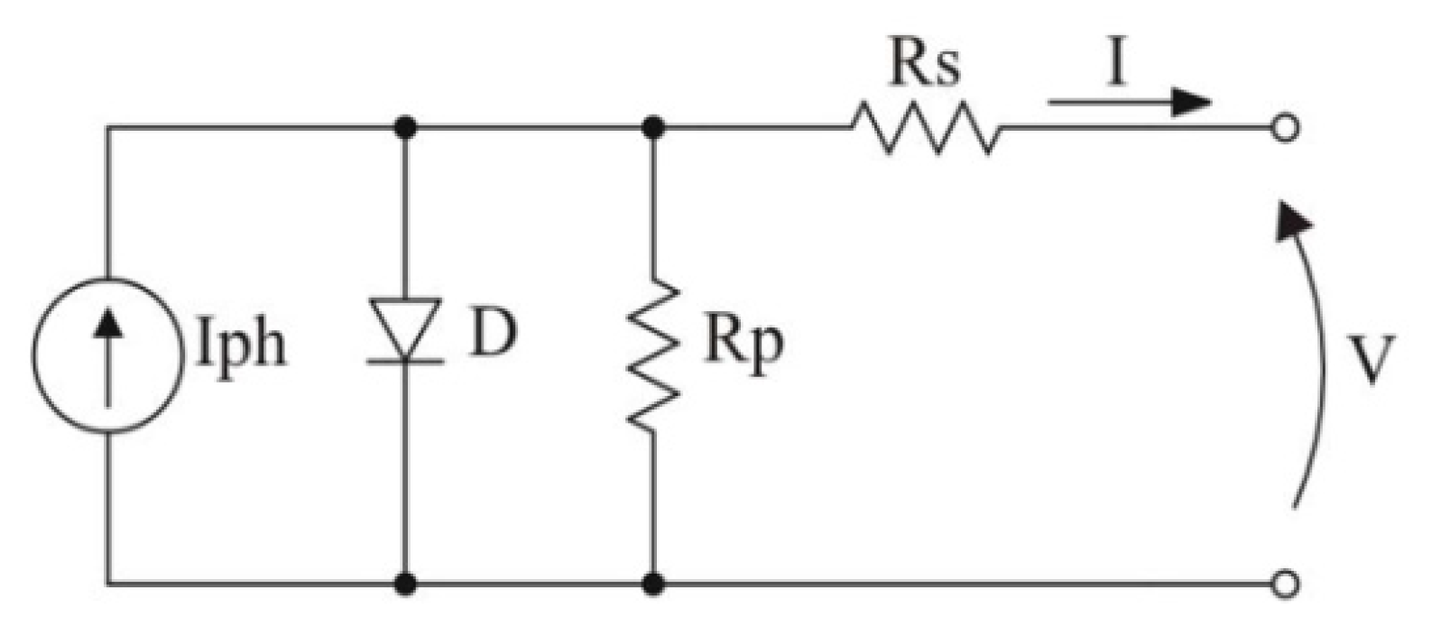
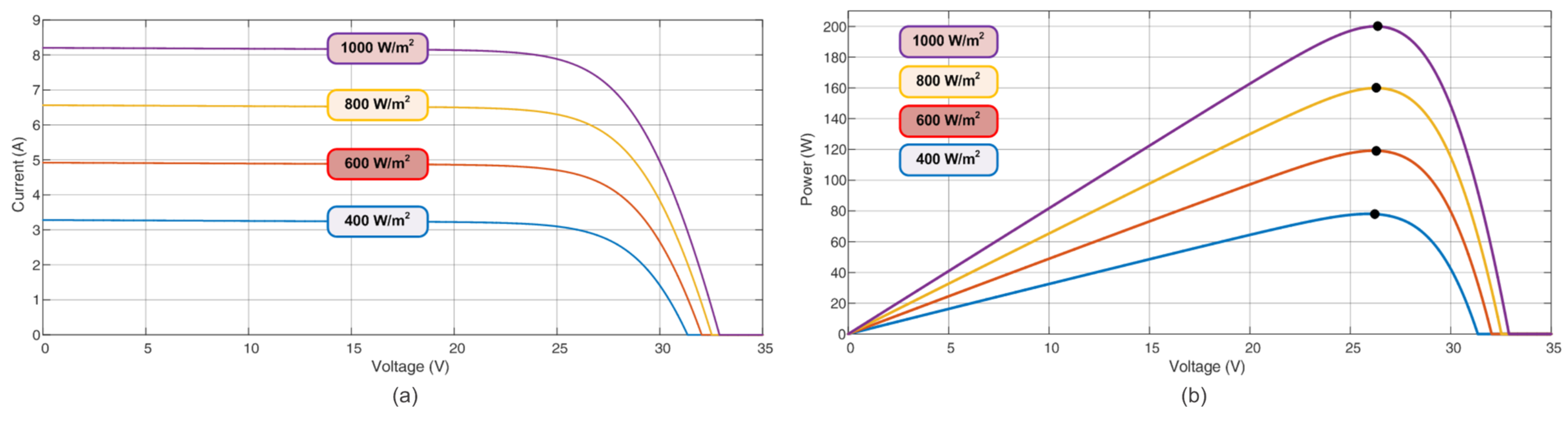
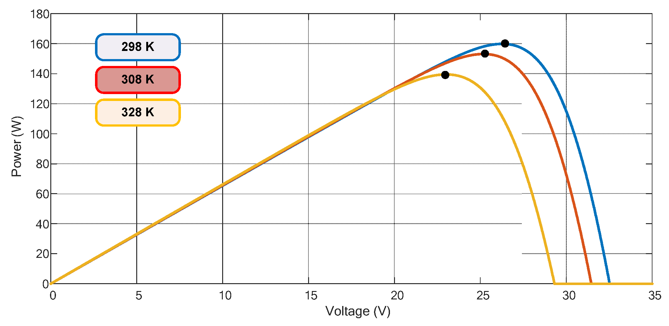
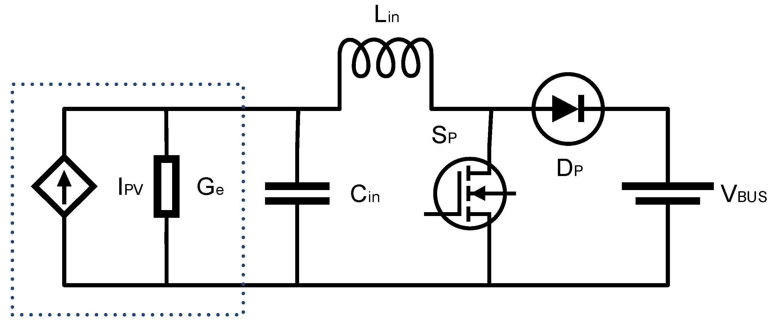
2. PV Modeling
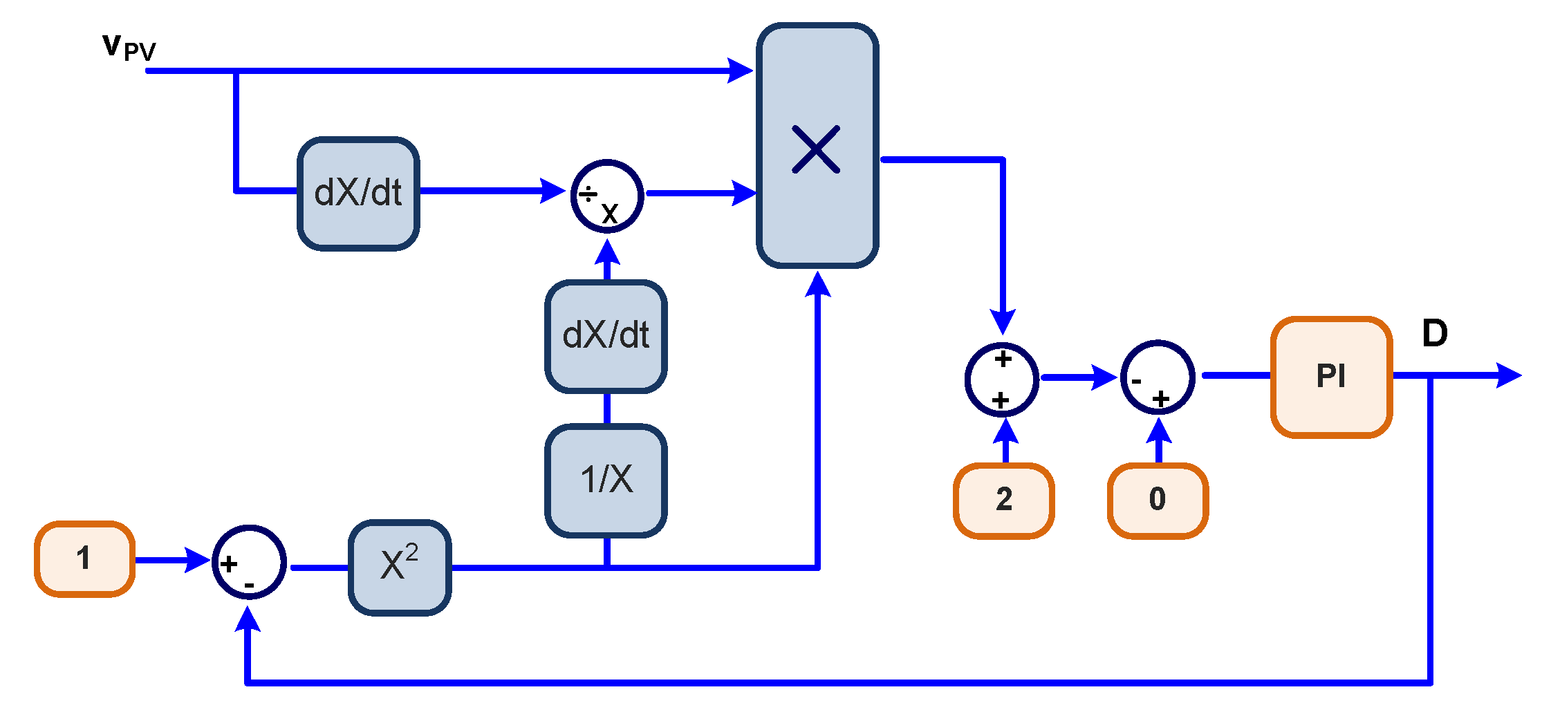
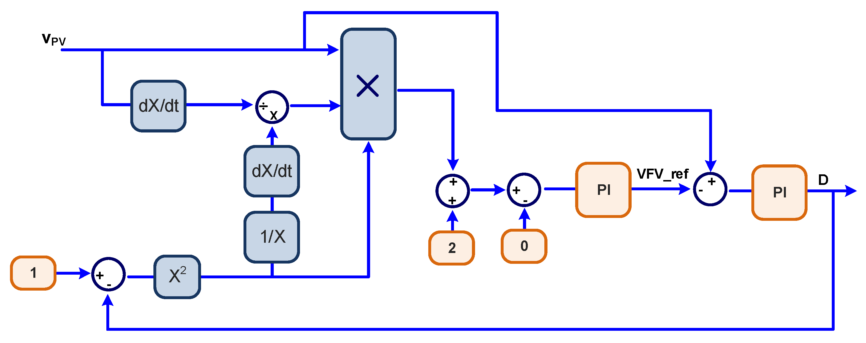
3. Proposed MPPT Mathematical Modeling
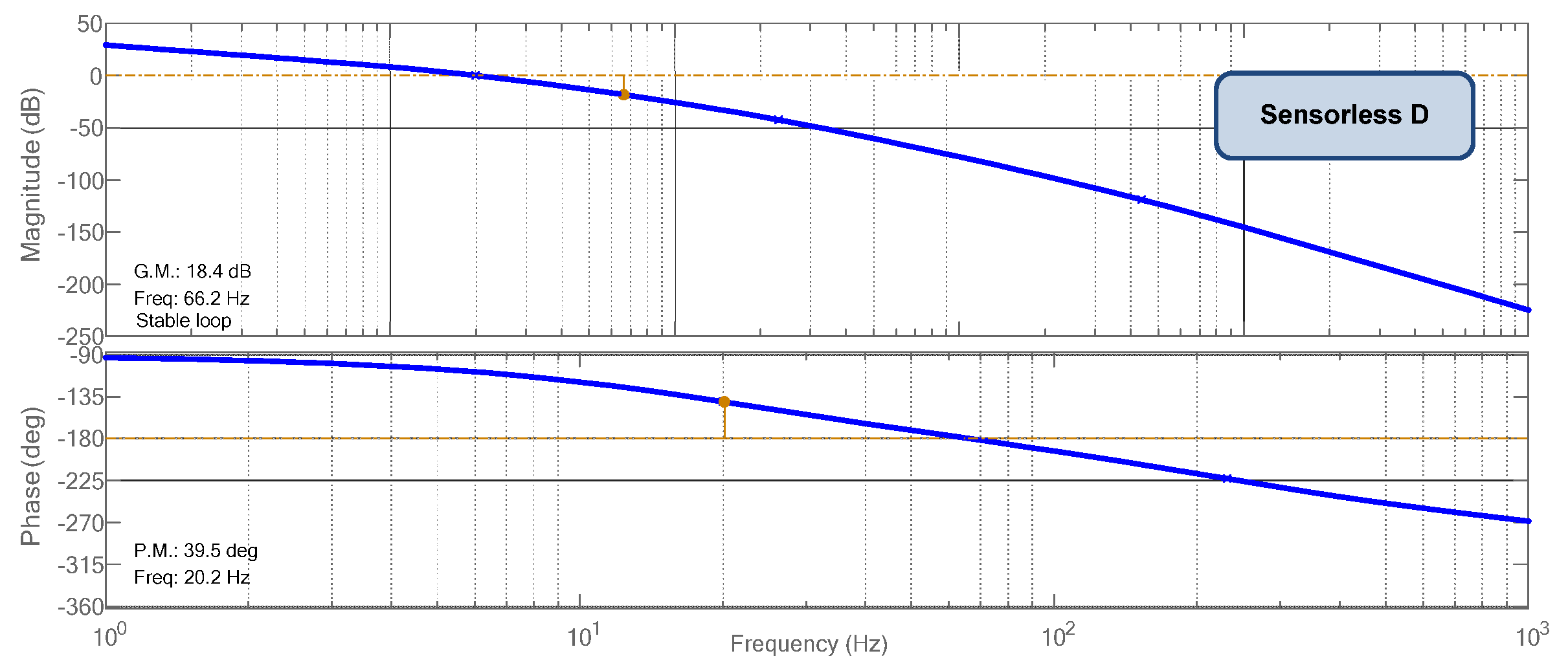
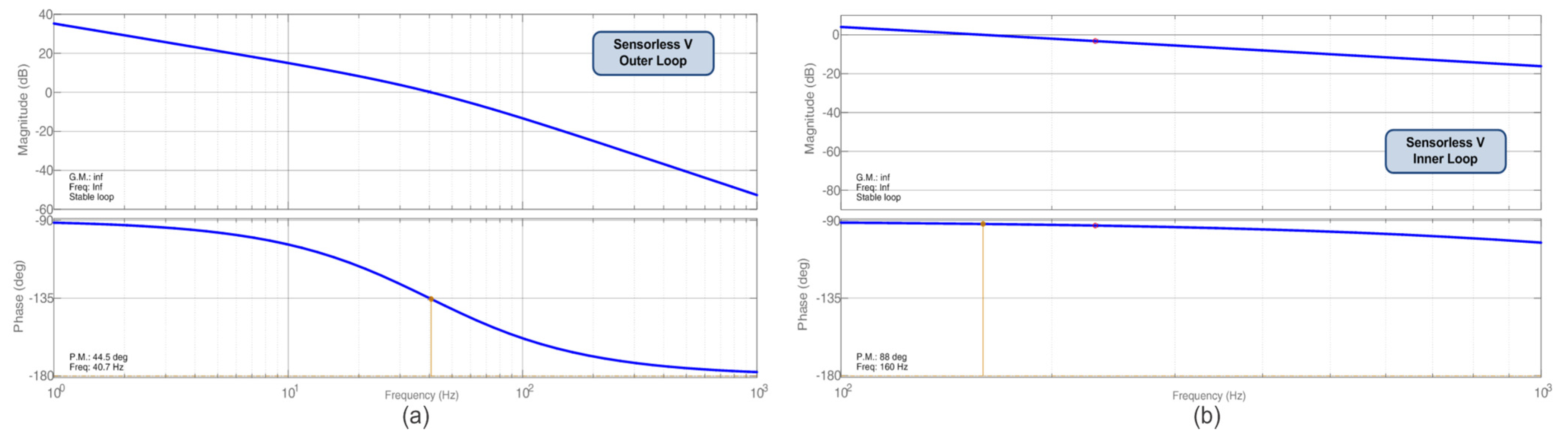
4. Controlled MPPT Transfer Functions
5. Results and Discussion
6. Perovskite Solar Cells
7. Conclusions
Author Contributions
Funding
Institutional Review Board Statement
Informed Consent Statement
Data Availability Statement
Acknowledgments
Conflicts of Interest
References
- Liserre, E.M.; Sauter, T.; Hung, J.Y. Future Energy Systems: Integrating Renewable Energy Sources into the Smart Power Grid Through Industrial Electronics. IEEE Ind. Electron. Mag. 2010, 4, 18–37. [Google Scholar] [CrossRef]
- Kwon, J.; Nam, K.; Kwon, B. Photovoltaic Power Conditioning System with Line Connection. IEEE Trans. Ind. Electron. 2006, 53, 1048–1054. [Google Scholar] [CrossRef]
- IRENA—International Renewable Energy Agency. Trends in Renewable Energy: Statistic Time SeRies. 2021. Available online: https://www.irena.org/Statistics/View-Data-by-Topic/Capacity-and-Generation/Statistics-Time-Series (accessed on 10 December 2022).
- Philipps, S.; Warmuth, W. Fraunhofer Institute for Solar energy systems. In Photovoltaics Report; Freiburg, Germany, 2019; pp. 1–49. [Google Scholar]
- NREL—National Renewable Energy Laboratory. Photovoltaic Research: Best Research-Cell Efficiency Chart. 2019. Available online: https://www.nrel.gov/pv/cell-efficiency.html (accessed on 10 December 2022).
- Ahmed, S.; Mekhilef, S.; Mubin, M.B.; Tey, K.S. Performances of the adaptive conventional maximum power point tracking algorithms for solar photovoltaic system. Sustain. Energy Technol. Assessments 2022, 53, 102390. [Google Scholar] [CrossRef]
- de Brito, M.A.G.; Galotto, L.; Sampaio, L.P.; Melo, G.D.A.E.; Canesin, C.A. Evaluation of the Main MPPT Techniques for Pho-tovoltaic Applications. IEEE Trans. Ind. Electron. 2013, 60, 1156–1167. [Google Scholar] [CrossRef]
- Sarvi, M.; Azadian, A. A comprehensive review and classified comparison of MPPT algorithms in PV systems. Energy Syst. 2021, 13, 281–320. [Google Scholar] [CrossRef]
- Erickson, R.; Maksimovic, D.M. Fundamentals of Power Electronics, 2nd ed.; Kluwer Academic: Secaucus, NJ, USA, 2017; p. 882. [Google Scholar]
- Femia, N.; Petrone, G.; Spagnuolo, G.; Vitelli, M. Optimization of Perturb and Observe Maximum Power Point Tracking Method. IEEE Trans. Power Electron. 2005, 20, 963–973. [Google Scholar] [CrossRef]
- Abdelsalam, A.K.; Massoud, A.M.; Ahmed, S.; Enjeti, P.N. High-Performance Adaptive Perturb and Observe MPPT Technique for Photovoltaic-Based Microgrids. IEEE Trans. Power Electron. 2011, 26, 1010–1021. [Google Scholar] [CrossRef]
- Yu, W.L.; Lee, T.-P.; Wu, G.-H.; Chen, Q.S.; Chiu, H.-J.; Lo, Y.-K.; Shih, F. A DSP-based single-stage maximum power point tracking PV inverter. In Proceedings of the Twenty-Fifth Annual IEEE Applied Power Electronics Conference and Exposition (APEC), Palm Springs, CA, USA, 21–25 February 2010; Volume 25, pp. 948–952. [Google Scholar]
- Gunasekaran, M.; Krishnasamy, V.; Selvam, S.; Almakhles, D.J.; Anglani, N. An Adaptive Resistance Perturbation Based MPPT Algorithm for Photovoltaic Applications. IEEE Access 2020, 8, 196890–196901. [Google Scholar] [CrossRef]
- Hsieh, G.-C.; Chen, H.-L.; Chen, Y.; Tsai, C.-M.; Shyu, S.-S. Variable frequency controlled incremental conductance derived MPPT photovoltaic stand-along DC bus system. In Proceedings of the 2008 Twenty-Third Annual IEEE Applied Power Electronics Conference and Exposition, Austin, TX, USA, 24–28 February 2008; Volume 23, pp. 1849–1854. [Google Scholar]
- Liu, F.; Duan, S.; Liu, F.; Liu, B.; Kang, Y. A Variable Step Size INC MPPT Method for PV Systems. IEEE Trans. Ind. Electron. 2008, 55, 2622–2628. [Google Scholar]
- Tey, K.S.; Mekhilef, S. Modified Incremental Conductance Algorithm for Photovoltaic System Under Partial Shading Conditions and Load Variation. IEEE Trans. Ind. Electron. 2014, 61, 5384–5392. [Google Scholar]
- Alsumiri, M. Residual Incremental Conductance Based Nonparametric MPPT Control for Solar Photovoltaic Energy Control for Solar Photovoltaic Energy Conversion System. IEEE Access 2019, 7, 87901–87906. [Google Scholar] [CrossRef]
- Jain, S.; Agarwal, V. A New Algorithm for Rapid Tracking of Approximate Maximum Power Point in Photovoltaic Systems. IEEE Power Electron. Lett. 2004, 2, 16–19. [Google Scholar] [CrossRef]
- Casadei, D.; Grandi, G.; Rossi, C. Single-Phase Single-Stage Photovoltaic Generation System Based on a Ripple Correlation Control Maximum Power Point Tracking. IEEE Trans. Energy Convers. 2006, 21, 562–568. [Google Scholar] [CrossRef]
- Esram, T.; Kimball, J.; Krein, P.; Chapman, P.; Midya, P. Dynamic maximum power point tracking of photovoltaic arrays using ripple correlation control. IEEE Trans. Power Electron. 2006, 21, 1282–1291. [Google Scholar] [CrossRef]
- Ho, B.M.T.; Chung, H.S.H.; Lo, W.L. Use of System Oscillation to Locate the MPP of PV Panels. IEEE Power Electron. Lett. 2004, 2, 1–5. [Google Scholar] [CrossRef]
- Ho, B.; Chung, H.; Hui, S. An integrated inverter with maximum power tracking for grid-connected PV systems. IEEE Trans. Power Electron. 2005, 20, 953–962. [Google Scholar] [CrossRef]
- Scarpa, V.V.R.; Buzo, S.; Spiazzi, G. Low complexity MPPT technique exploiting the effect of the PV Module MPP Locus char-acterization. IEEE Trans. Ind. Electron. 2009, 56, 1531–1538. [Google Scholar] [CrossRef]
- Singh, Y.; Pal, N. Reinforcement learning with fuzzified reward approach for MPPT control of PV systems. Sustain. Energy Technol. Assessments 2021, 48, 101665. [Google Scholar] [CrossRef]
- Inthamoussou, F.A.; Valenciaga, F. A fast and robust closed-loop photovoltaic MPPT approach based on sliding mode techniques. Sustain. Energy Technol. Assessments 2021, 47, 101665. [Google Scholar] [CrossRef]
- de Brito, M.A.G.; Prado, V.A.; Batista, E.A.; Alves, M.G.; Canesin, C.A. Design Procedure to Convert a Maximum Power Point Tracking Algorithm into a Loop Control System. Energies 2021, 14, 4550. [Google Scholar] [CrossRef]
- Killi, M.; Samanta, S. An Adaptive Voltage-Sensor-Based MPPT for Photovoltaic Systems with SEPIC Converter Including Steady-State and Drift Analysis. IEEE Trans. Ind. Electron. 2015, 62, 7609–7619. [Google Scholar] [CrossRef]
- Dallago, E.; Finarelli, D.G.; Gianazza, U.P.; Barnabei, A.L.; Liberale, A. Theoretical and Experimental Analysis of an MPP Detection Algorithm Employing a Single-Voltage Sensor Only and a Noisy Signal. IEEE Trans. Power Electron. 2013, 28, 5088–5097. [Google Scholar] [CrossRef]
- Hua, C.C.; Fang, Y.H.; Chen, W.T. Hybrid maximum power point tracking method with variable step size for photovoltaic systems. IET Renew. Power Gener. 2016, 10, 127–132. [Google Scholar] [CrossRef]
- Pandey, A.; Dasgupta, N.; Mukerjee, A.K. A Simple Single-Sensor MPPT Solution. IEEE Trans. Power Electron. 2007, 22, 698–700. [Google Scholar] [CrossRef]
- Seo, G.S.; Shin, J.W.; Cho, B.H.; Lee, K.C. Digitally controlled current sensorless photovoltaic micro-converter for dc distri-bution. IEEE Trans. Ind. Inform. 2014, 10, 117–126. [Google Scholar] [CrossRef]
- Jiang, Y.; Qahouq, J.A.A.; Haskew, T.A. Adaptive Step Size with Adaptive-Perturbation-Frequency Digital MPPT Controller for a Single-Sensor Photovoltaic Solar System. IEEE Trans. Power Electron. 2013, 28, 3195–3205. [Google Scholar] [CrossRef]
- Sher, H.A.; Murtaza, A.F.; Noman, A.; Addoweesh, K.E.; Al-Haddad, K.; Chiaberge, M. A new sensorless hybrid mppt algo-rithm based on fractional short-circuit current measurement and p&o mppt. IEEE Trans. Sustain. Energy 2015, 6, 1426–1434. [Google Scholar]
- Sreeraj, S.E.; Chatterjee, K.; Bandyopadhyay, S. One-Cycle-Controlled Single-Stage Single-Phase Voltage-Sensorless Grid-Connected PV System. IEEE Trans. Ind. Electron. 2013, 60, 1216–1224. [Google Scholar] [CrossRef]
- Salas, V.; Olías, E.; Lázaro, A.; Barrado, A. New algorithm using only one variable measurement applied to a maximum power point tracker. Sol. Energy Mater. Sol. Cells 2005, 87, 675–684. [Google Scholar] [CrossRef]
- Rashid, M. Power Electronics Handbook, 1st ed.; Academic Press: Cambridge, MA, USA, 2001; p. 892. [Google Scholar]
- Casaro, M.; Martins, D. Photovoltaic Array Model Aimed to Analyses in Power Electronics Through Simulation. Braz. J. Power Electron. 2008, 13, 141–146. [Google Scholar]
- De Brito, M.A.G.; Alves, M.; Canesin, C.A. Hybrid MPP Solution for Double-Stage Photovoltaic Inverter. J. Control. Autom. Electr. Syst. 2019, 30, 253–265. [Google Scholar] [CrossRef]
- Kjaer, S.B.; Pedersen, J.K.; Blaabjerg, F. A Review of Single-Phase Grid-Connected Inverters for Photovoltaic Modules. IEEE Trans. Ind. Appl. 2005, 41, 1292–1306. [Google Scholar] [CrossRef]
- Faranda, R.; Leva, S.; Maugeri, V. MPPT techniques for PV Systems: Energetic and cost comparison. In Proceedings of the 2008 IEEE Power and Energy Society General Meeting-Conversion and Delivery of Electrical Energy in the 21st Century, Pittsburgh, PA, USA, 20–24 July 2008; pp. 1–6. [Google Scholar] [CrossRef]
- Lee, H.; Lee, J.S.; Lee, K.-B. Current Sensorless MPPT Control Method for Dual-Mode PV Module-Type Interleaved Flyback Inverters. J. Power Electron. 2015, 15, 54–64. [Google Scholar] [CrossRef]
- Metry, M.; Balog, R.S. An Adaptive Model Predictive Controller for Current Sensorless MPPT in PV Systems. IEEE Open J. Power Electron. 2020, 1, 445–455. [Google Scholar] [CrossRef]
- Metry, M.; Shadmand, M.B.; Balog, R.S.; Abu-Rub, H. MPPT of Photovoltaic Systems Using Sensorless Current-Based Model Predictive Control. IEEE Trans. Ind. Appl. 2016, 53, 1157–1167. [Google Scholar] [CrossRef]
- Saito, H.; Aoki, D.; Tobe, T.; Magaino, S. Development of a New Maximum Power Point Tracking Method for Power Conversion Efficiency Measurement of Metastable Perovskite Solar Cells. Electrochemistry 2020, 88, 218–223. [Google Scholar] [CrossRef]


| Electrical Parameters | Values |
|---|---|
| Maximum Power | Pmax = 200 Wp |
| Voltage at MPP | VMPP = 26.3 V |
| Current at MPP | IMPP = 7.61 A |
| Open Circuit Voltage | Voc = 32.9 V |
| Short Circuit Current | Isc = 8.21 A |
| Temperature Coefficient of Isc | α = 3.18 × 10⁻³ A/°C |
| Electrical Parameters | Values |
|---|---|
| Maximum Power | Pmax = 200 Wp |
| Voltage at MPP | VMPP = 26.3 V |
| Current at MPP | IMPP = 7.61 A |
| Decoupling capacitance | Cin = 10 μF |
| Boost inductance | Lin = 2.5 mH |
| Boost load | RL = 50 Ω |
| Conductance | Ge = 0.2894 s |
| Methods | Values |
|---|---|
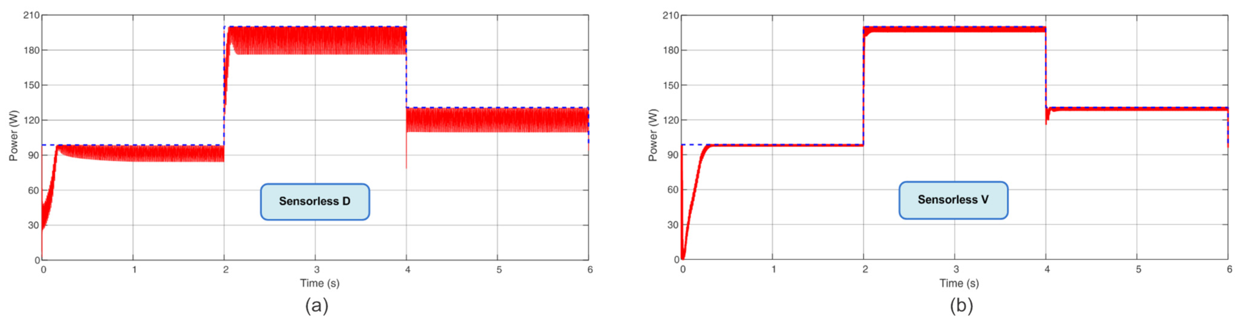
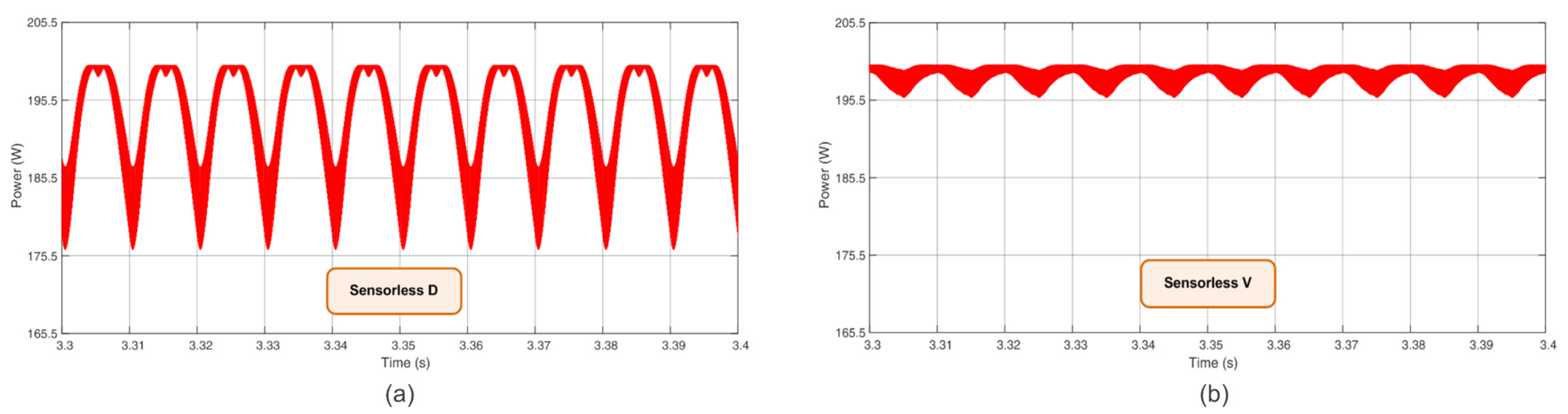
| Sensorless D | 94.65% |
| Sensorless V | 97.61% |
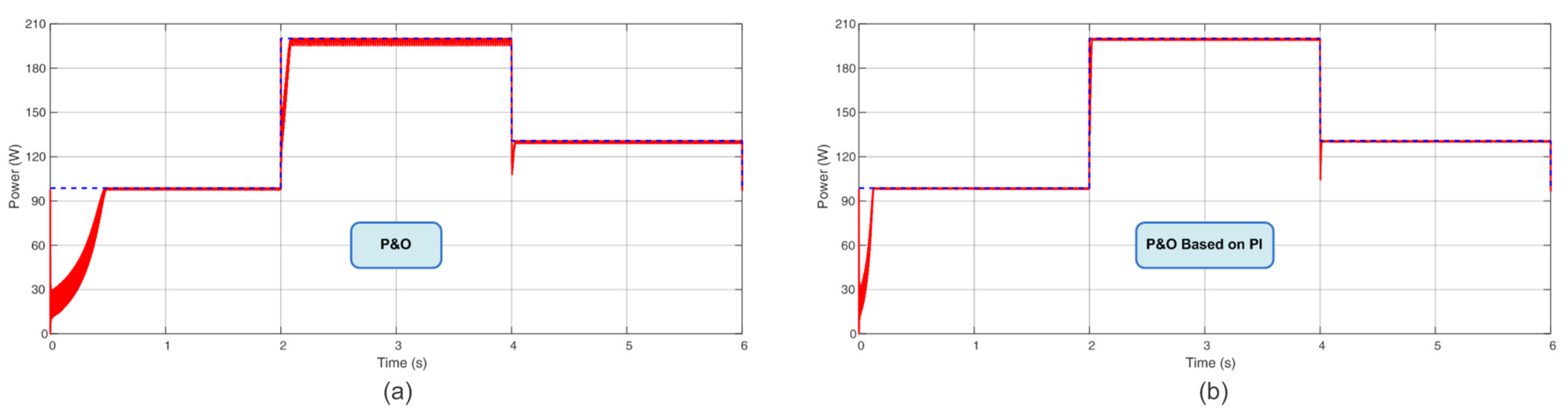
| P&O | 95.75% |
| P&O based on PI | 98.75% |
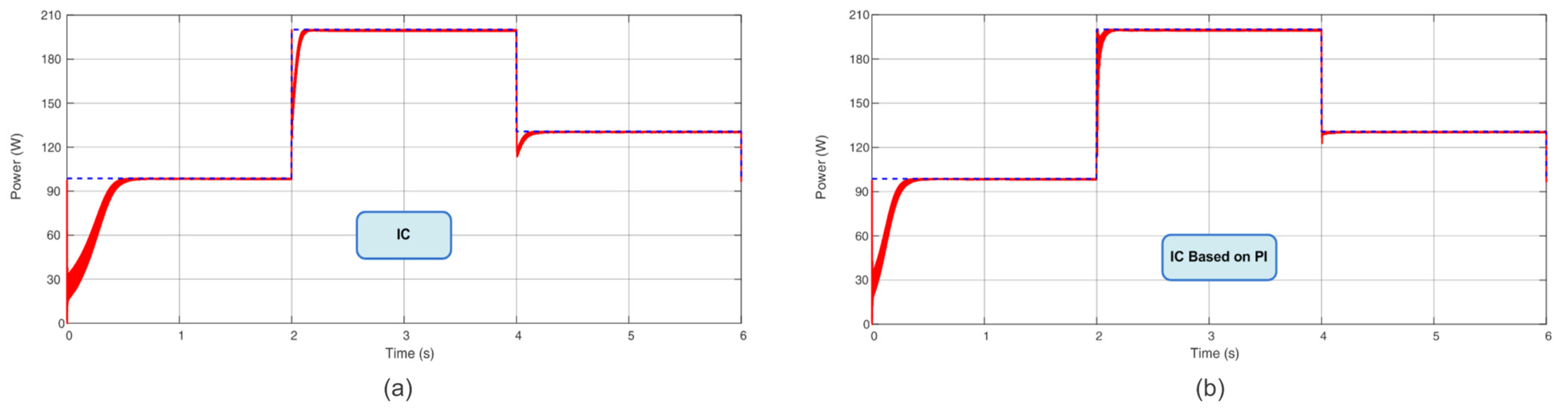
| IC | 95.85% |
| IC based on PI | 98.68% |
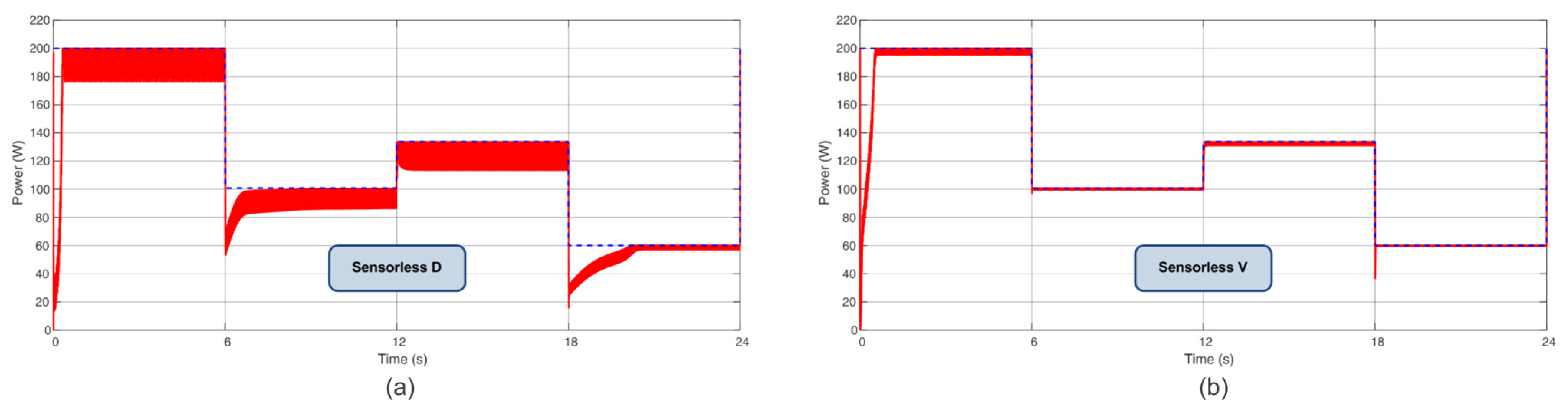
| Profile I | ||
| Irradiance | Temperature | Theoretical Power |
| 1000 W/m2 | 25 °C | 200.01 W |
| 500 W/m2 | 20 °C | 100.79 W |
| 700 W/m2 | 35 °C | 133.68 W |
| 300 W/m2 | 15 °C | 60.08 W |
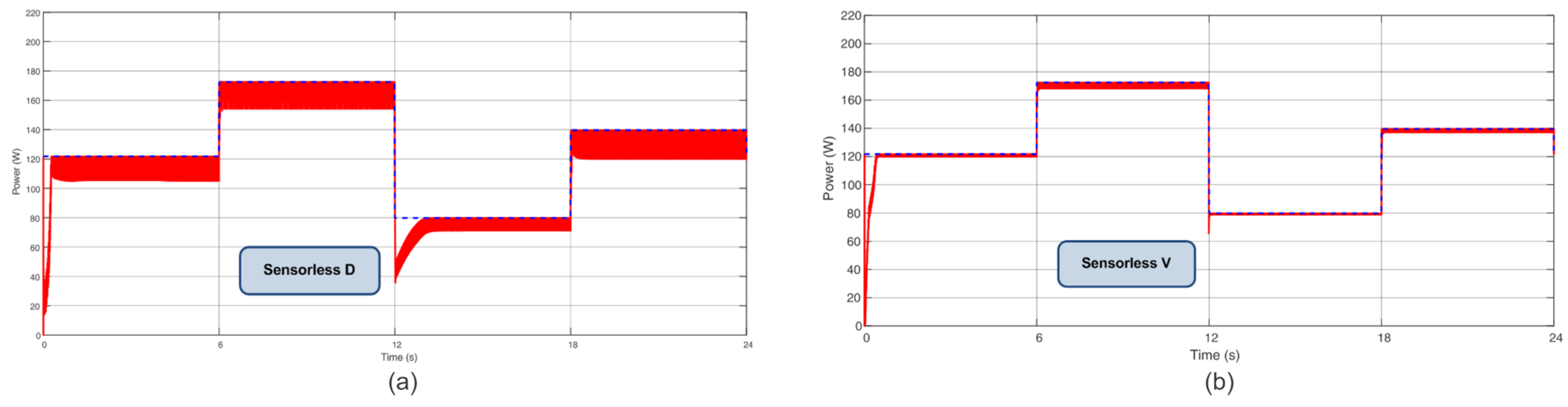
| Profile II | ||
| Irradiance | Temperature | Theoretical Power |
| 600 W/m2 | 20 °C | 121.74 W |
| 900 W/m2 | 35 °C | 172.47 W |
| 400 W/m2 | 20 °C | 79.80 W |
| 700 W/m2 | 25 °C | 139.62 W |
| Methods | Values |
|---|---|
| Constant Voltage [40] | 79.50% |
| Short Circuit Pulse [40] | 89.70% |
| Open Circuit Voltage [40] | 93.70% |
| LCASF [32] | 95.00% |
| LCA [32] | 96.00% |
| Proposed Current Sensorless V | 99.51% |
| FSCC [33] | 97.50% |
| Current Sensorless [41] | 92.10% |
| ASC-MPPT [42] | 96.20% |
| Hybrid FOCV-SCAM [29] | 99.70% |
| SC-MPC-MPPT [43] | 99.40% |
Disclaimer/Publisher’s Note: The statements, opinions and data contained in all publications are solely those of the individual author(s) and contributor(s) and not of MDPI and/or the editor(s). MDPI and/or the editor(s) disclaim responsibility for any injury to people or property resulting from any ideas, methods, instructions or products referred to in the content. |
© 2023 by the authors. Licensee MDPI, Basel, Switzerland. This article is an open access article distributed under the terms and conditions of the Creative Commons Attribution (CC BY) license (https://creativecommons.org/licenses/by/4.0/).
Share and Cite
de Brito, M.A.G.; Martines, G.M.S.; Volpato, A.S.; Godoy, R.B.; Batista, E.A. Current Sensorless Based on PI MPPT Algorithms. Sensors 2023, 23, 4587. https://doi.org/10.3390/s23104587
de Brito MAG, Martines GMS, Volpato AS, Godoy RB, Batista EA. Current Sensorless Based on PI MPPT Algorithms. Sensors. 2023; 23(10):4587. https://doi.org/10.3390/s23104587
Chicago/Turabian Stylede Brito, Moacyr A. G., Guilherme M. S. Martines, Anderson S. Volpato, Ruben B. Godoy, and Edson A. Batista. 2023. "Current Sensorless Based on PI MPPT Algorithms" Sensors 23, no. 10: 4587. https://doi.org/10.3390/s23104587