
PN Codes Estimation of Binary Phase Shift Keying Signal Based on Sparse Recovery for Radar Jammer
Abstract
:1. Introduction
- A novel PN codes estimation method based on NCTVR is proposed, and its corresponding optimization function is established.
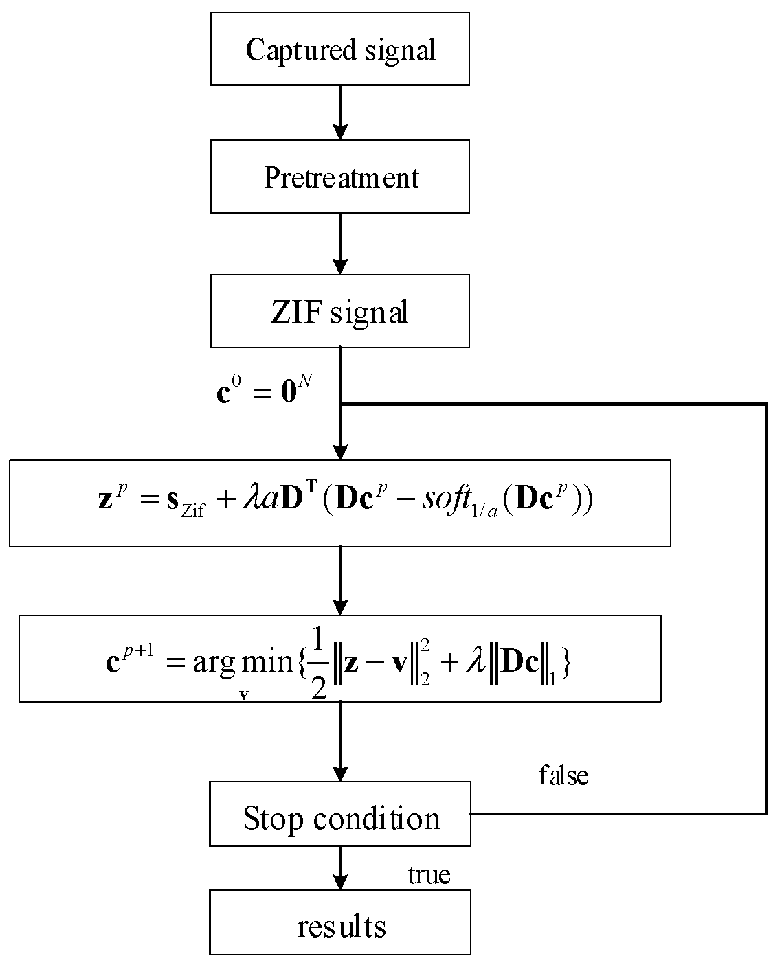
- An iterative algorithm based on the forward–backward splitting algorithm is proposed to solve the NCTVR.
- The proposed method is verified by numeric simulations and semiphysical tests.
2. Mathematical Model
3. PN Code Estimation Based on NCTVR
3.1. Pretreatment
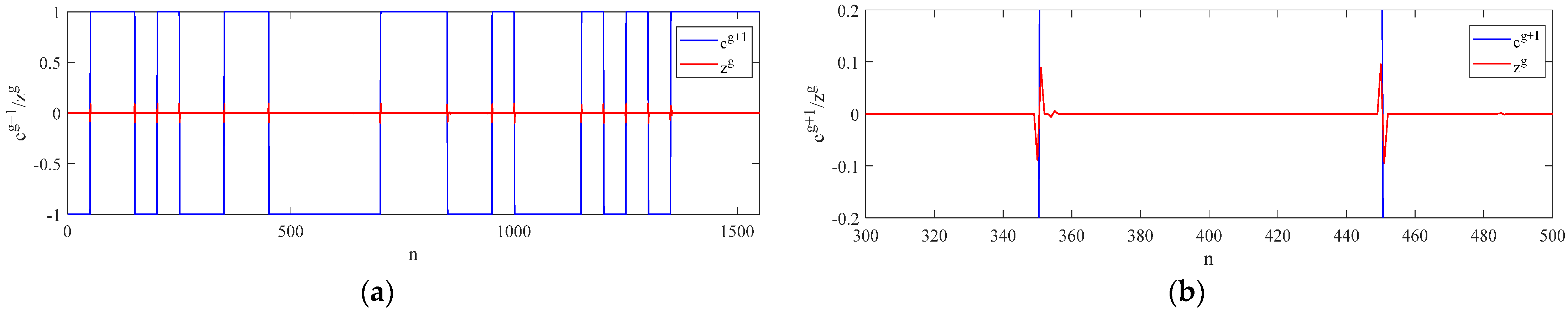
3.2. PN Code Estimation Based on NCTVR
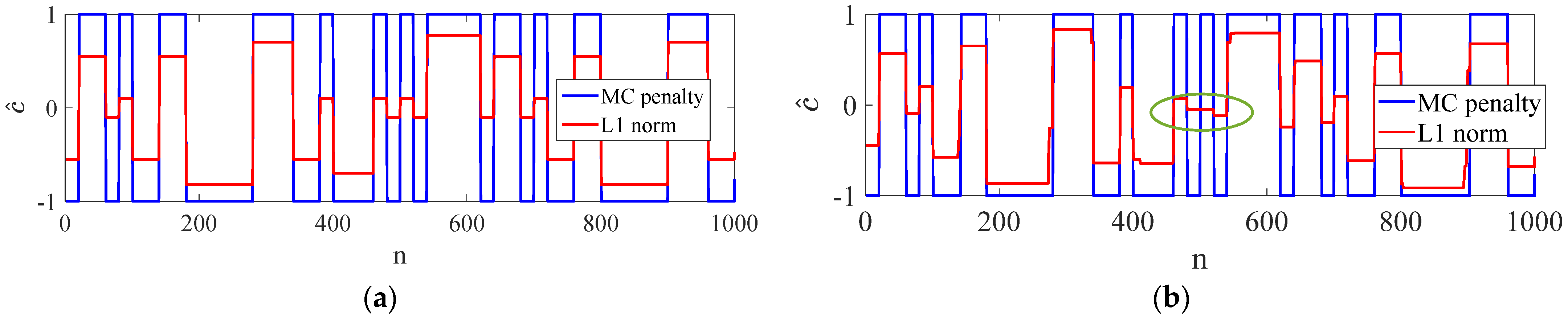
3.3. The Motivation behind the NCTVR
4. Performance of NCTVR
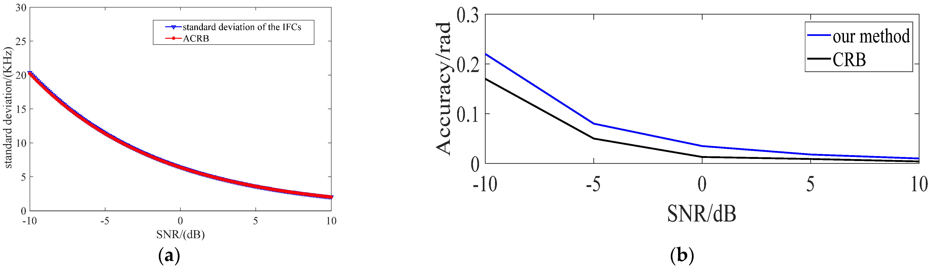
4.1. Variance of the Estimated Centre Frequency
4.2. Accuracy of The Estimated PN Codes
5. Simulations and Experiments
5.1. Simulations
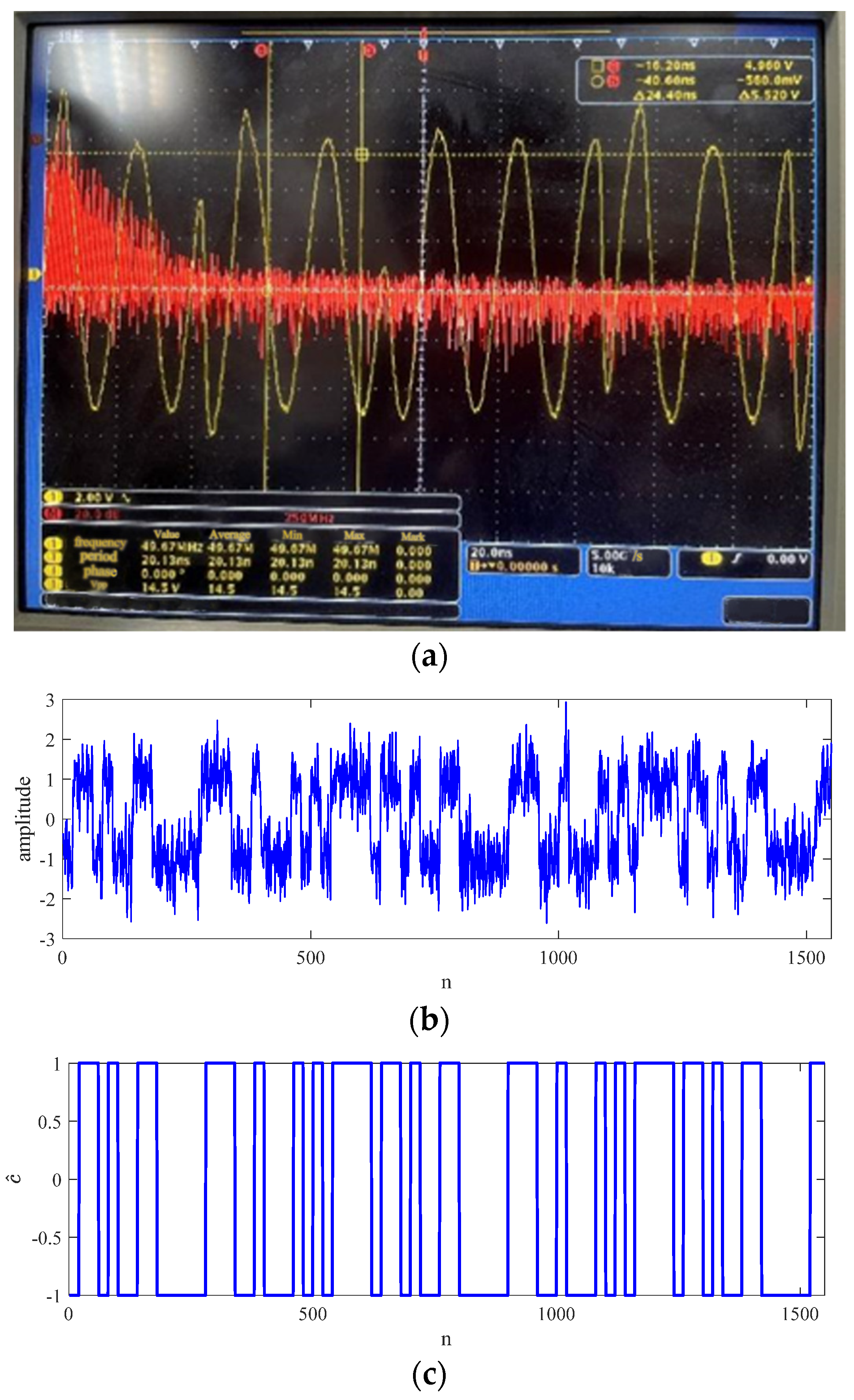
5.2. Experiments
6. Conclusions
Author Contributions
Funding
Institutional Review Board Statement
Informed Consent Statement
Data Availability Statement
Conflicts of Interest
References
- Cemil, A.; Ünlü, M. Analysis of ADAS Radars with Electronic Warfare Perspective. Sensors 2022, 22, 6142. [Google Scholar] [CrossRef] [PubMed]
- He, X.; Liao, K.; Peng, S.; Tian, Z.; Huang, J. Interrupted-Sampling Repeater Jamming-Suppression Method Based on a Multi-Stages Multi-Domains Joint Anti-Jamming Depth Network. Remote Sens. 2022, 14, 3445. [Google Scholar] [CrossRef]
- Cui, G.; Yu, X.; Yang, J.; Fu, Y.; Kong, L. An overview of waveform optimization methods for cognitive radar. J. Radars 2019, 8, 537–557. [Google Scholar]
- Hanbali, S.B.S.; Kastantin, R. A review of self-protection deceptive jamming against chirp radars. Int. J. Microw. Wirel. Technol. 2017, 9, 1853–1861. [Google Scholar] [CrossRef]
- Guo, R.; Ni, Y.; Liu, H.; Wang, F.; He, L. Signal diverse array radar for electronic warfare. IEEE Antennas Wirel. Propag. Lett. 2017, 16, 2906–2910. [Google Scholar] [CrossRef]
- Akay, O.; Boudreaux-Bartels, G.F. Fractional convolution and correlation via operator methods and an application to detection of linear FM signals. IEEE Trans. Signal Process. 2001, 49, 979–993. [Google Scholar] [CrossRef] [PubMed]
- Sun, Y.; Willett, P. Hough transform for long chirp detection. IEEE Trans. Aerosp. Electron. Syst. 2002, 38, 553–569. [Google Scholar] [CrossRef]
- Gu, T.; Liao, G.; Li, Y.; Guo, Y.; Huang, Y. Parameter estimate of multi-component LFM signals based on GAPCK-Science Direct. Digit. Signal Process. 2020, 100, 1–12. [Google Scholar] [CrossRef]
- Peleg, S.; Friedlander, B. The discrete polynomial-phase transform. IEEE Trans. Signal Process. 1995, 43, 1901–1914. [Google Scholar] [CrossRef]
- Jin, Y.; Ji, H.B. Cyclic Statistic Based Blind Parameter Estimation of BPSK and QPSK Signals. In Proceedings of the 2006 8th International Conference on Signal Processing, Guilin, China, 16–20 November 2006. [Google Scholar]
- Yang, W.; Yang, X.; Yin, K. Research on parameter estimation of MPSK signals based on the generalized second-order cyclic spectrum. In Proceedings of the 2014 XXXIth URSI General Assembly and Scientific Symposium, Beijing, China, 16–23 August 2014. [Google Scholar]
- Zhan, Y.; Duan, C. The application of stochastic resonance in parameter estimation for PSK signals. In Proceedings of the 2015 IEEE International Conference on Communication Software and Networks, Chengdu, China, 6–7 June 2015. [Google Scholar]
- Hu, Y.; Sawan, M. A fully integrated low-power BPSK demodulator for implantable medical devices. IEEE Trans. Circuits Syst. I Regul. Pap. 2005, 52, 2552–2562. [Google Scholar]
- Luo, Z.; Sonkusale, S. A Novel BPSK Demodulator for Biological Implants. IEEE Trans. Circuits Syst. I Regul. Pap. 2008, 55, 1478–1484. [Google Scholar]
- Nabovati, G.; Maymandi-Nejad, M. Ultra-low power BPSK demodulator for bio-implantable chips. IEICE Electron. Express 2010, 7, 1592–1596. [Google Scholar] [CrossRef] [Green Version]
- Wang, K.; Yan, X.; Zhu, Z.; Hao, X.; Li, P.; Yang, Q. Blind Estimation Methods for BPSK Signal Based on Duffing Oscillator. Sensors 2020, 20, 6412. [Google Scholar] [CrossRef]
- Yan, X.; Wang, K.; Liu, Q.; Hao, X.; Yu, H. Jamming Signal Design of Pseudo-code Phase Modulation Fuze Based on Duffing Oscillator. Acta Armamentarii 2022, 43, 729–736. [Google Scholar]
- Frigo, M.; Johnson, S.G. FFTW: An adaptive software architecture for the FFT. In Proceedings of the International Conference on Acoustic, Speech and Signal Processing, Seattle, WA, USA, 15 May 1998; Volume 3, pp. 1381–1384. [Google Scholar]
- Invertibility of Overlap-Add Processing. Available online: gauss256.github.io (accessed on 9 March 2022).
- Allen, R.L.; Mills, D.W. Signal Analysis: Times, Frequency, Scale and Structure; Wiley-Interscience: New York, NY, USA, 2004. [Google Scholar]
- Yang, Z.; Sun, I.; Guo, P.; Zhang, Y. A Method of Symbol Rate Estimation Based on Wavelet Transform for Digital Modulation Signals. In DEStech Transaction on Computer Science and Engineering; DEStech Publications, Inc.: Lancaster, PA, USA, 2017; ISBN 978-1-60595-504-9. [Google Scholar]
- Wang, Q.; Ge, Q. Blind estimation algorithm of parameters in PN sequence for DSSS-BPSK signals. In Proceedings of the 2012 International Conference on Wavelet Active Media Technology and Information Processing (ICWAMTIP), Chengdu, China, 17–19 December 2012; Institute of Electrical and Electronics Engineers (IEEE): New York, NY, USA, 2012; pp. 371–376. [Google Scholar]
- Guolin, L.; Min, H.; Ying, Z. PN Code Recognition and Parameter Estimation of PN-BPSK Signal Based on Synchronous Demodulation. In Proceedings of the 2007 8th International Conference on Electronic Measurement and Instruments, Xi’an, China, 16–18 August 2007; Institute of Electrical and Electronics Engineers (IEEE): New York, NY, USA, 2007; pp. 142–145. [Google Scholar]
- Duong, V.M.; Vesely, J.; Hubacek, P.; Janu, P.; Phan, N.G. Detection and Parameter Estimation Analysis of Binary Shift Keying Signals in High Noise Environments. Sensors 2022, 22, 3203. [Google Scholar] [CrossRef]
- Morelande, M.; Senadji, B.; Boashash, B.; Brisbane, Q.L.D. Complex-lag polynomial Wigner-Ville distribution. In Proceedings of the IEEE TENCON ’97. IEEE Region 10 Annual Conference. Speech and Image Technologies for Computing and Telecommunications, Brisbane, Australia, 4 December 1997. [Google Scholar]
- Daubechies, I.; Lu, J.; Wu, H.T. Synchrosqueezed wavelet transforms: An empirical mode decomposition-like tool. Appl. Comput. Harmon. Anal. 2011, 30, 243–261. [Google Scholar] [CrossRef] [Green Version]
- Stallone, A.; Cicone, A.; Materassi, M. New insights and best practices for the successful use of Empirical Mode Decomposition, Iterative Filtering and derived algorithms. Sci. Rep. 2020, 10, 15161. [Google Scholar] [CrossRef]
- Dragomiretskiy, K.; Zosso, D. Variational Mode Decomposition. IEEE Trans. Signal Process. 2013, 62, 531–544. [Google Scholar] [CrossRef]
- Huska, M.; Kang, S.H.; Lanza, A.; Morigi, S. A variational approach to additive image decomposition into structure, harmonic, and oscillatory components. SIAM J. Imaging Sci. 2021, 14, 1749–1789. [Google Scholar] [CrossRef]
- Chan, T.F.; Osher, S.; Shen, J. The digital TV filter and nonlinear denoising. IEEE Trans. Image Process. 2001, 10, 231–241. [Google Scholar] [CrossRef] [Green Version]
- Parekh, A.; Selesnick, I.W. Convex Denoising using Non-Convex Tight Frame Regularization. IEEE Signal Process. Lett. 2015, 22, 1786–1790. [Google Scholar] [CrossRef] [Green Version]
- Zou, J.; Shen, M.; Zhang, Y.; Li, H.; Liu, G.; Ding, S. Total Variation Denoising With Non-Convex Regularizers. IEEE Access 2018, 7, 4422–4431. [Google Scholar] [CrossRef]
- Selesnick, I. Sparse Regularization via Convex Analysis. IEEE Trans. Signal Process. 2017, 65, 4481–4494. [Google Scholar] [CrossRef]
- Cicone, A.; Huska, M.; Kang, S.-H.; Morigi, S. JOT: A Variational Signal Decomposition Into Jump, Oscillation and Trend. IEEE Trans. Signal Process. 2022, 70, 772–784. [Google Scholar] [CrossRef]
- Selesnick, I.; Lanza, A.; Morigi, S.; Sgallari, F. Non-convex Total Variation Regularization for Convex Denoising of Signals. J. Math. Imaging Vis. 2020, 62, 825–841. [Google Scholar] [CrossRef]
- Wang, S.; Selesnick, I.W.; Cai, G.; Ding, B.; Chen, X. Synthesis versus analysis priors via generalized minimax-concave penalty for sparsity-assisted machinery fault diagnosis. Mech. Syst. Signal Process. 2019, 127, 202–233. [Google Scholar] [CrossRef]
- Aboutanios, E.; Mulgrew, B. Iterative frequency estimation by interpolation on Fourier coefficients. IEEE Trans. Signal Process. 2005, 53, 1237–1242. [Google Scholar] [CrossRef]


| Existing Methods | Principle | Limitations |
|---|---|---|
| Methods proposed in [10,11,12] and [18,19,20,21] | They adopt time frequency analysis to estimate the chip rate and carrier frequency of the BPSK signal | They are unable to estimate the PN codes. |
| Two-stage method proposed in [24] | It adopts the cross correlation to estimate the PN codes of the BPSK signal in serious SNR. | It is only suitable for Barker codes 7, 11 and 13. |
| Method proposed in [23] | It adopts matrix eigen decomposition to estimate the PN codes of the BPSK signal. | It needs to know the chip rate and period of the PN code as a priori |
| Method proposed in [16] | It uses the state changes of the duffing oscillator to estimate the PN codes of the BPSK signal in serious SNR | It only detects the polarity changes of the PN codes and needs to know the polarity of starting symbol as a priori. |
| Our two-stage method. | It uses the sparsity of the PN codes in time domain to estimate the PN codes of the BPSK signal in serious SNR | \ |
Disclaimer/Publisher’s Note: The statements, opinions and data contained in all publications are solely those of the individual author(s) and contributor(s) and not of MDPI and/or the editor(s). MDPI and/or the editor(s) disclaim responsibility for any injury to people or property resulting from any ideas, methods, instructions or products referred to in the content. |
© 2023 by the authors. Licensee MDPI, Basel, Switzerland. This article is an open access article distributed under the terms and conditions of the Creative Commons Attribution (CC BY) license (https://creativecommons.org/licenses/by/4.0/).
Share and Cite
Peng, B.; Chen, Q. PN Codes Estimation of Binary Phase Shift Keying Signal Based on Sparse Recovery for Radar Jammer. Sensors 2023, 23, 554. https://doi.org/10.3390/s23010554
Peng B, Chen Q. PN Codes Estimation of Binary Phase Shift Keying Signal Based on Sparse Recovery for Radar Jammer. Sensors. 2023; 23(1):554. https://doi.org/10.3390/s23010554
Chicago/Turabian StylePeng, Bo, and Qile Chen. 2023. "PN Codes Estimation of Binary Phase Shift Keying Signal Based on Sparse Recovery for Radar Jammer" Sensors 23, no. 1: 554. https://doi.org/10.3390/s23010554