Figure 1.
The structure of the signal processing algorithm in a MIMO communication system.
Figure 1.
The structure of the signal processing algorithm in a MIMO communication system.
Figure 2.
SER versus signal-noise ratio per bit for a 64-QAM signal in a channel with slow Rayleigh fading in the absence of IQ imbalance and DC offset using Equations (5) and (6) and from [
31].
Figure 2.
SER versus signal-noise ratio per bit for a 64-QAM signal in a channel with slow Rayleigh fading in the absence of IQ imbalance and DC offset using Equations (5) and (6) and from [
31].
Figure 3.
SER of 4-QAM versus SNR per bit for the algorithms, described by Equations (5)–(9) and (12) with polynomial approximation of the first order for different values of and .
Figure 3.
SER of 4-QAM versus SNR per bit for the algorithms, described by Equations (5)–(9) and (12) with polynomial approximation of the first order for different values of and .
Figure 4.
SER of 4-QAM versus SNR per bit for the algorithms, described by Equations (5)–(9) and (12) with polynomial approximation of the zero order—(a), zero and first orders—(b).
Figure 4.
SER of 4-QAM versus SNR per bit for the algorithms, described by Equations (5)–(9) and (12) with polynomial approximation of the zero order—(a), zero and first orders—(b).
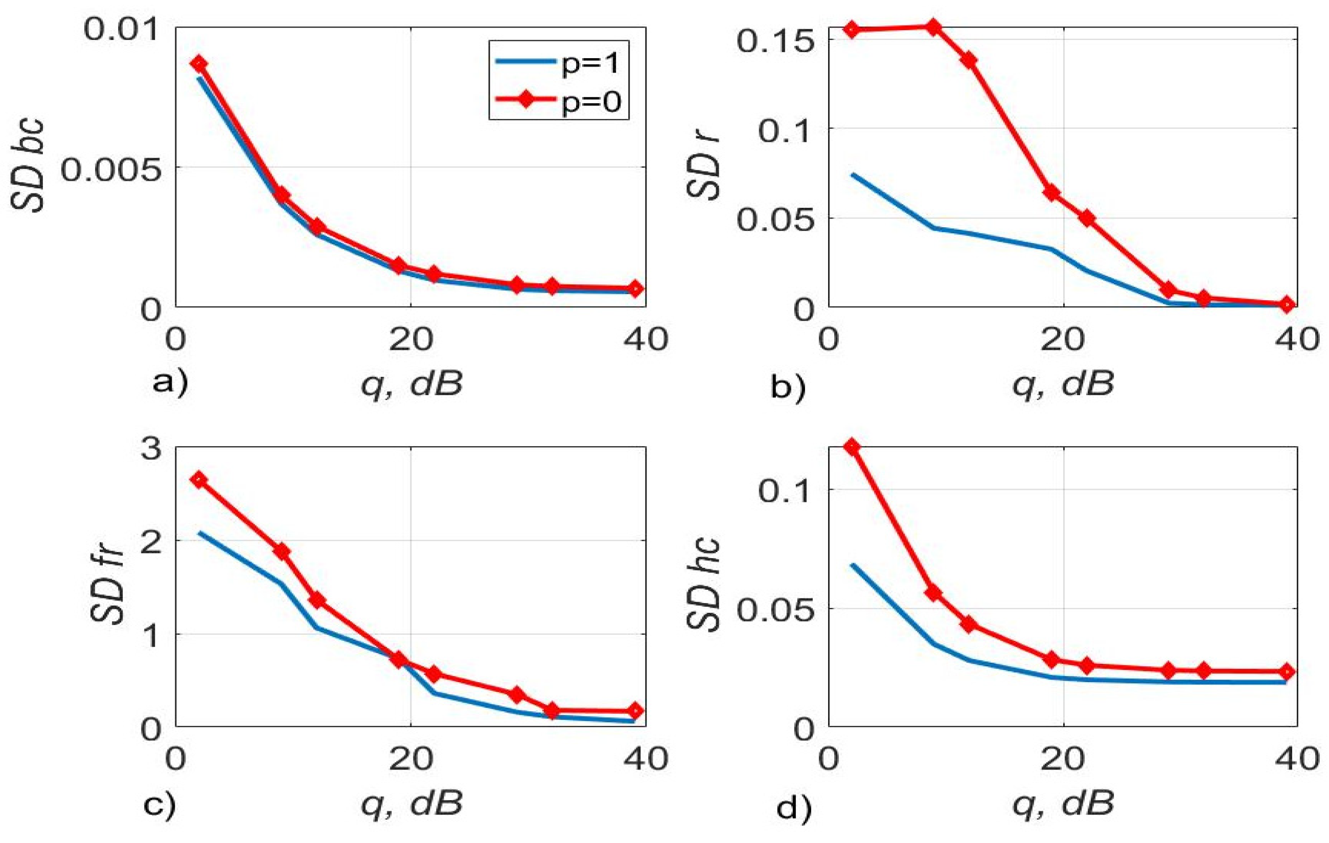
Figure 5.
The SD of estimating DC offset (SD bc)—(a), amplitude imbalance (SD r)—(b), phase imbalance (SD fr) (deg)—(c) and channel gains (SD hc)—(d) versus SNR per bit, the test signal was modulated by 4-QAM and the algorithms, described by Equations (5)–(9) and (12) with , was used.
Figure 5.
The SD of estimating DC offset (SD bc)—(a), amplitude imbalance (SD r)—(b), phase imbalance (SD fr) (deg)—(c) and channel gains (SD hc)—(d) versus SNR per bit, the test signal was modulated by 4-QAM and the algorithms, described by Equations (5)–(9) and (12) with , was used.
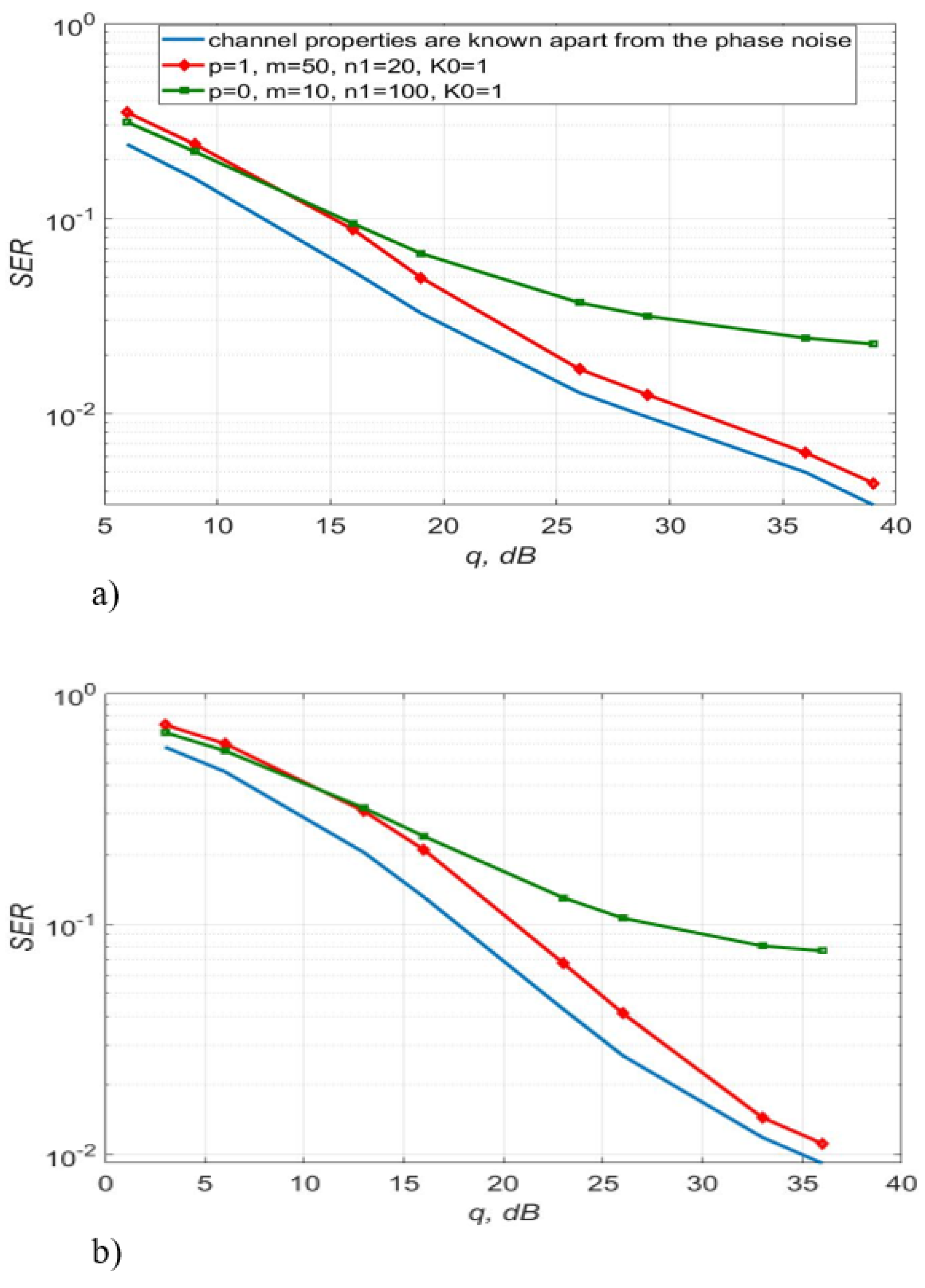
Figure 6.
SER of 16-QAM—(a), 64-QAM—(b) versus SNR for the algorithms, described by Equations (5)–(9) and (12) with polynomial approximation of zero and the first order.
Figure 6.
SER of 16-QAM—(a), 64-QAM—(b) versus SNR for the algorithms, described by Equations (5)–(9) and (12) with polynomial approximation of zero and the first order.
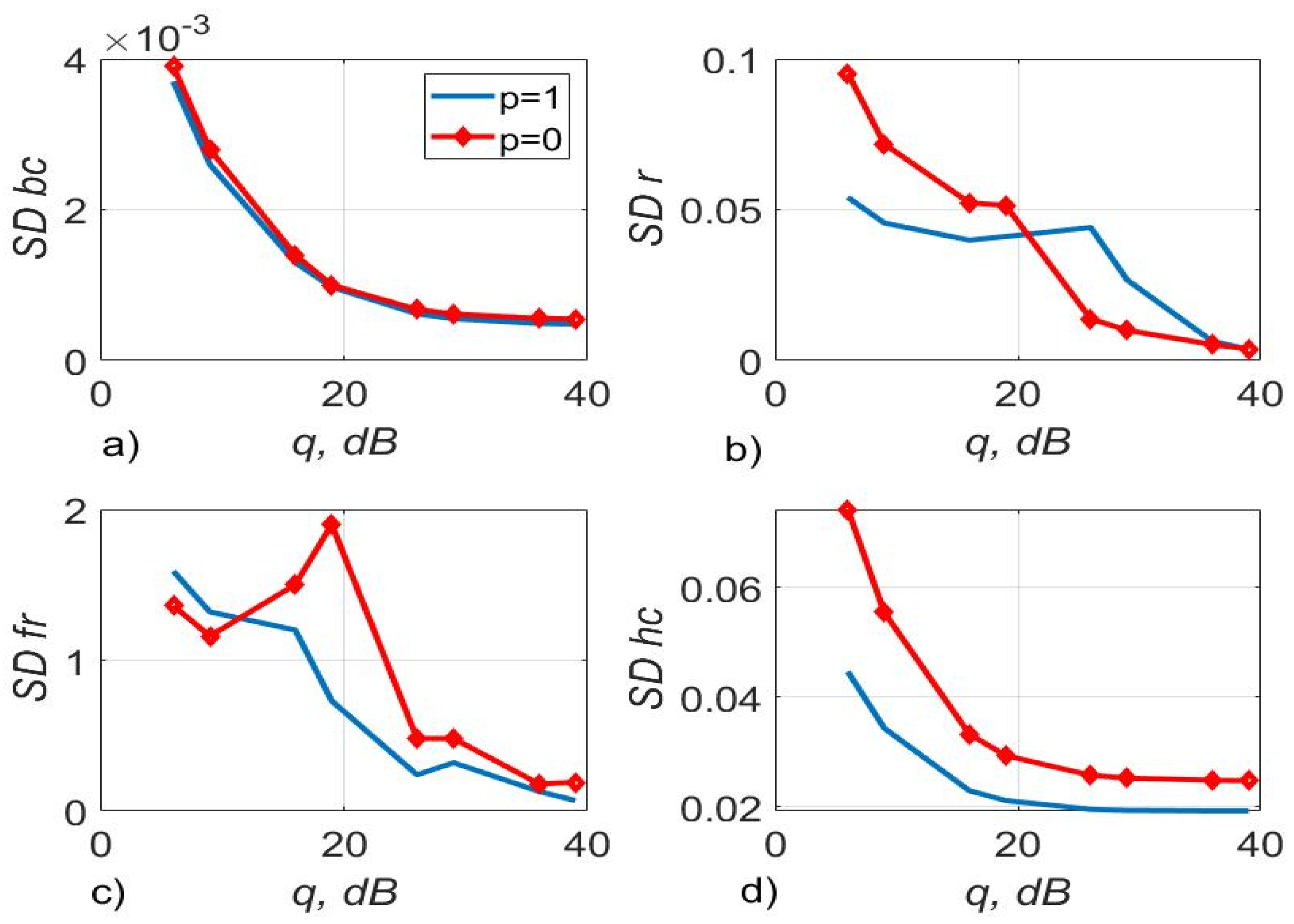
Figure 7.
The SD of estimating DC offset—(a), amplitude imbalance—(b), phase imbalance (deg)—(c), and channel gains—(d) versus SNR per bit, the test signal was modulated by 16-QAM and the algorithms, described by Equations (5)–(9) and (12) with , was used.
Figure 7.
The SD of estimating DC offset—(a), amplitude imbalance—(b), phase imbalance (deg)—(c), and channel gains—(d) versus SNR per bit, the test signal was modulated by 16-QAM and the algorithms, described by Equations (5)–(9) and (12) with , was used.
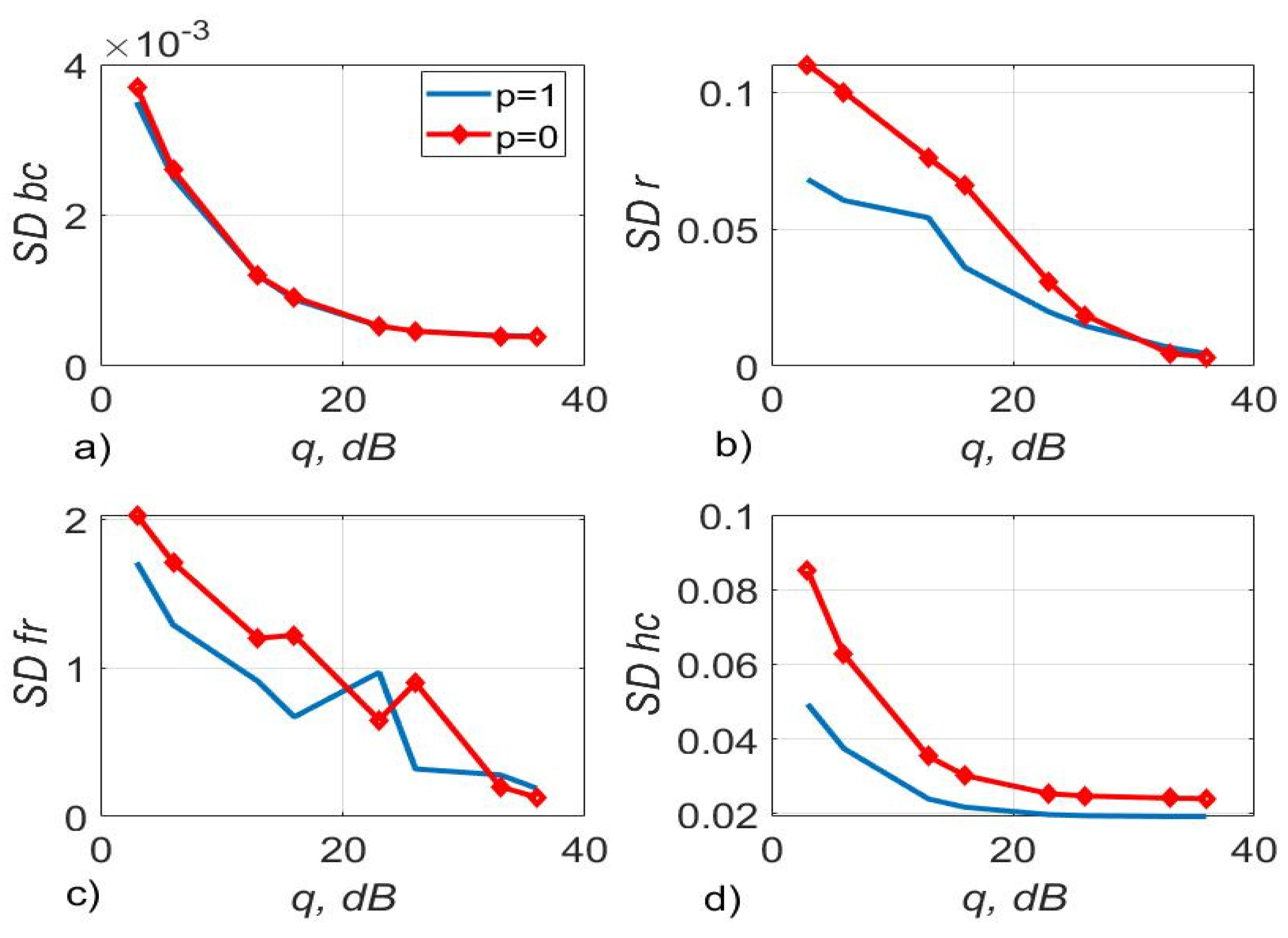
Figure 8.
The SD of estimating DC offset—(a), amplitude imbalance—(b), phase imbalance (deg)—(c), and channel gains—(d) versus SNR per bit, the test signal was modulated by 64-QAM and the algorithms, described by Equations (5)–(9) and (12) with , was used.
Figure 8.
The SD of estimating DC offset—(a), amplitude imbalance—(b), phase imbalance (deg)—(c), and channel gains—(d) versus SNR per bit, the test signal was modulated by 64-QAM and the algorithms, described by Equations (5)–(9) and (12) with , was used.
Figure 9.
Constellations of the 64-QAM (SNR is 26 dB per bit) at the input of the compensator—(a); at the output of the compensator which uses the algorithms, described by Equations (5)–(9) and (12) with —(b); —(c).
Figure 9.
Constellations of the 64-QAM (SNR is 26 dB per bit) at the input of the compensator—(a); at the output of the compensator which uses the algorithms, described by Equations (5)–(9) and (12) with —(b); —(c).
Figure 10.
Channel gains and their estimation based on the test signal versus time: the algorithms, described by Equations (5)–(9) and (12) with was used—(a), SNR = 26 dB; the enlarged fragment of “a)” part of the Figure—(b).
Figure 10.
Channel gains and their estimation based on the test signal versus time: the algorithms, described by Equations (5)–(9) and (12) with was used—(a), SNR = 26 dB; the enlarged fragment of “a)” part of the Figure—(b).
Figure 11.
Channel gains and their estimation based on the test signal versus time: the algorithms, described by Equations (5)–(9) and (12) with was used—(a), SNR = 26 dB; the enlarged fragment of (a,b).
Figure 11.
Channel gains and their estimation based on the test signal versus time: the algorithms, described by Equations (5)–(9) and (12) with was used—(a), SNR = 26 dB; the enlarged fragment of (a,b).
Figure 12.
Extrapolated values of the channel gains versus time for and —(a), —(b), SNR = 26 dB.
Figure 12.
Extrapolated values of the channel gains versus time for and —(a), —(b), SNR = 26 dB.
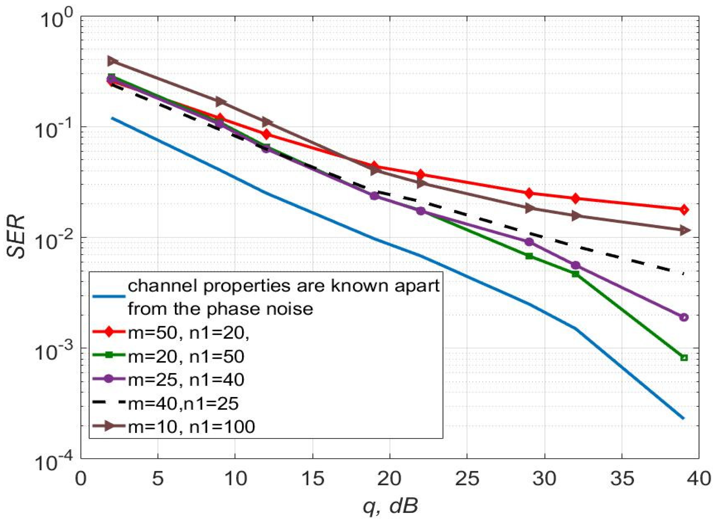
Figure 13.
SER of 4-QAM versus SNR per bit; the algorithms, described by Equations (5)–(9) and (12) with was used for and different values of and .
Figure 13.
SER of 4-QAM versus SNR per bit; the algorithms, described by Equations (5)–(9) and (12) with was used for and different values of and .
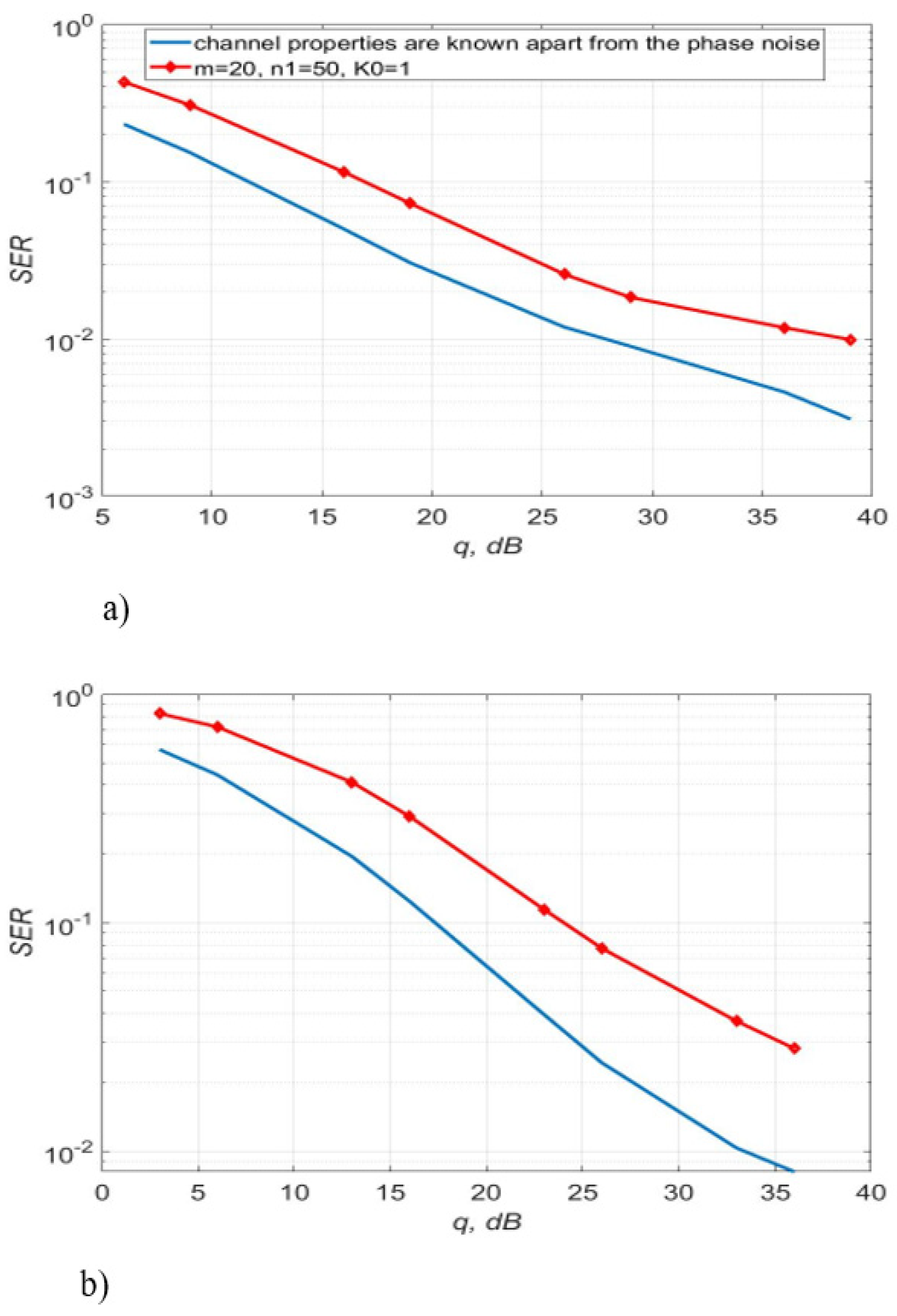
Figure 14.
SER of 16-QAM (a), 64-QAM (b) versus SNR per bit: the algorithms, described by Equations (5)–(9) and (12), .
Figure 14.
SER of 16-QAM (a), 64-QAM (b) versus SNR per bit: the algorithms, described by Equations (5)–(9) and (12), .
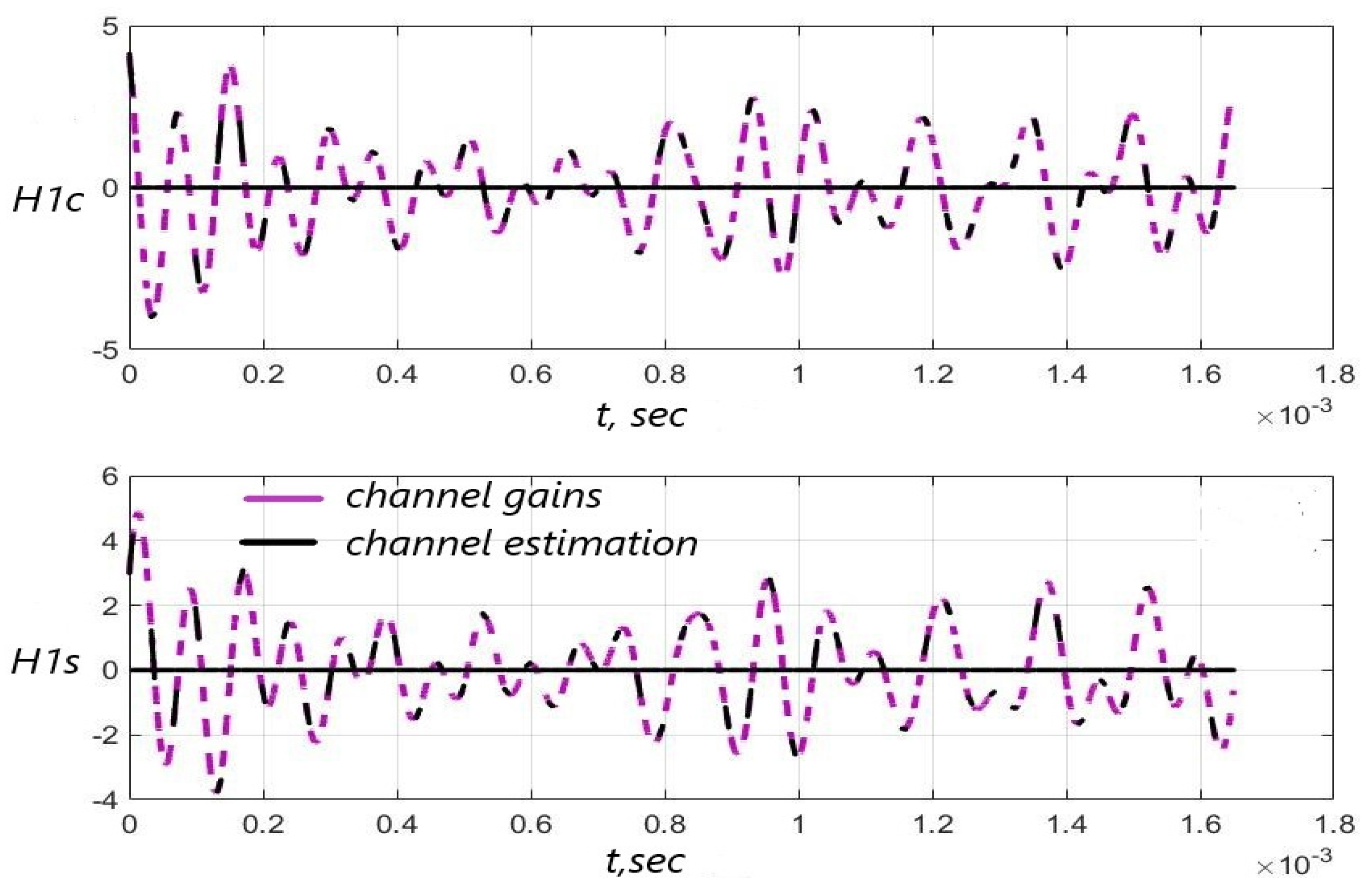
Figure 15.
Channel gains and their estimation based on the test signal versus time: , , SNR = 26 dB.
Figure 15.
Channel gains and their estimation based on the test signal versus time: , , SNR = 26 dB.
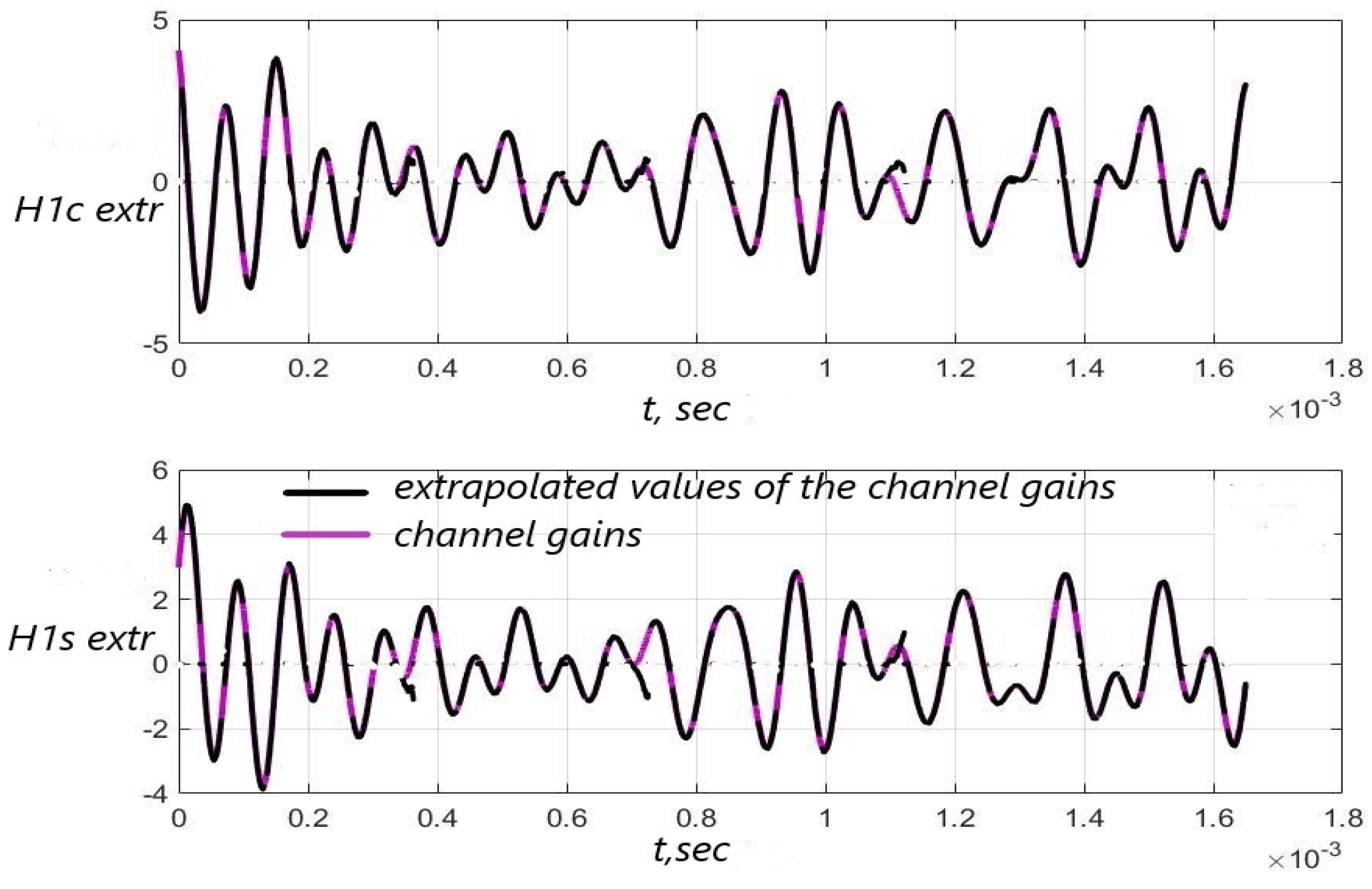
Figure 16.
Extrapolated values of the channel gains versus time for and , SNR = 26 dB.
Figure 16.
Extrapolated values of the channel gains versus time for and , SNR = 26 dB.
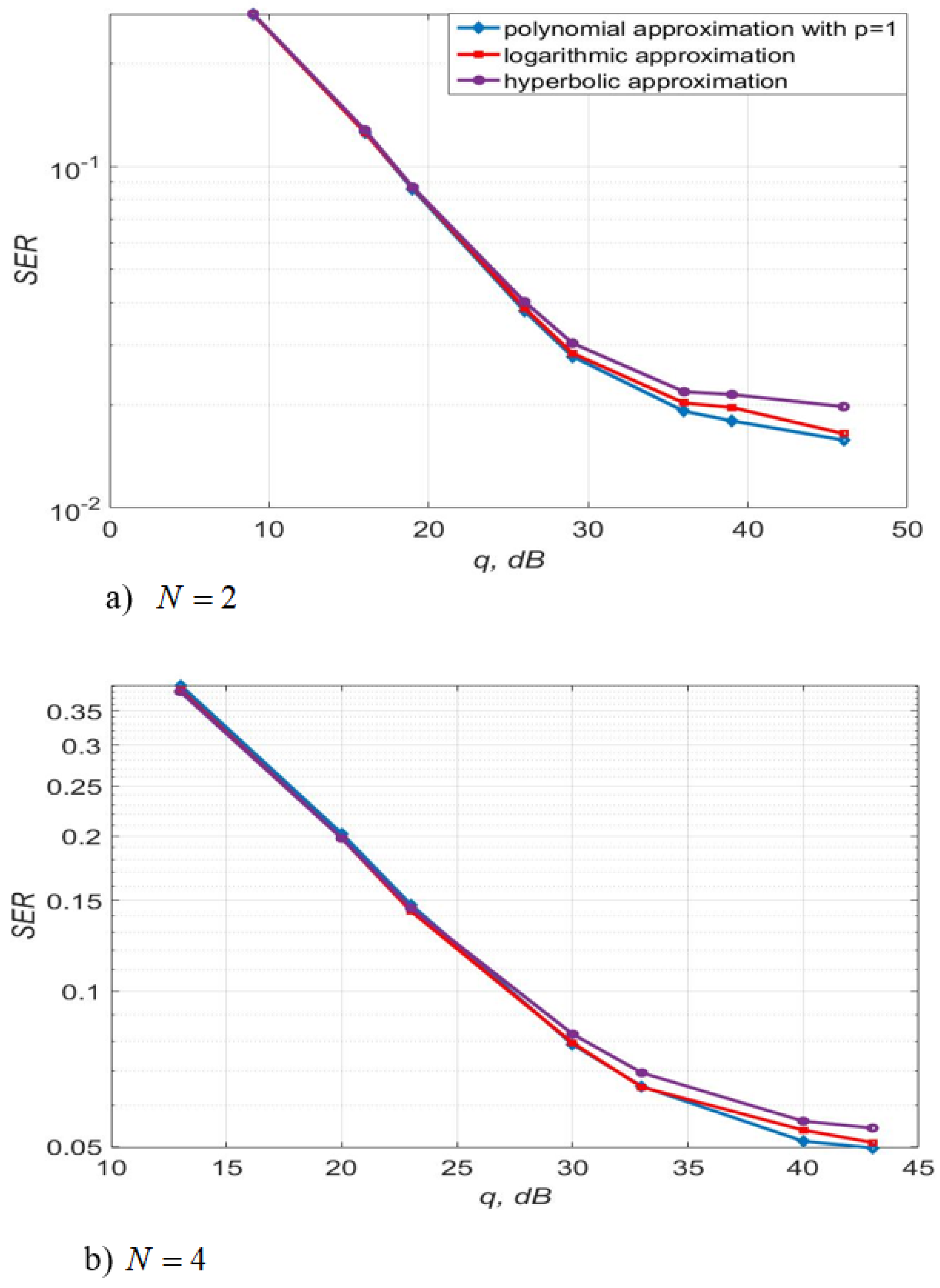
Figure 17.
SER of 4-QAM versus SNR per bit for different approximating structures for MIMO systems.
Figure 17.
SER of 4-QAM versus SNR per bit for different approximating structures for MIMO systems.
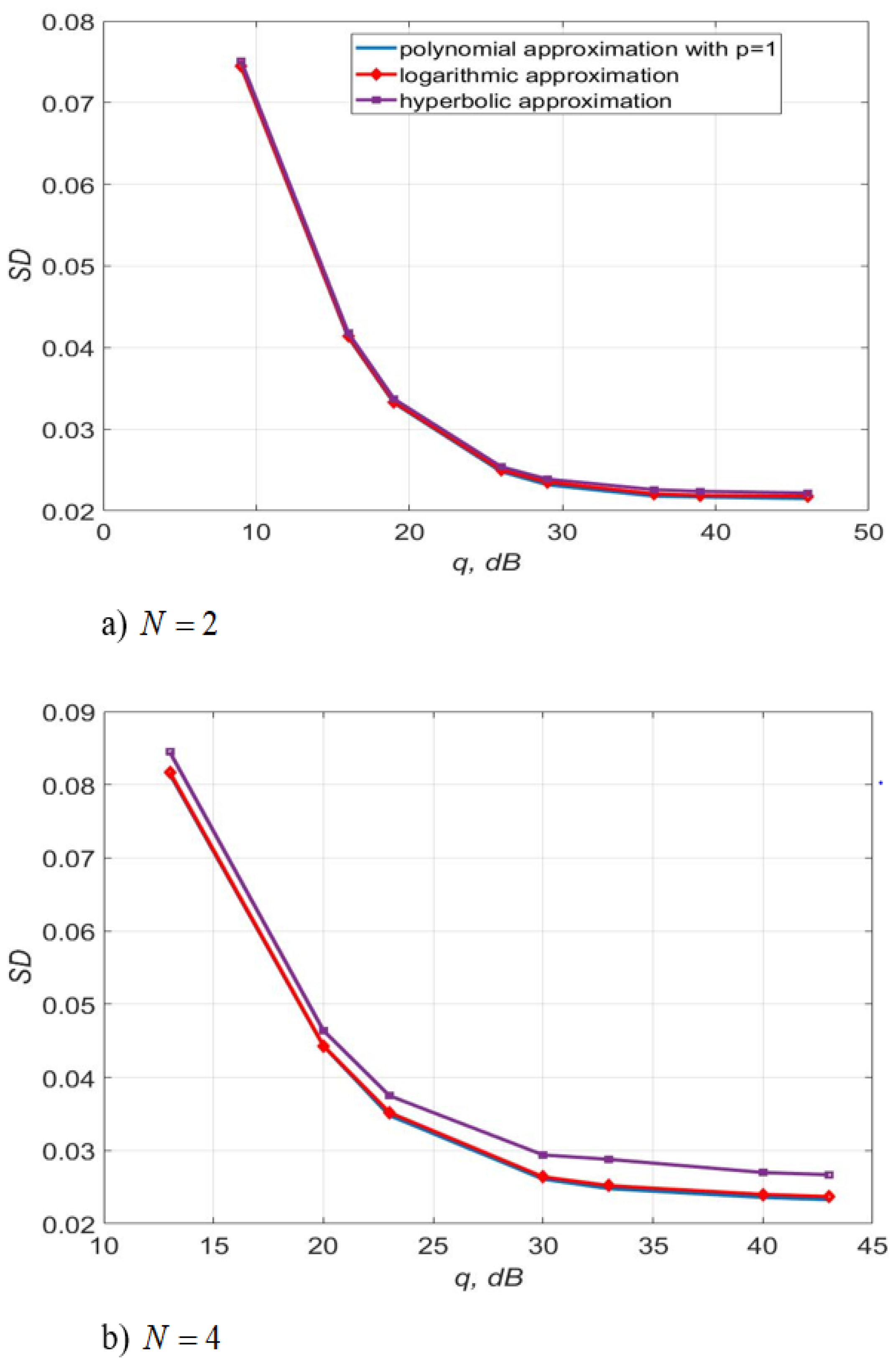
Figure 18.
The SD of the channel gains estimation versus SNR per bit for different approximating structures for MIMO systems.
Figure 18.
The SD of the channel gains estimation versus SNR per bit for different approximating structures for MIMO systems.
Table 1.
Symbols, vectors, and matrices used in this work.
Table 1.
Symbols, vectors, and matrices used in this work.
| Notation of Symbols and Matrices | Description |
|---|
| ()—dimensional real vector space |
| Expected value |
| Number of transmitting and receiving antennas |
| The number of the transmitting antenna. |
| The number of the receiving antenna. |
| Discrete time |
| In-phase and quadrature components (IQ) of the received signal |
| Elements of vectors |
| In-phase and quadrature components of the channel matrix |
| Elements of the matrix |
| Elements of the matrix |
| IQ vectors of the DC offset |
| Elements of vectors |
| The vector of information symbols M-QAM or symbols of the test signal |
| Elements of the vector |
| The row vector the form of which is determined by the type of the approximation |
| Vectors of coefficients of approximation of elements |
| , | Elements of vectors |
| Vectors of coefficients of approximation of elements |
| , | Elements of vectors |
| Harmonic amplitudes in the trigonometric approximation from [31] |
| Approximation order |
| The length of the test signal |
| Number of test signal transmission sessions |
| The length of the channel extrapolation interval |
Table 2.
Parameters of the channel and signal distortion in the direct conversion receiver.
Table 2.
Parameters of the channel and signal distortion in the direct conversion receiver.
| Parameter | Description |
|---|
| Amplitude imbalance between IQ components at the -th receiving antenna |
| Phase imbalance between IQ components at the -th receiving antenna |
| DC offsets of IQ components at -th receiving antenna |
| The frequency offset after demodulation |
| Time-varying channel gains |
| Phase of the signal |
| Phase noise |
| An initial random phase |
| The duration of signal symbols M-QAM |
Table 3.
Calculation of the computational complexity of the algorithm [
31] for SISO systems.
Table 3.
Calculation of the computational complexity of the algorithm [
31] for SISO systems.
| Calculated Member | Number of Operations |
|---|
| |
| |
| |
| |
| 2 |
| 8 |
| |
| |
| |
| |
| |
| The algorithm performs operations in iterations |
Table 4.
Calculation of the computational complexity of the algorithms, described by Equations (5), (8) and (9) for MIMO systems with transmitting and receiving antennas.
Table 4.
Calculation of the computational complexity of the algorithms, described by Equations (5), (8) and (9) for MIMO systems with transmitting and receiving antennas.
| Calculated Member | Number of Operations |
|---|
| |
| |
| |
| |
| |
Total number of operations:
|
Table 5.
The computational complexity of the algorithms, described by Equations (5), (8) and (9), and from [
31].
Table 5.
The computational complexity of the algorithms, described by Equations (5), (8) and (9), and from [
31].
| The Order of Approximation | Algorithms, Described by Equations (5), (8) and (9) | Algorithm from [31] |
|---|
| | - |
| | |
| - | |
| - | |
| - | |
Table 6.
SER of 4-QAM versus SNR per bit for .
Table 6.
SER of 4-QAM versus SNR per bit for .
|
q, dB | 2 | 9 | 12 | 19 | 22 | 29 | 32 | 39 |
|---|
| Polynomial approximation, |
| SER | | | | | | | | |
| Logarithmic approximation |
| SER | | | | | | | | |
| Hyperbolic approximation |
| SER | | | | | | | | |
Table 7.
SER of 16-QAM versus SNR per bit for .
Table 7.
SER of 16-QAM versus SNR per bit for .
|
q, dB
| 6 | 9 | 16 | 19 | 26 | 29 | 36 | 39 |
|---|
| Polynomial approximation, |
| SER | | | | | | | | |
| Logarithmic approximation |
| SER | | | | | | | | |
| Hyperbolic approximation |
| SER | | | | | | | | |
Table 8.
SER of 64-QAM versus SNR per bit for .
Table 8.
SER of 64-QAM versus SNR per bit for .
| q, dB | 3 | 6 | 13 | 16 | 23 | 26 | 33 | 36 |
|---|
| Polynomial approximation, |
| SER | | | | | | | | |
| Logarithmic approximation |
| SER | | | | | | | | |
| Hyperbolic approximation |
| SER | | | | | | | | |


