
A Hybrid Water Balance Machine Learning Model to Estimate Inter-Annual Rainfall-Runoff


Abstract
:1. Introduction
2. Material and Methods
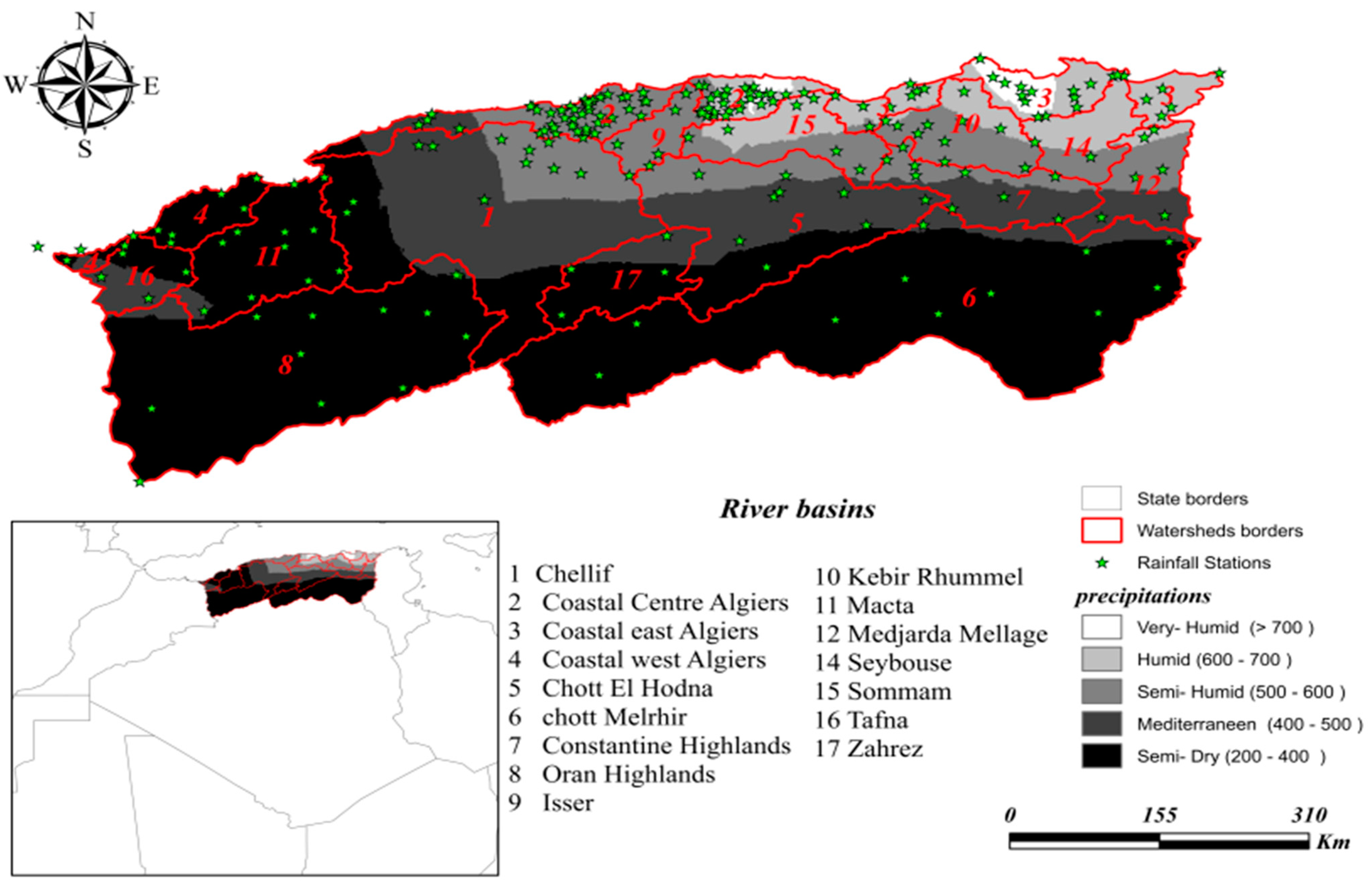
2.1. Study Area and Data
2.2. Water Balance Model
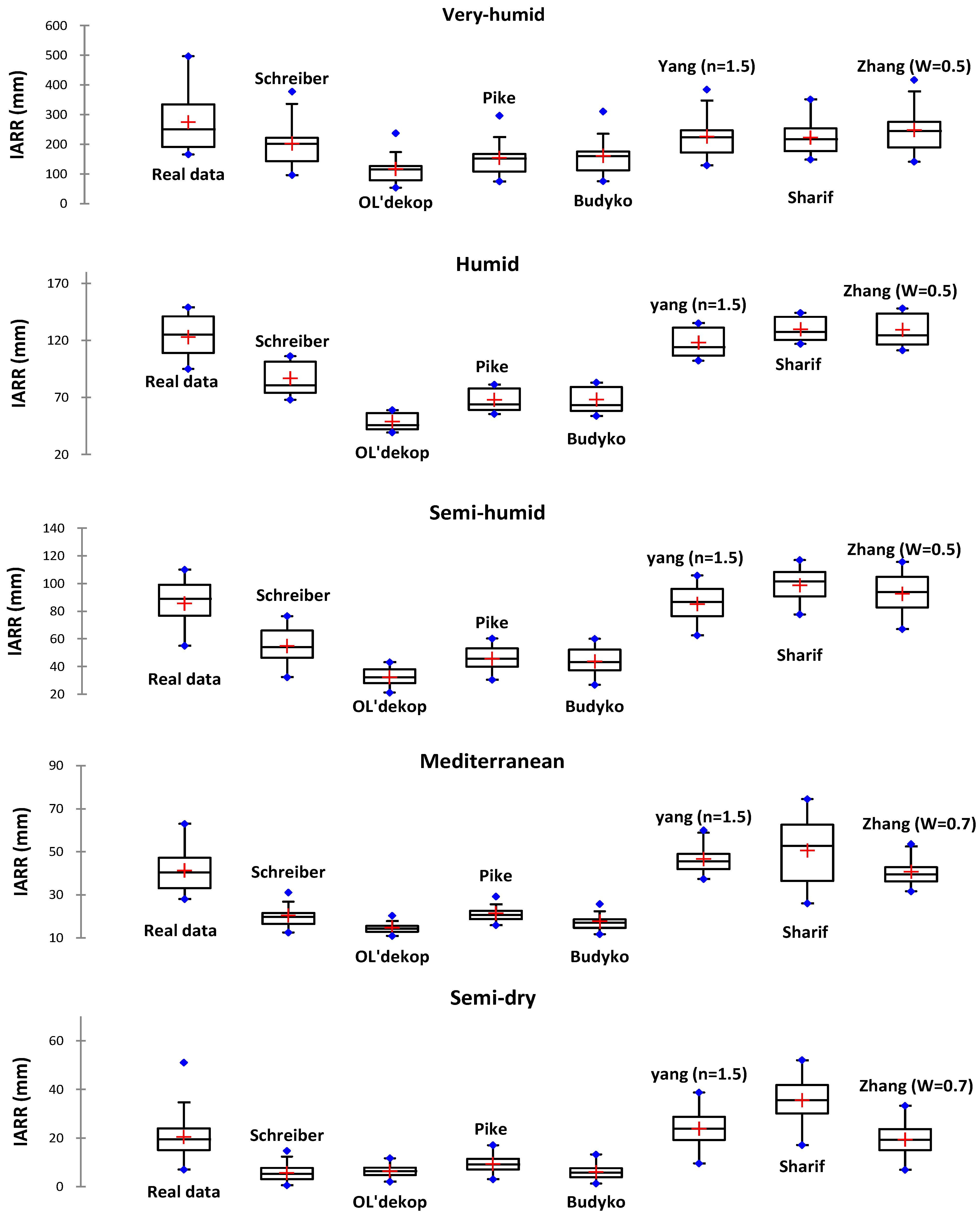
2.2.1. Schreiber
2.2.2. Ol’Dekop
2.2.3. Pike
2.2.4. Budyko
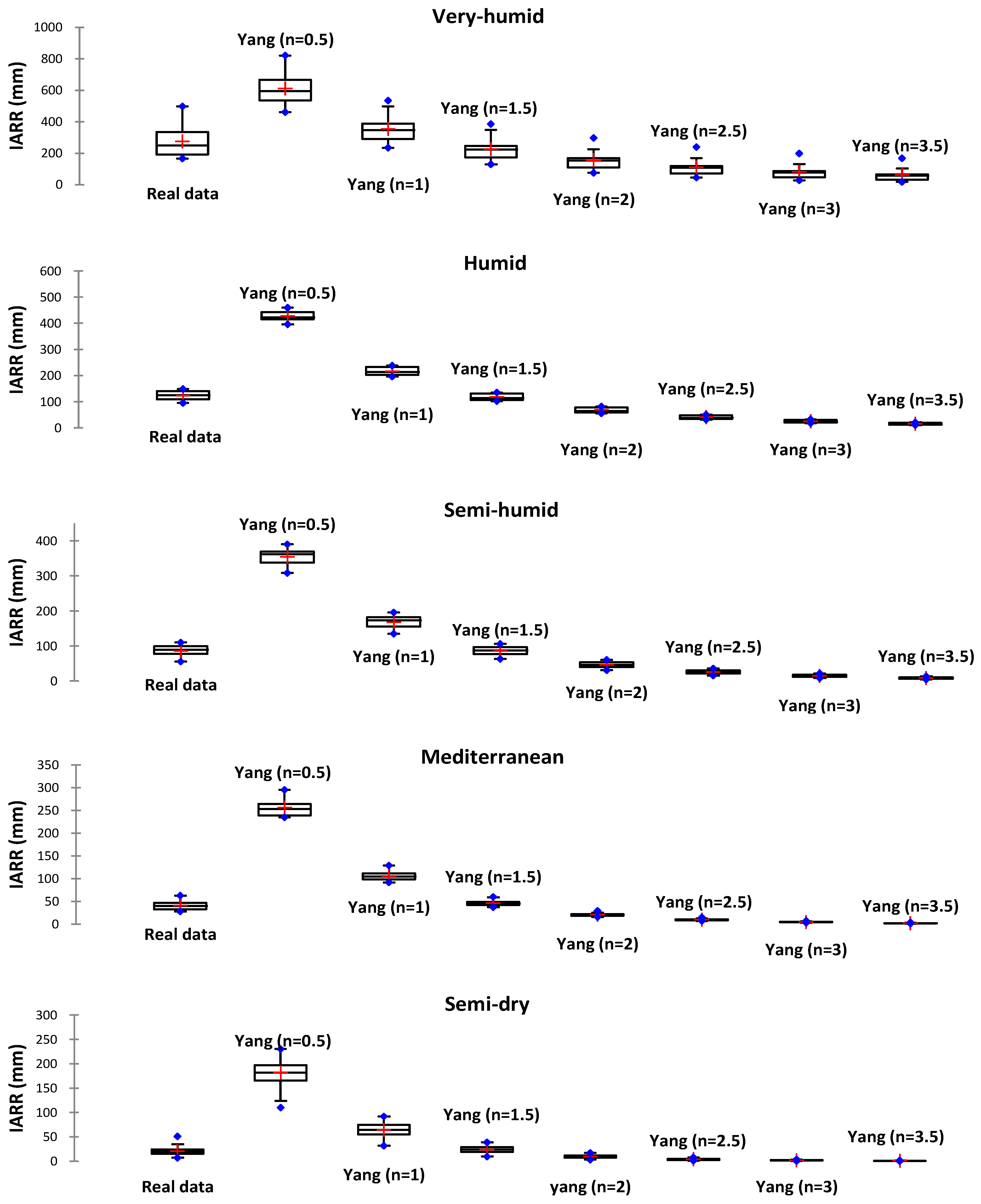
2.2.5. Yang
2.2.6. Sharif
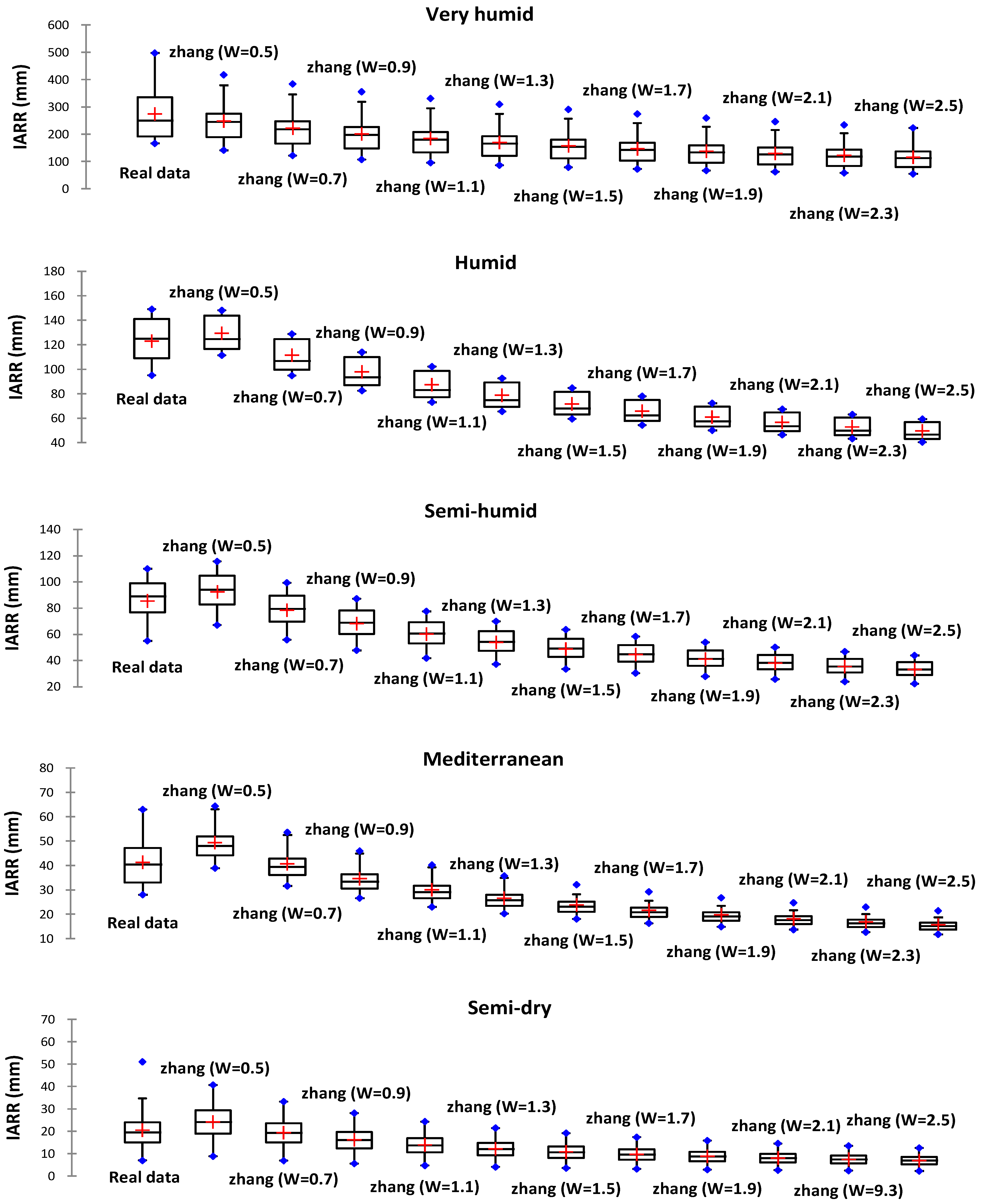
2.2.7. Zhang
2.3. Machine Learning Models
2.3.1. Multiple Regression Model (MR)
2.3.2. Classification and Regression Tree Model (CART)
3. Results
3.1. Data Description
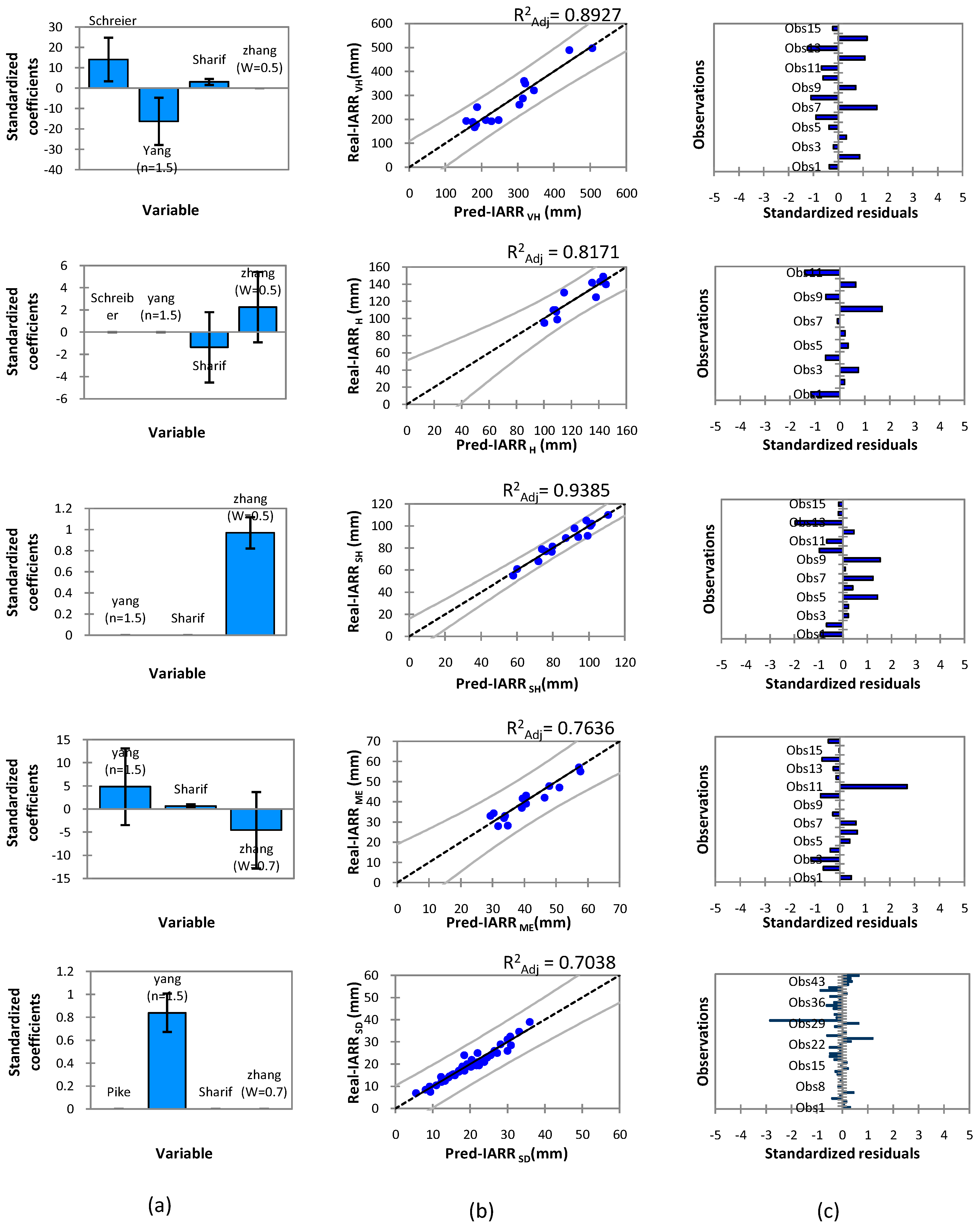
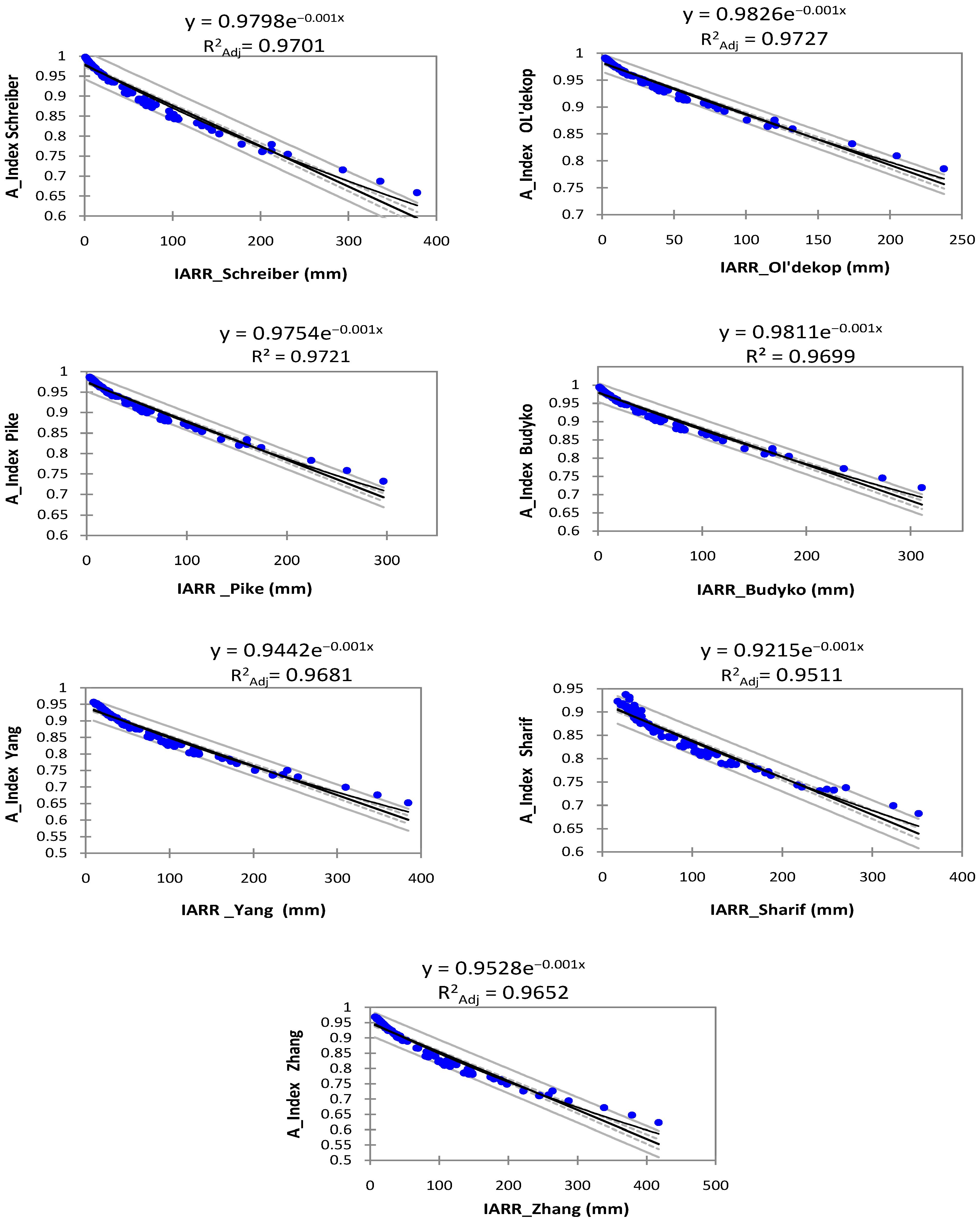
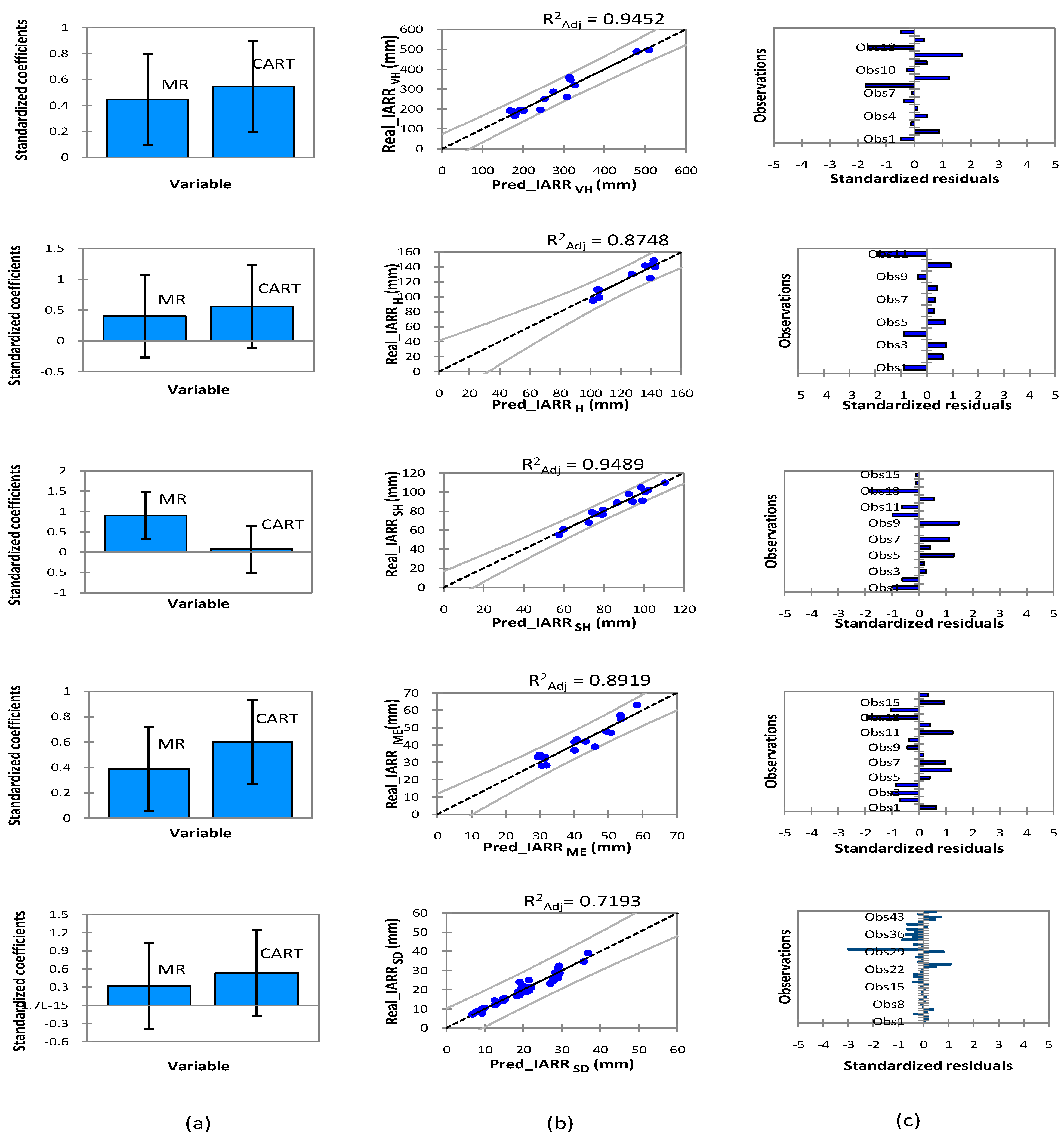
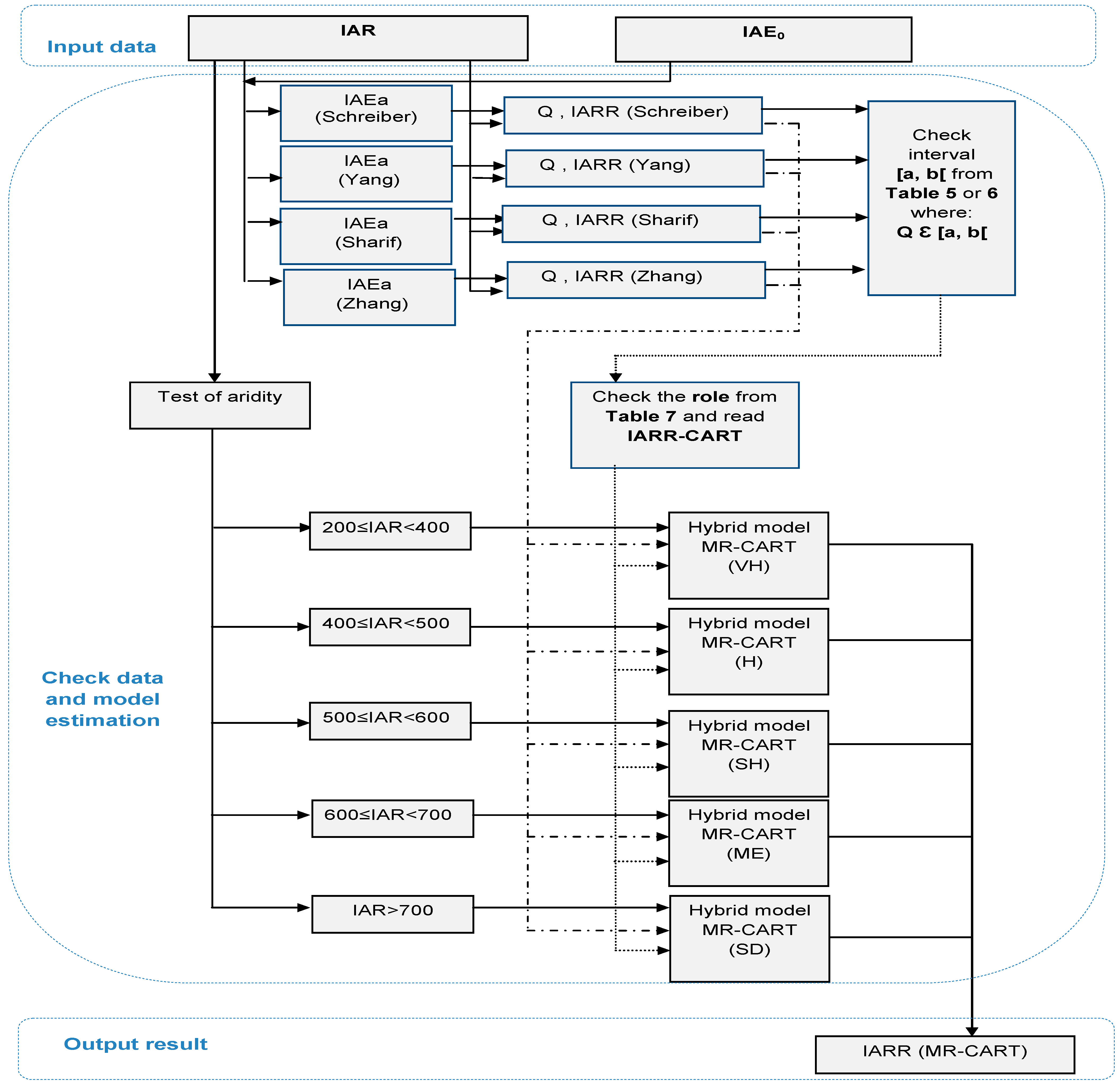
3.2. Experimental Results
Proposed Method
4. Discussion
5. Conclusions and Future Work
Author Contributions
Funding
Institutional Review Board Statement
Informed Consent Statement
Data Availability Statement
Acknowledgments
Conflicts of Interest
References
- Moran-Tejeda, E.; Ceballos-Barbancho, A.; Llorente-Pinto, J.M. Hydrological response of Mediterranean headwaters to climate oscillations and land-cover changes: The mountains of Duero River basin (Central Spain). Glob. Planet. Chang. 2010, 72, 39–49. [Google Scholar] [CrossRef]
- Shiklomanov, I.A. World Water Resources and Water Use: Present Assessment and Outlook for 2025; World Water Scenarios Analyses; Springer: Berlin/Heidelberg, Germany, 2000; p. 396. [Google Scholar]
- Vorosmarty, C.J.; Green, P.; Salisbury, J.; Lammers, R.B. Global water resources: Vulnerability from climate change and population growth. Science 2000, 289, 284–288. [Google Scholar] [CrossRef] [PubMed] [Green Version]
- Budyko, M.I. Climate and Life; Academic Press: Cambridge, MA, USA, 1974. [Google Scholar]
- Loumagne, C.; Chkir, N.; Normand, M.; OttlÉ, C.; Vidal-Madjar, D. Introduction of the soil/vegetation/atmosphere continuum in a conceptual rainfall/runoff model. Hydrol. Sci. J. 2009, 41, 889–902. [Google Scholar] [CrossRef]
- Sitterson, J.; Knightes, C.; Parmar, R.; Wolfe, K.; Avant, B.; Muche, M. An overview of rainfall-runoff model types. In Proceedings of the International Congress on Environmental Modelling and Software, Fort Collins, CO, USA, 27 June 2018. [Google Scholar]
- Rajurkar, M.P.; Kothyari, U.C.; Chaube, U.C. Modeling of the daily rainfall-runoff relationship with artificial neural network. J. Hydrol. 2004, 285, 96–113. [Google Scholar] [CrossRef]
- Schreiber, P. Über die Beziehungen zwischen dem Niederschlag und der Wasserführung der Flüsse in Mitteleuropa. Z. Meteorol. 1904, 21, 441–452. [Google Scholar]
- Ol’Dekop, E. Ob Isparenii s Poverkhnosti Rechnykh Baseeinov (On Evaporation from the Surface of River Basins); Trans. Meteorol. Observ. Lur-evskogo; University of Tartu: Tartu, Estonia, 1911; Volume 4. [Google Scholar]
- Budyko, M. Evaporation under Natural Conditions, Gidrometeorizdat, Leningrad; U.S. Department of Commerce : Washington, DC, USA, 1948; p. 635.
- Gentine, P.; D’Odorico, P.; Lintner, B.R.; Sivandran, G.; Salvucci, G. Interdependence of climate, soil, and vegetation as constrained by the Budyko curve. Geophys. Res. Lett. 2012, 39, L19404. [Google Scholar] [CrossRef] [Green Version]
- Sharif, H.O.; Crow, W.; Miller, N.L.; Wood, E.F. Multidecadal High-Resolution Hydrologic Modeling of the Arkansas–Red River Basin. J. Hydrometeorol. 2007, 8, 1111–1127. [Google Scholar] [CrossRef]
- Yang, H.; Yang, D.; Lei, Z.; Sun, F. New analytical derivation of the mean annual water-energy balance equation. Water Resour. Res. 2008, 44, W03410. [Google Scholar] [CrossRef]
- Guezgouz, N.; Boutoutaou, D.; Zeggane, H.; Chefrour, A. Multivariate statistical analysis of the groundwater flow in shallow aquifers: A case of the basins of northern Algeria. Arab. J. Geosci. 2017, 10, 1–8. [Google Scholar] [CrossRef]
- Zhang, L.; Dawes, W.R.; Walker, G.R. Response of mean annual evapotranspiration to vegetation changes at catchment scale. Water Resour. Res. 2001, 37, 701–708. [Google Scholar] [CrossRef]
- Turc, L. Calcul Du Bilan De L’eau Évaluation En Fonction Des Précipitations Et Des Températures; IAHS Publication: Wallingford, UK, 1954; Volume 37, pp. 88–200. [Google Scholar]
- Pike, J.G. The estimation of annual run-off from meteorological data in a tropical climate. J. Hydrol. 1964, 2, 116–123. [Google Scholar] [CrossRef]
- Shan, X.; Li, X.; Yang, H. Towards understanding the mean annual water-energy balance equation based on an ohms-type approach. Hydrol. Earth Syst. Sci. 2019, 1–17. [Google Scholar] [CrossRef]
- Budyko, M. The Heat Balance of the Earth’s Surface, US Dept. of Commerce; Weather Bureau: Washington, DC, USA, 1958.
- Brown, S.H. Multiple linear regression analysis: A matrix approach with MATLAB. Ala. J. Math. 2009, 34, 1–3. [Google Scholar]
- Adamowski, J.; Chan, H.F.; Prasher, S.O.; Ozga-Zielinski, B.; Sliusarieva, A. Comparison of multiple linear and nonlinear regression, autoregressive integrated moving average, artificial neural network, and wavelet artificial neural network methods for urban water demand forecasting in Montreal, Canada. Water Resour. Res. 2012, 48, 1–14. [Google Scholar] [CrossRef]
- Park, Y.W.; Klabjan, D. Subset selection for multiple linear regression via optimization. J. Global Optim. 2020, 77, 543–574. [Google Scholar] [CrossRef] [Green Version]
- Bevilacqua, M.; Braglia, M.; Montanari, R. The classification and regression tree approach to pump failure rate analysis. Reliab. Eng. Syst. Saf. 2003, 79, 59–67. [Google Scholar] [CrossRef]
- Kim, K.N.; Kim, D.W.; Jeong, M.A. The usefulness of a classification and regression tree algorithm for detecting perioperative transfusion-related pulmonary complications. Transfusion 2015, 55, 2582–2589. [Google Scholar] [CrossRef] [PubMed]
- Koon, S.; Petscher, Y. Comparing Methodologies for Developing an Early Warning System: Classification and Regression Tree Model versus Logistic Regression; REL 2015-077; Regional Educational Laboratory Southeast: Tallahassee, FL, USA, 2015. [Google Scholar]
- Chipman, H.A.; George, E.I.; McCulloch, R.E. Bayesian CART model search. J. Am. Stat. Assoc. 1998, 93, 935–948. [Google Scholar] [CrossRef]
- Machuca, C.; Vettore, M.V.; Krasuska, M.; Baker, S.R.; Robinson, P.G. Using classification and regression tree modelling to investigate response shift patterns in dentine hypersensitivity. BMC Med. Res. Methodol. 2017, 17, 120. [Google Scholar] [CrossRef] [Green Version]
- Patriche, C.V.; Radu, G.P.; Bogdan, R. Comparing linear regression and regression trees for spatial modelling of soil reaction in Dobrovăţ Basin (Eastern Romania). Bull. UASVM Agric. 2011, 68, 264–271. [Google Scholar] [CrossRef]
- Wilkinson, L. Tree structured data analysis: AID, CHAID and CART. Retrieved Febr. 1992, 1, 2008. [Google Scholar]
- Legates, D.R.; McCabe, G.J., Jr. Evaluating the use of “goodness-of-fit” measures in hydrologic and hydroclimatic model validation. Water Resour. Res. 1999, 35, 233–241. [Google Scholar] [CrossRef]
- Rosa, D.P.; Cantú-Lozano, D.; Luna-Solano, G.; Polachini, T.C.; Telis-Romero, J. Mathematical Modeling of Orange Seed Drying Kinetics. Ciência e Agrotecnologia 2015, 393, 291–300. [Google Scholar] [CrossRef] [Green Version]
- Chai, T.; Draxler, R.R. Root mean square error (RMSE) or mean absolute error (MAE)?–Arguments against avoiding RMSE in the literature. Geosci. Model Dev. 2014, 7, 1247–1250. [Google Scholar] [CrossRef] [Green Version]
- Hsu, H.; Lachenbruch, P.A. Paired t test. Wiley StatsRef: Stat. Ref. Online 2014, 7, 1247–1250. [Google Scholar] [CrossRef] [Green Version]
- Liang, J.; Pan, W.S. Testing The mean for business data: Should one use the z-test, t-test, f-test, the chi-square test, or the p-value method? J. Coll. Teach. Learn. (TLC) 2006, 3, 79–88. [Google Scholar] [CrossRef] [Green Version]
- Blackwell, M. Multiple Hypothesis Testing: The F-Test. Matt Blackwell Research. 2008, pp. 1–7. Available online: https://mattblackwell.org/files/teaching/ftests.pdf (accessed on 1 April 2022).
- Hodges, J.L. A bivariate sign test. Ann. Math. Stat. 1955, 26, 523–527. [Google Scholar] [CrossRef]
- Woolson, R.F. Wilcoxon signed-rank test. In Wiley Encyclopedia of Clinical Trials; D’Agostino, R.B., Sullivan, L., Massaro, J., Eds.; John Wiley & Sons, Inc.: Hoboken, NJ, USA, 2008. [Google Scholar] [CrossRef]


| Statistic | All Data | Very Humid | Humid | Semi-Humid | Mediterranean | Semi-Dry | ||||||||||||
|---|---|---|---|---|---|---|---|---|---|---|---|---|---|---|---|---|---|---|
| IARR | IAEo | IAR | IARR | IAEo | IAR | IARR | IAEo | IAR | IARR | IAEo | IAR | IARR | IAEo | IAR | IARR | IAEo | IAR | |
| N. data | 102.000 | 102.000 | 102.000 | 15.000 | 15.000 | 15.000 | 11.000 | 11.000 | 11.000 | 15.000 | 15.000 | 15.000 | 16.000 | 16.000 | 16.000 | 45.000 | 45.000 | 45.000 |
| Min | 7.000 | 1180.000 | 222.000 | 166.000 | 1190.000 | 700.000 | 95.000 | 1185.000 | 610.000 | 55.000 | 1180.000 | 501.000 | 28.000 | 1195.000 | 400.000 | 7.000 | 1210.000 | 222.000 |
| Max | 497.000 | 1610.000 | 1107.000 | 497.000 | 1455.000 | 1107.000 | 149.000 | 1445.000 | 695.000 | 110.000 | 1460.000 | 598.000 | 62.950 | 1445.000 | 483.000 | 51.000 | 1610.000 | 394.000 |
| Sum | 8335.362 | 137,863.000 | 50,455.600 | 4118.860 | 19,551.000 | 13,117.000 | 1351.291 | 14,573.000 | 7187.000 | 1283.000 | 19,605.000 | 8367.000 | 661.055 | 21,127.000 | 6888.000 | 921.156 | 63,007.000 | 14,896.600 |
| 1st Q | 20.625 | 1285.000 | 332.750 | 191.500 | 1237.500 | 783.500 | 109.000 | 1266.500 | 636.500 | 76.750 | 1222.000 | 535.500 | 33.022 | 1271.250 | 410.000 | 15.000 | 1350.000 | 309.000 |
| Median | 39.000 | 1357.500 | 415.500 | 250.000 | 1300.000 | 845.000 | 125.000 | 1340.000 | 650.000 | 89.000 | 1297.000 | 565.000 | 40.343 | 1345.000 | 425.500 | 19.500 | 1400.000 | 330.000 |
| 3rd Q | 104.250 | 1410.000 | 607.000 | 334.500 | 1353.500 | 951.500 | 141.000 | 1407.500 | 669.500 | 99.000 | 1392.000 | 582.500 | 47.197 | 1366.750 | 442.750 | 24.000 | 1450.000 | 351.000 |
| AV * | 252.000 | 1395.000 | 664.500 | 331.500 | 1322.500 | 903.500 | 122.000 | 1315.000 | 652.500 | 82.500 | 1320.000 | 549.500 | 45.475 | 1320.000 | 441.500 | 29.000 | 1410.000 | 308.000 |
| Mean | 81.719 | 1351.598 | 494.663 | 274.591 | 1303.400 | 874.467 | 122.845 | 1324.818 | 653.364 | 85.533 | 1307.000 | 557.800 | 41.316 | 1320.438 | 430.500 | 20.470 | 1400.156 | 331.036 |
| SD | 96.510 | 98.801 | 200.100 | 105.200 | 72.300 | 119.700 | 18.400 | 85.400 | 24.200 | 15.800 | 91.700 | 31.900 | 10.100 | 76.800 | 26.700 | 8.300 | 96.900 | 37.400 |
| CV ** | 1.181 | 0.073 | 0.404 | 0.383 | 0.055 | 0.137 | 0.1500 | 0.064 | 0.037 | 0.185 | 0.070 | 0.057 | 0.245 | 0.058 | 0.062 | 0.405 | 0.069 | 0.113 |
| Climate Floor | Statistic | Zhang W = 0.5 | Zhang W = 0.7 | Zhang W = 1.7 | Zhang W = 1.9 | Zhang W = 2.1 | Zhang W = 2.3 | Zhang W = 2.5 |
|---|---|---|---|---|---|---|---|---|
| Very humid | R2 | 0.685 | 0.685 | 0.677 | 0.675 | 0.673 | 0.671 | 0.668 |
| R2Adj | 0.661 | 0.66 | 0.653 | 0.65 | 0.648 | 0.646 | 0.643 | |
| MAE | 45.688 | 67.002 | 146.652 | 137.439 | 145.245 | 152.412 | 158.804 | |
| RMSE | 65.489 | 80.273 | 157.022 | 147.515 | 161.08 | 168.074 | 174.361 | |
| Humid | R2 | 0.803 | 0.801 | 0.808 | 0.809 | 0.809 | 0.81 | 0.81 |
| R2Adj | 0.792 | 0.777 | 0.787 | 0.787 | 0.788 | 0.788 | 0.789 | |
| MAE | 8.981 | 11.626 | 65.846 | 60.875 | 66.243 | 69.955 | 73.211 | |
| RMSE | 10.757 | 14.576 | 66.442 | 61.442 | 67.286 | 70.997 | 74.255 | |
| Semi-humid | R2 | 0.969 | 0.969 | 0.968 | 0.968 | 0.968 | 0.967 | 0.967 |
| R2Adj | 0.967 | 0.966 | 0.965 | 0.965 | 0.965 | 0.965 | 0.965 | |
| MAE | 7.017 | 7.172 | 44.687 | 41.146 | 47.407 | 50.014 | 52.287 | |
| RMSE | 8.066 | 8.51 | 45.413 | 41.831 | 48.277 | 50.91 | 53.208 | |
| Mediterranean | R2 | 0.48 | 0.525 | 0.446 | 0.445 | 0.445 | 0.444 | 0.444 |
| R2Adj | 0.441 | 0.516 | 0.407 | 0.406 | 0.405 | 0.404 | 0.404 | |
| MAE | 9.985 | 5.74 | 21.662 | 19.809 | 23.067 | 24.4 | 25.551 | |
| RMSE | 10.956 | 7.519 | 21.938 | 20.066 | 24.549 | 25.836 | 26.952 | |
| Semi-arid | R2 | 0.703 | 0.703 | 0.702 | 0.702 | 0.702 | 0.702 | 0.702 |
| R2Adj | 0.696 | 0.696 | 0.695 | 0.695 | 0.695 | 0.695 | 0.695 | |
| MAE | 4.706 | 2.202 | 9.733 | 8.853 | 12.352 | 12.974 | 13.507 | |
| RMSE | 5.875 | 4.764 | 10.27 | 9.346 | 13.83 | 14.449 | 14.982 |
| Climate Floor | Statistic | Yang n = 0.5 | Yang n = 1 | Yang n = 1.5 | Yang n = 2 | Yang n = 2.5 | Yang n = 3 | Yang n = 3.5 |
|---|---|---|---|---|---|---|---|---|
| Very humid | R2 | 0.669 | 0.684 | 0.690 | 0.692 | 0.691 | 0.689 | 0.685 |
| R2Adj | 0.643 | 0.659 | 0.666 | 0.668 | 0.668 | 0.665 | 0.661 | |
| MAE | 336.917 | 79.873 | 63.289 | 123.699 | 164.240 | 193.151 | 212.914 | |
| RMSE | 342.734 | 99.480 | 77.753 | 136.170 | 177.727 | 205.967 | 225.710 | |
| Humid | R2 | 0.509 | 0.731 | 0.792 | 0.810 | 0.815 | 0.815 | 0.814 |
| R2Adj | 0.455 | 0.701 | 0.769 | 0.789 | 0.794 | 0.795 | 0.794 | |
| MAE | 305.252 | 93.448 | 8.684 | 54.747 | 82.216 | 98.011 | 107.386 | |
| RMSE | 305.594 | 93.932 | 10.331 | 55.752 | 83.115 | 98.962 | 108.415 | |
| Semi-humid | R2 | 0.794 | 0.917 | 0.938 | 0.935 | 0.927 | 0.918 | 0.908 |
| R2Adj | 0.778 | 0.910 | 0.934 | 0.930 | 0.922 | 0.912 | 0.901 | |
| MAE | 268.481 | 81.956 | 4.148 | 39.989 | 60.321 | 71.227 | 77.258 | |
| RMSE | 268.806 | 82.122 | 4.831 | 40.731 | 61.185 | 72.240 | 78.394 | |
| Mediterranean | R2 | 0.466 | 0.497 | 0.513 | 0.442 | 0.425 | 0.413 | 0.404 |
| R2Adj | 0.428 | 0.462 | 0.508 | 0.402 | 0.384 | 0.371 | 0.362 | |
| MAE | 214.877 | 64.780 | 7.725 | 19.890 | 31.122 | 36.339 | 38.835 | |
| RMSE | 215.295 | 65.264 | 9.080 | 21.497 | 32.363 | 37.527 | 40.020 | |
| Semi-dry | R2 | 0.673 | 0.700 | 0.704 | 0.701 | 0.696 | 0.689 | 0.680 |
| R2Adj | 0.665 | 0.693 | 0.697 | 0.694 | 0.689 | 0.681 | 0.673 | |
| MAE | 161.191 | 43.641 | 4.446 | 11.120 | 16.653 | 18.861 | 19.773 | |
| RMSE | 162.451 | 44.379 | 5.674 | 12.587 | 18.100 | 20.383 | 21.348 |
| Climate Floor | Statistic | Real Data | Schreiber | Ol’dekop | Pike | Budyko | Yang | Sharif | Zhang |
|---|---|---|---|---|---|---|---|---|---|
| Very humid | 1st Q | 191.500 | 142.853 | 79.234 | 108.015 | 111.792 | 172.325 | 177.104 | 189.116 |
| Median | 250.000 | 201.822 | 114.986 | 152.211 | 159.778 | 223.041 | 216.700 | 244.418 | |
| 3rd Q | 334.500 | 221.681 | 126.426 | 167.167 | 175.508 | 246.757 | 253.496 | 275.501 | |
| Mean | 274.591 | 202.740 | 117.382 | 154.542 | 161.413 | 226.406 | 222.811 | 248.345 | |
| R2 | 1.000 | 0.690 | 0.672 | 0.662 | 0.690 | 0.690 | 0.775 | 0.685 | |
| R2Adj | 1.000 | 0.667 | 0.662 | 0.660 | 0.666 | 0.666 | 0.757 | 0.661 | |
| MAE | 0.000 | 84.731 | 157.209 | 123.699 | 118.372 | 63.289 | 61.615 | 75.688 | |
| RMSE | 0.000 | 93.259 | 171.808 | 136.170 | 129.444 | 77.753 | 80.017 | 85.489 | |
| Humid | 1st Q | 109.000 | 84.061 | 42.118 | 59.222 | 58.285 | 106.793 | 120.299 | 116.514 |
| Median | 125.000 | 90.628 | 45.682 | 64.058 | 63.409 | 114.036 | 127.279 | 124.550 | |
| 3rd Q | 141.000 | 101.443 | 56.376 | 77.984 | 79.338 | 131.099 | 140.595 | 143.678 | |
| Mean | 122.845 | 96.914 | 48.879 | 68.097 | 68.215 | 118.159 | 129.668 | 129.222 | |
| R2 | 1.000 | 0.714 | 0.712 | 0.710 | 0.713 | 0.792 | 0.756 | 0.794 | |
| R2Adj | 1.000 | 0.693 | 0.691 | 0.689 | 0.693 | 0.769 | 0.729 | 0.772 | |
| MAE | 0.000 | 24.930 | 73.966 | 54.747 | 54.629 | 8.684 | 10.912 | 8.081 | |
| RMSE | 0.000 | 24.863 | 74.958 | 55.752 | 55.488 | 10.331 | 12.595 | 10.057 | |
| Semi-humid | 1st Q | 76.750 | 46.232 | 27.957 | 39.717 | 37.178 | 76.460 | 90.785 | 80.750 |
| Median | 89.000 | 73.893 | 32.040 | 45.516 | 43.077 | 86.578 | 101.400 | 91.933 | |
| 3rd Q | 99.000 | 86.040 | 37.764 | 53.127 | 52.107 | 96.049 | 108.303 | 102.767 | |
| Mean | 85.533 | 74.706 | 32.188 | 45.544 | 43.579 | 85.132 | 98.614 | 92.477 | |
| R2 | 1.000 | 0.928 | 0.934 | 0.935 | 0.930 | 0.935 | 0.927 | 0.939 | |
| R2Adj | 1.000 | 0.922 | 0.929 | 0.930 | 0.925 | 0.930 | 0.921 | 0.933 | |
| MAE | 0.000 | 14.828 | 53.345 | 40.989 | 41.954 | 4.148 | 13.081 | 3.017 | |
| RMSE | 0.000 | 14.199 | 54.232 | 40.731 | 42.519 | 5.831 | 14.285 | 4.066 | |
| Mediterranean | 1st Q | 33.022 | 16.436 | 12.819 | 18.638 | 14.631 | 41.936 | 36.491 | 36.150 |
| Median | 40.343 | 19.794 | 14.250 | 20.648 | 16.972 | 45.478 | 52.701 | 39.429 | |
| 3rd Q | 47.197 | 21.590 | 15.535 | 22.503 | 18.518 | 48.959 | 62.517 | 42.789 | |
| Mean | 41.316 | 20.432 | 14.798 | 21.426 | 17.626 | 46.576 | 50.516 | 40.699 | |
| R2 | 1.000 | 0.407 | 0.440 | 0.442 | 0.418 | 0.616 | 0.697 | 0.612 | |
| R2Adj | 1.000 | 0.364 | 0.400 | 0.402 | 0.377 | 0.608 | 0.675 | 0.603 | |
| MAE | 0.000 | 20.884 | 26.518 | 19.890 | 23.690 | 7.725 | 11.118 | 5.740 | |
| RMSE | 0.000 | 22.330 | 27.882 | 21.497 | 25.060 | 9.080 | 12.769 | 7.519 | |
| Semi-dry | 1st Q | 15.000 | 3.064 | 4.741 | 6.999 | 3.904 | 19.140 | 25.135 | 15.032 |
| Median | 19.500 | 5.274 | 6.282 | 9.241 | 5.778 | 23.808 | 28.588 | 19.284 | |
| 3rd Q | 24.000 | 7.708 | 7.839 | 11.504 | 7.638 | 28.714 | 36.772 | 23.622 | |
| Mean | 20.470 | 5.641 | 6.366 | 9.350 | 6.004 | 23.856 | 28.543 | 19.376 | |
| R2 | 1.000 | 0.679 | 0.701 | 0.701 | 0.690 | 0.706 | 0.701 | 0.703 | |
| R2Adj | 1.000 | 0.671 | 0.694 | 0.694 | 0.683 | 0.700 | 0.694 | 0.696 | |
| MAE | 0.000 | 14.830 | 14.104 | 13.120 | 14.466 | 4.446 | 11.481 | 5.202 | |
| RMSE | 0.000 | 15.959 | 15.566 | 14.587 | 15.748 | 5.674 | 12.775 | 6.764 |
| Climate Floor | p-Value | Objects | % | Parent Node | Sons Node | W.B.M * | IARR (W.B.M) | A-Index ** | Q *** |
|---|---|---|---|---|---|---|---|---|---|
| Very humid | 0 | 15 | 100.00% | ||||||
| 0 | 6 | 40.00% | 1 | 2 | Zhang (W = 0.5) | [141.207, 209.585] | [0.772, 0.827] | [772.652, 827.330] | |
| 0 | 5 | 33.33% | 1 | 3 | Zhang (W = 0.5) | [209.585, 275.501] | [0.723, 0.772] | [723.360, 772.652] | |
| 0.031 | 4 | 26.67% | 1 | 4 | Zhang (W = 0.5) | [275.501, 417.300] | [0.627, 0.723] | [627.731, 723.360] | |
| 0 | 2 | 13.33% | 4 | 5 | Sharif | [249.605, 296.940] | [0.684, 0.717] | [684.763, 717.950] | |
| 0 | 2 | 13.33% | 4 | 6 | Sharif | [296.940, 351.434] | [0.648, 0.684] | [648.441, 684.763] | |
| 0.0225 | 11 | 100.00% | |||||||
| 0.0033 | 7 | 63.64% | 1 | 2 | Schreiber | [67.956, 98.557] | [0.835, 0.860] | [835.011, 860.960] | |
| Humid | 0 | 4 | 36.36% | 1 | 3 | Schreiber | [98.557, 106.253] | [0.828, 0.835] | [828.610, 835.011] |
| 0 | 5 | 45.45% | 2 | 4 | Yang (n = 1.5) | [102.302, 111.657] | [0.844, 0.852] | [844.450, 852.380] | |
| 0 | 2 | 18.18% | 2 | 5 | Yang (n = 1.5) | [111.657, 123.606] | [0.834, 0.844] | [834.420, 844.450] | |
| Semi-humid | 0 | 15 | 100.00% | ||||||
| 0 | 2 | 13.33% | 1 | 2 | Schreiber | [32.268, 38.265] | [0.943, 0.948] | [943.020, 948.690] | |
| 0 | 6 | 40.00% | 1 | 3 | Schreiber | [38.265, 57.529] | [0.925, 0.943] | [925.021, 943.020] | |
| 0 | 5 | 33.33% | 1 | 4 | Schreiber | [57.529, 68.321] | [0.915, 0.925] | [915.091, 925.021] | |
| 0 | 2 | 13.33% | 1 | 5 | Schreiber | [68.321, 76.457] | [0.907, 0.915] | [907.670, 915.091] |
| Climate Floor | p-Value | Objects | % | Parent Node | Sons Node | W.B.M * | IARR (W.B.M) | A-Index ** | Q *** |
|---|---|---|---|---|---|---|---|---|---|
| Mediterranean | 0.0371 | 16 | 100.00% | ||||||
| 0 | 11 | 68.75% | 1 | 2 | Zhang (W = 0.7) | [31.604, 42.121] | [0.913, 0.923 ] | [913.504, 923.161] | |
| 0 | 5 | 31.25% | 1 | 3 | Zhang (W = 0.7) | [42.121, 53.600] | [0.903, 0.913] | [903.070, 913.504] | |
| 0 | 6 | 37.50% | 2 | 4 | Sharif | [26.037, 47.666] | [0.878, 0.897] | [878.610, 897.822] | |
| 0 | 4 | 25.00% | 2 | 5 | Sharif | [47.666, 60.976] | [0.867, 0.878] | [867.011, 878.610] | |
| 0 | 1 | 6.25% | 2 | 6 | Sharif | [60.976, 61.917] | [0.866, 0.867] | [866.170, 867.011] | |
| Semi-dry | 0 | 45 | 100.00% | ||||||
| 0 | 2 | 4.44% | 1 | 2 | Sharif | [17.101, 21.332] | [0.902, 0.905] | [902.051, 905.882] | |
| 0 | 3 | 6.67% | 1 | 3 | Sharif | [21.332, 25.534] | [0.898, 0.902] | [898.270, 902.051] | |
| 0 | 3 | 6.67% | 1 | 4 | Sharif | [25.534, 28.247] | [0.895, 0.898] | [895.831, 898.270] | |
| 0 | 5 | 11.11% | 1 | 5 | Sharif | [28.247, 31.418] | [0.893, 0.895] | [893.000, 895.831] | |
| 0 | 10 | 22.22% | 1 | 6 | Sharif | [31.418, 35.862] | [0.889, 0.893] | [889.041, 893.000] | |
| 0 | 9 | 20.00% | 1 | 7 | Sharif | [35.862, 39.475] | [0.885, 0.889] | [885.833, 889.041] | |
| 0 | 11 | 24.44% | 1 | 8 | Sharif | [39.475, 48.371] | [0.877, 0.885] | [877.990, 885.833] | |
| 0 | 2 | 4.44% | 1 | 9 | Sharif | [48.371, 52.023] | [0.874, 0.877] | [874.791, 877.990] |
| Climate Floor | Node Son | Condition | IARR-CART |
|---|---|---|---|
| Very humid | Node2 | If Q 1 (Zhang) ∈ [772.652, 827.330] or IARR 2 (Zhang) ∈ [141.207, 209.585] | 185.00 |
| Node3 | If Q (Zhang) ∈ [723.360, 772.652] or IARR (Zhang) ∈ [209.585, 275.501] | 307.80 | |
| Node4 | If Q (Zhang) ∈ [627.731, 723.360] or IARR (Zhang) ∈ [275.501, 417.300] | 367.47 | |
| Node5 | If (Q (Sharif) ∈ [684.763, 717.950] and Q (Zhang) ∈ [627.731, 723.360]) or (IARF (Sharif) ∈ [249.605, 296.940] and IARR (Zhang) ∈ [275.501, 417.300]) | 241.93 | |
| Node6 | If(Q (Sharif) ∈ [648.441, 684.763] and Q (Zhang) ∈ [627.731, 723.360]) or (IARR (Sharif) ∈ [296.940, 351.434] and IARR (Zhang) ∈ [275.501, 417.300]) | 493.00 | |
| Humid | Node2 | IfQ (Schreiber) ∈ [835.011, 860.960] or IARR (Schreiber) ∈ [67.956, 98.557] | 113.47 |
| Node3 | If Q (Schreiber) ∈ [828.610, 835.011] or IARR (Schreiber) ∈ [98.557, 106.253] | 139.25 | |
| Node4 | If (Q (Yang) ∈ [844.450, 852.380] and Q (Schreiber) ∈ [835.011, 860.960]) or (IARR (Yang) ∈ [102.302, 111.657] and IARR (Schreiber) ∈ [67.956, 98.557]) | 104.40 | |
| Node5 | If (Q (Yang) ∈ [834.420, 844.450] and Q (Schreiber) ∈ [835.011, 860.960]) or (IARR (Yang) ∈ [111.657, 123.606] and IARR(Schreiber) ∈ [67.956, 98.557]) | 136.15 | |
| Semi-humid | Node2 | IfQ (Schreiber) ∈ [943.020, 948.690] or IARR (Schreiber) ∈ [32.268, 38.265] | 58.00 |
| Node3 | If Q (Schreiber) ∈ [925.021, 943.020] or IARR (Schreiber) ∈ [38.265, 57.529] | 78.50 | |
| Node4 | If Q (Schreiber) ∈ [915.091, 925.021] or IARR (Schreiber) ∈ [57.529, 68.321] | 96.80 | |
| Node5 | If Q (Schreiber) ∈ [907.670, 915.091] or IARR (Schreiber) ∈ [68.321, 76.457] | 106.00 | |
| Mediterranean | Node2 | If Q (Zhang) ∈ [913.504, 923.161] or IARR (Zhang) ∈ [31.604, 42.121] | 37.75 |
| Node3 | If Q (Zhang) ∈ [903.070, 913.504] or IARR (Zhang) ∈ [42.121, 53.600] | 49.16 | |
| Node4 | If (Q (Sharif) ∈ [878.610, 897.822] and Q(Zhang) ∈ [913.504, 923.161]) or (IARR (Sharif) ∈ [26.037, 47.666] and IARR (Zhang) ∈ [31.604, 42.121]) | 31.42 | |
| Node5 | If (Q (Sharif) ∈ [867.011, 878.610] and Q (Zhang) ∈ [913.504, 923.161]) or (IARR (Sharif) ∈ [47.666, 60.976] and IARR (Zhang) ∈ [31.604, 42.121]) | 40.95 | |
| Node6 | If (Q (Sharif) ∈ [866.170, 867.011] and Q (Zhang) ∈ [913.504, 923.161]) or (IARR (Sharif) ∈ [60.976, 61.917] and IARR (Zhang) ∈ [31.604, 42.121]) | 62.95 | |
| Semi-dry | Node2 | IfQ (Sharif) ∈ [902.051, 905.882] or IARR (Sharif) ∈ [17.101, 21.332] | 7.75 |
| Node3 | If Q (Sharif) ∈ [898.270, 902.051] or IARR (Sharif) ∈ [21.332, 25.534] | 9.33 | |
| Node4 | If Q (Sharif) ∈ [895.831, 898.270] or IARR (Sharif) ∈ [25.534, 28.247] | 12.94 | |
| Node5 | If Q (Sharif) ∈ [893.000, 895.831] or IARR (Sharif) ∈ [28.247, 31.418] | 14.82 | |
| Node6 | If Q (Sharif) ∈ [889.041, 893.000] or IARR (Sharif) ∈ [31.418, 35.862] | 19.28 | |
| Node7 | If Q (Sharif) ∈ [885.833, 889.041] or IARR (Sharif) ∈ [35.862, 39.475] | 20.87 | |
| Node8 | If Q (Sharif) ∈ [877.990, 885.833] or IARR (Sharif) ∈ [39.475, 48.371] | 28.22 | |
| Node9 | If Q (Sharif) ∈ [874.791, 877.990] or IARR (Sharif) ∈ [48.371, 52.023] | 36.84 |
| Climate Floor | Parameters | Real Data | MR Model | CART Model | (MR-CART) Model |
|---|---|---|---|---|---|
| Very humid | Min | 166.000 | 157.291 | 185.000 | 167.580 |
| Max | 497.000 | 505.874 | 493.000 | 509.539 | |
| Mean | 274.591 | 274.512 | 274.591 | 274.550 | |
| SD | 105.244 | 99.371 | 100.403 | 102.307 | |
| R2 | 1.000 | 0.899 | 0.922 | 0.957 | |
| R2Adj | 1.000 | 0.893 | 0.910 | 0.945 | |
| RMSE | 0.000 | 40.254 | 33.891 | 27.537 | |
| MAE | 0.000 | 28.083 | 23.644 | 19.211 | |
| Humid | Min | 95.000 | 100.494 | 104.400 | 98.252 |
| Max | 149.000 | 145.499 | 139.250 | 148.168 | |
| Mean | 122.845 | 123.107 | 122.845 | 118.843 | |
| SD | 18.355 | 16.629 | 16.872 | 17.628 | |
| R2 | 1.000 | 0.825 | 0.851 | 0.886 | |
| R2Adj | 1.000 | 0.817 | 0.845 | 0.875 | |
| RMSE | 0.000 | 9.204 | 7.990 | 7.614 | |
| MAE | 0.000 | 7.684 | 6.671 | 6.357 | |
| Semi-humid | Min | 55.000 | 57.891 | 58.000 | 57.662 |
| Max | 110.000 | 110.844 | 106.000 | 110.433 | |
| Mean | 85.533 | 85.620 | 85.533 | 85.506 | |
| SD | 15.770 | 15.290 | 14.800 | 15.469 | |
| R2 | 1.000 | 0.943 | 0.889 | 0.958 | |
| R2Adj | 1.000 | 0.939 | 0.881 | 0.949 | |
| RMSE | 0.000 | 4.199 | 5.849 | 4.049 | |
| MAE | 0.000 | 3.653 | 5.089 | 3.522 | |
| Mediterranean | Min | 28.000 | 29.279 | 31.421 | 29.463 |
| Max | 62.950 | 57.507 | 62.950 | 58.365 | |
| Mean | 41.316 | 41.229 | 41.316 | 41.310 | |
| SD | 10.083 | 8.793 | 9.231 | 9.521 | |
| R2 | 1.000 | 0.772 | 0.841 | 0.904 | |
| R2Adj | 1.000 | 0.764 | 0.838 | 0.892 | |
| RMSE | 0.000 | 5.661 | 4.336 | 3.678 | |
| MAE | 0.000 | 4.322 | 3.310 | 2.808 | |
| Semi-dry | Min | 7.000 | 5.524 | 7.750 | 6.952 |
| Max | 51.000 | 35.852 | 36.845 | 37.724 | |
| Mean | 20.470 | 20.401 | 20.470 | 21.026 | |
| SD | 8.349 | 6.984 | 7.153 | 7.271 | |
| R2 | 1.000 | 0.711 | 0.720 | 0.723 | |
| R2Adj | 1.000 | 0.704 | 0.714 | 0.719 | |
| RMSE | 0.000 | 4.648 | 4.570 | 4.521 | |
| MAE | 0.000 | 2.148 | 2.112 | 2.090 |
| Statistic | Real Data | Schreiber | Ol’dekop | Pike | Budyko | Yang | Sharif | Zhang | MR | CART | MR-CART |
|---|---|---|---|---|---|---|---|---|---|---|---|
| Min | 7.000 | 0.555 | 2.039 | 3.029 | 1.298 | 9.552 | 17.101 | 6.913 | 5.524 | 7.750 | 6.952 |
| Max | 497.00 | 377.825 | 237.453 | 296.477 | 310.726 | 384.671 | 351.434 | 417.300 | 505.874 | 493.000 | 502.539 |
| Mean | 20.625 | 5.981 | 6.771 | 9.950 | 6.331 | 25.252 | 35.629 | 20.618 | 21.852 | 20.867 | 20.844 |
| 1st Q | 39.000 | 18.680 | 13.995 | 20.294 | 16.404 | 44.170 | 50.550 | 38.715 | 37.485 | 38.896 | 38.924 |
| Median | 104.25 | 72.775 | 41.415 | 58.088 | 57.358 | 104.230 | 116.995 | 113.758 | 105.825 | 104.400 | 103.650 |
| 3rd Q | 81.719 | 52.926 | 32.396 | 44.254 | 42.916 | 76.388 | 84.857 | 78.989 | 81.704 | 81.719 | 81.716 |
| SD | 96.512 | 74.249 | 42.718 | 55.139 | 58.991 | 75.245 | 69.890 | 85.124 | 95.493 | 95.639 | 95.986 |
| T-test | 1.000 | <0.0001 | <0.0001 | <0.0001 | <0.0001 | 0.078 | 0.347 | 0.290 | 0.835 | 0.833 | 0.845 |
| Z-test | 1.000 | <0.0001 | <0.0001 | <0.0001 | <0.0001 | 0.075 | 0.345 | 0.287 | 0.830 | 0.828 | 0.844 |
| F-test | 1.000 | 0.009 | <0.0001 | <0.0001 | <0.0001 | 0.063 | 0.081 | 0.209 | 0.915 | 0.927 | 0.939 |
| Sign-test | 1.000 | <0.0001 | <0.0001 | <0.0001 | <0.0001 | 0.001 | <0.0001 | 0.421 | 0.773 | 0.326 | 0.773 |
| WSR-test | 1.000 | <0.0001 | <0.0001 | <0.0001 | <0.0001 | 0.032 | <0.0001 | 0.447 | 0.705 | 0.335 | 0.721 |
Publisher’s Note: MDPI stays neutral with regard to jurisdictional claims in published maps and institutional affiliations. |
© 2022 by the authors. Licensee MDPI, Basel, Switzerland. This article is an open access article distributed under the terms and conditions of the Creative Commons Attribution (CC BY) license (https://creativecommons.org/licenses/by/4.0/).
Share and Cite
Aieb, A.; Liotta, A.; Kadri, I.; Madani, K. A Hybrid Water Balance Machine Learning Model to Estimate Inter-Annual Rainfall-Runoff. Sensors 2022, 22, 3241. https://doi.org/10.3390/s22093241
Aieb A, Liotta A, Kadri I, Madani K. A Hybrid Water Balance Machine Learning Model to Estimate Inter-Annual Rainfall-Runoff. Sensors. 2022; 22(9):3241. https://doi.org/10.3390/s22093241
Chicago/Turabian StyleAieb, Amir, Antonio Liotta, Ismahen Kadri, and Khodir Madani. 2022. "A Hybrid Water Balance Machine Learning Model to Estimate Inter-Annual Rainfall-Runoff" Sensors 22, no. 9: 3241. https://doi.org/10.3390/s22093241