Author Contributions
Conceptualization, S.G., R.A.K. and R.T.; methodology, S.G., R.A.K. and R.T.; software, S.G., R.A.K. and R.T.; validation, S.G., R.A.K. and R.T.; formal analysis, S.G., R.A.K. and R.T.; investigation, S.G., R.A.K. and R.T.; resources, R.A.K.; data curation, S.G., R.A.K. and R.T.; writing—original draft preparation, S.G.; writing—review and editing, R.A.K.; visualization, S.G.; supervision, R.A.K.; project administration, R.A.K.; funding acquisition, R.A.K. All authors have read and agreed to the published version of the manuscript.
Figure 1.
Sample images from the PRIMAVERA dataset.
Figure 1.
Sample images from the PRIMAVERA dataset.
Figure 2.
Diagram of overall vehicle matching algorithm.
Figure 2.
Diagram of overall vehicle matching algorithm.
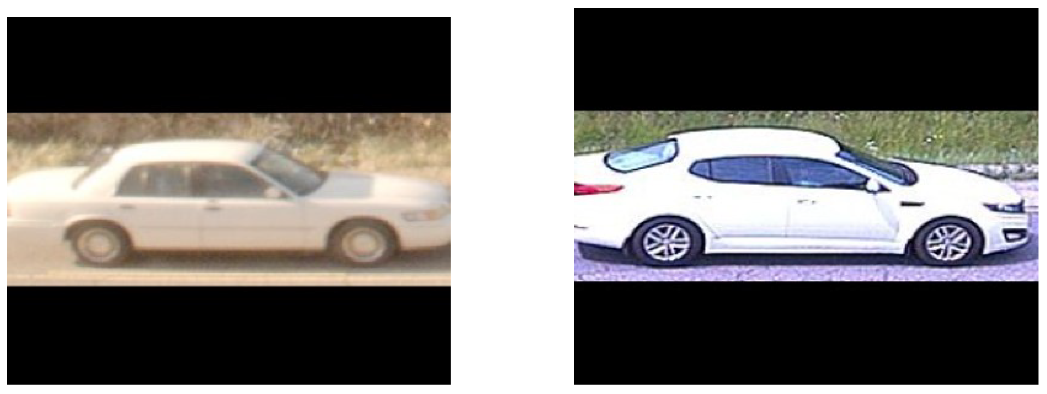
Figure 3.
Two vehicle images and their detected wheels.
Figure 3.
Two vehicle images and their detected wheels.
Figure 4.
Performance of whole-vehicle matching neural network during training.
Figure 4.
Performance of whole-vehicle matching neural network during training.
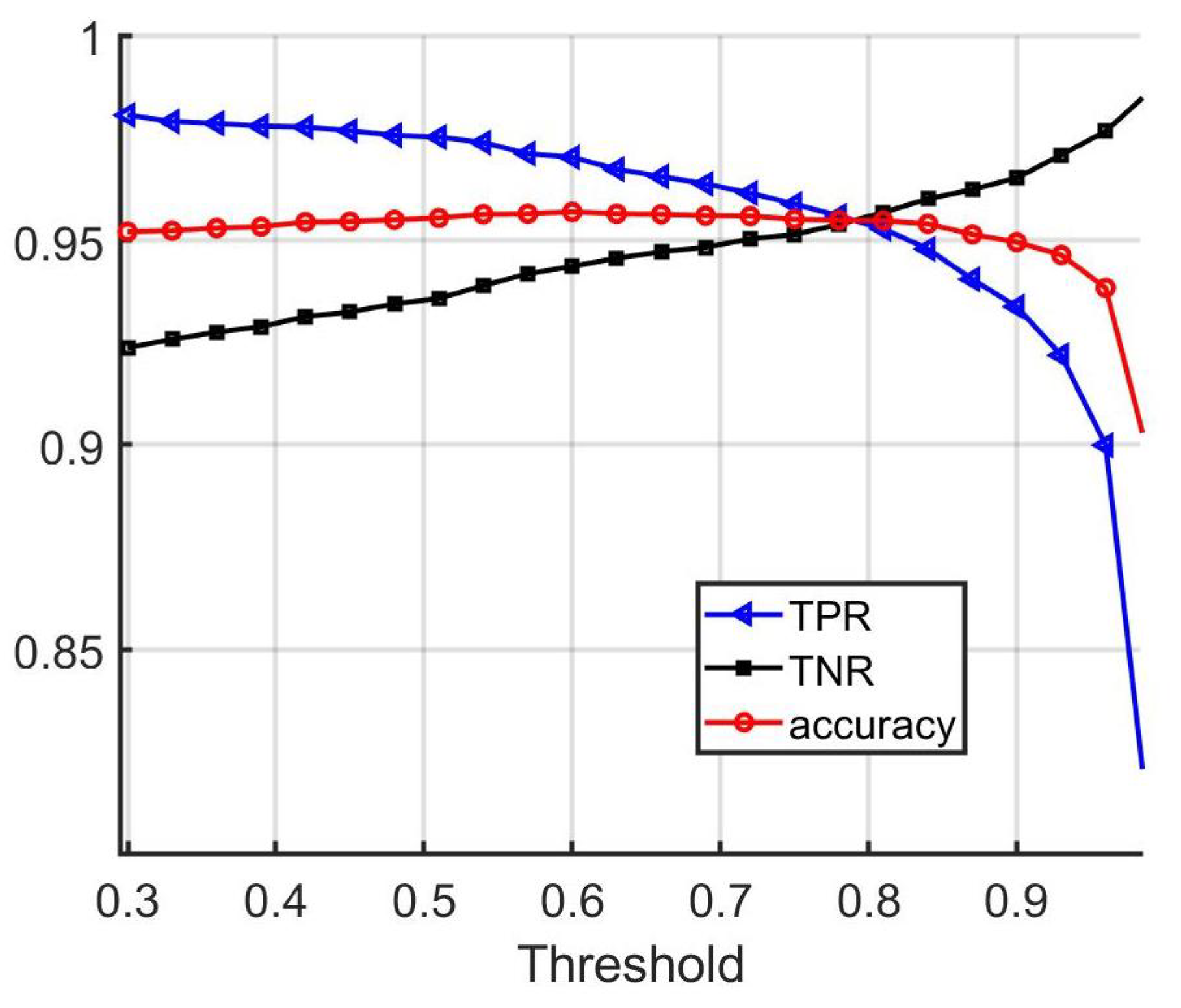
Figure 5.
Performance of the vehicle matching network on the validation set with different threshold values.
Figure 5.
Performance of the vehicle matching network on the validation set with different threshold values.
Figure 6.
Comparison of training set performance during training between wheel-locking and non-wheel-locking preprocessing approaches.
Figure 6.
Comparison of training set performance during training between wheel-locking and non-wheel-locking preprocessing approaches.
Figure 7.
Comparison of validation set performance during training between wheel-locking and non-wheel-locking preprocessing approaches.
Figure 7.
Comparison of validation set performance during training between wheel-locking and non-wheel-locking preprocessing approaches.
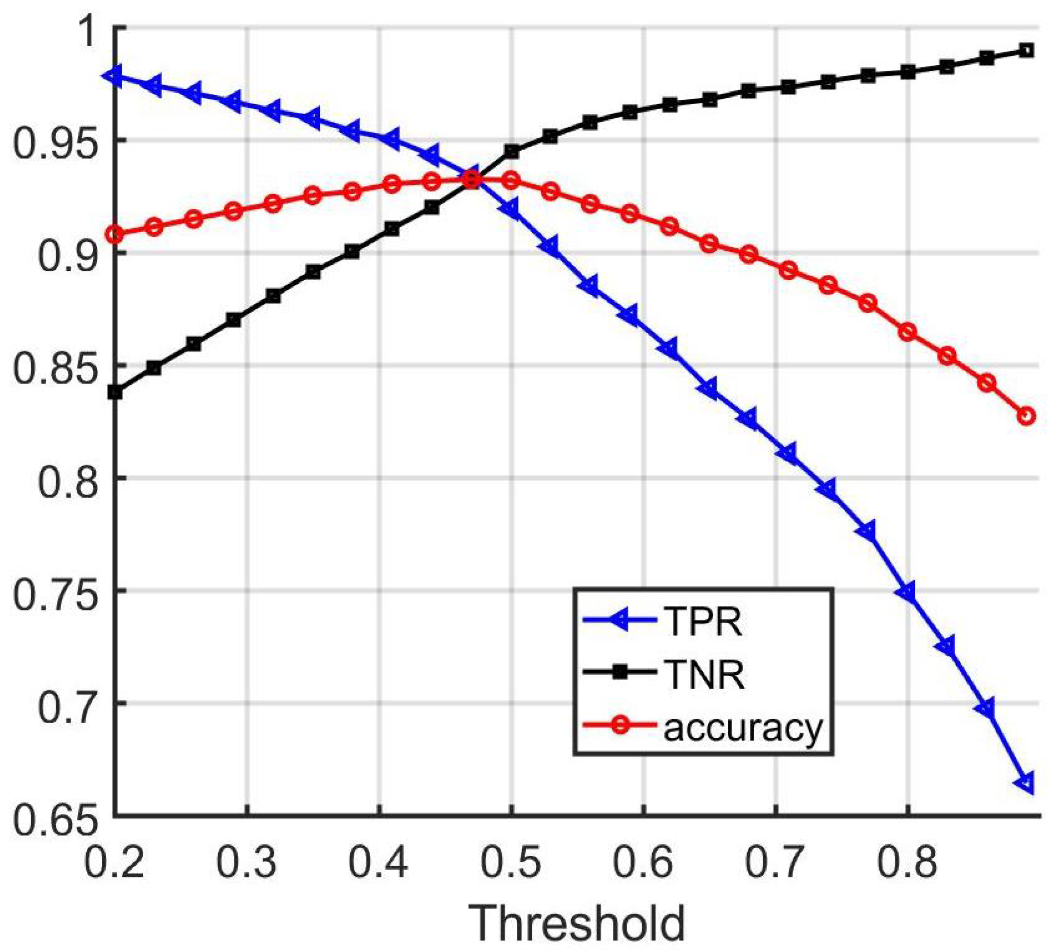
Figure 8.
Performance of wheel matching network.
Figure 8.
Performance of wheel matching network.
Figure 9.
Performance of decision fusion by averaging.
Figure 9.
Performance of decision fusion by averaging.
Figure 10.
ROC curves comparing the performances of whole-vehicle-only matching, wheels-only matching, and averaging-based decision fusion of the two matching approaches.
Figure 10.
ROC curves comparing the performances of whole-vehicle-only matching, wheels-only matching, and averaging-based decision fusion of the two matching approaches.
Figure 11.
Comparison of the baseline, vehicle, and wheel-network-matching accuracies.
Figure 11.
Comparison of the baseline, vehicle, and wheel-network-matching accuracies.
Figure 12.
Comparison of the baseline, vehicle, and wheel-network-matching true positive rates.
Figure 12.
Comparison of the baseline, vehicle, and wheel-network-matching true positive rates.
Figure 13.
Comparison of the baseline, vehicle, and wheel-network-matching true negative rates.
Figure 13.
Comparison of the baseline, vehicle, and wheel-network-matching true negative rates.
Figure 14.
Vehicle similarity score = 0.958; wheel similarity scores = 0.01, 0.001.
Figure 14.
Vehicle similarity score = 0.958; wheel similarity scores = 0.01, 0.001.
Figure 15.
Vehicle similarity score = 0.64; wheel similarity scores = 0.02, 0.01.
Figure 15.
Vehicle similarity score = 0.64; wheel similarity scores = 0.02, 0.01.
Figure 16.
Vehicle similarity score = 0.91; wheel similarity scores = 0.01, 0.03.
Figure 16.
Vehicle similarity score = 0.91; wheel similarity scores = 0.01, 0.03.
Figure 17.
Decision fusion network.
Figure 17.
Decision fusion network.
Figure 18.
Comparison of baseline, majority vote, soft vote, and fusion network matching accuracy.
Figure 18.
Comparison of baseline, majority vote, soft vote, and fusion network matching accuracy.
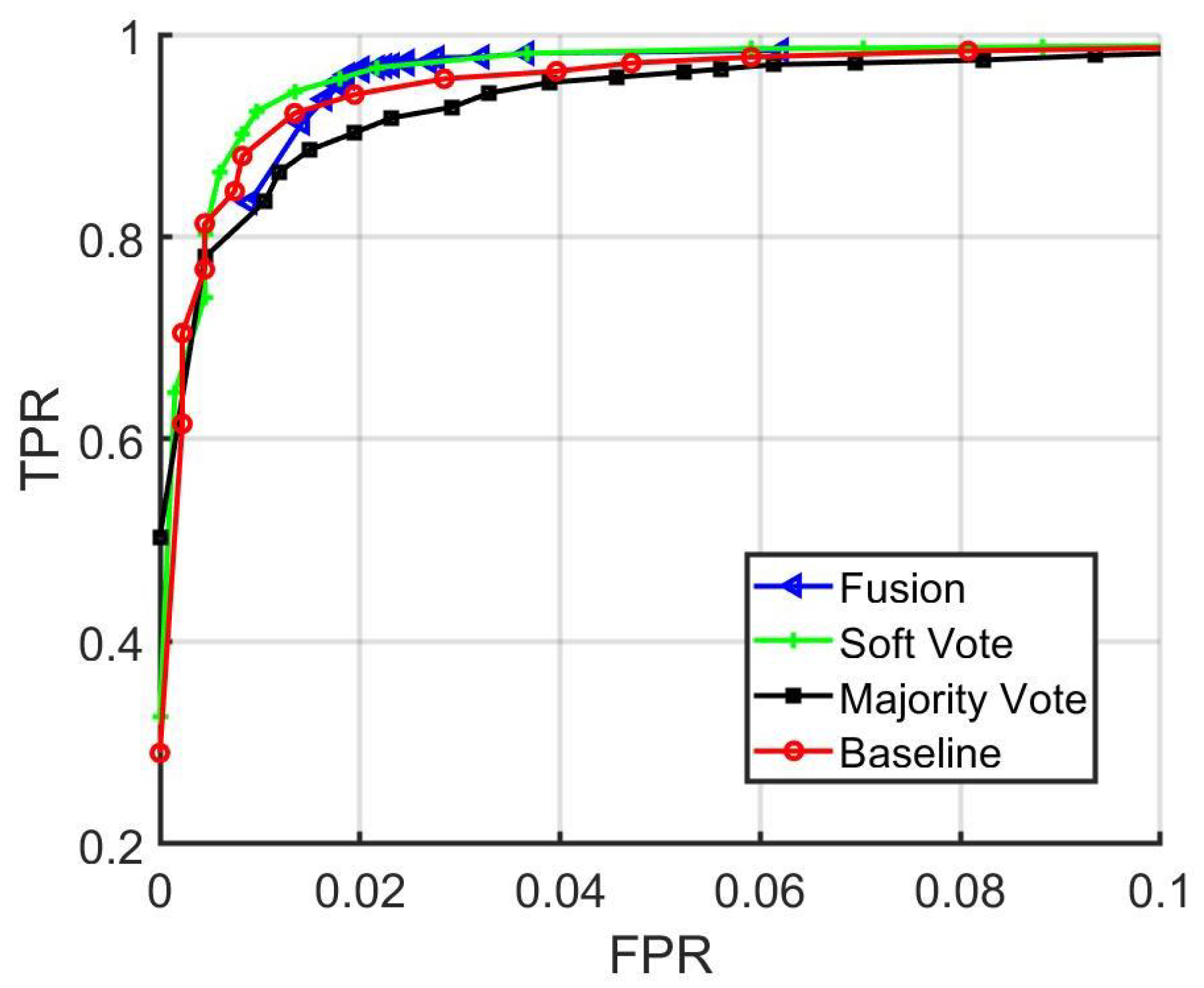
Figure 19.
Baseline, majority vote, soft vote, and fusion network ROC curves.
Figure 19.
Baseline, majority vote, soft vote, and fusion network ROC curves.
Table 1.
Vehicle matching network—each branch’s structure.
Table 1.
Vehicle matching network—each branch’s structure.
| Layer | Structure | Activation |
|---|
| Layer 1 | 4 × 3 × 3 | Relu |
| Layer 2 | 8 × 3 × 3 | Relu |
| Layer 3 | 16 × 3 × 3 | Relu |
| Layer 4 | 32 × 3 × 3 | Relu |
| Layer 5 | 32 × 3 × 3 | Relu |
| Layer 6 | 32 × 3 × 3 | Relu |
| Layer 7 | 32 × 3 × 3 | Relu |
Table 2.
Vehicle matching network—matching network structure.
Table 2.
Vehicle matching network—matching network structure.
| Layer | Structure | Activation |
|---|
| Layer 1 | 64 × 3 × 3 | Relu |
| Layer 2 | 64 × 3 × 3 | Relu |
| Layer 3 | 64 × 2 × 2 | Relu |
| Layer 4 | 64 × 1 × 1 | Relu |
| Layer 5 | 32 × 1 × 1 | Relu |
| Layer 6 | 1 × 1 × 1 | Relu |
Table 3.
Vehicle matching network performance.
Table 3.
Vehicle matching network performance.
| | Matching Accuracy |
|---|
| Training | 95.45% |
| Validation | 95.20% |
Table 4.
Wheel matching network structure.
Table 4.
Wheel matching network structure.
| Layer | Structure | Activation |
|---|
| Layer 1 | 64 × 10 × 10 | Relu |
| Layer 2 | 128 × 7 × 7 | Relu |
| Layer 3 | 128 × 4 × 4 | Relu |
| Layer 4 | 256 × 4 × 4 | Relu |
| Layer 5 | 4096 × 1 | Sigmoid |
Table 5.
Wheel matching network performance.
Table 5.
Wheel matching network performance.
| | Matching Accuracy |
|---|
| Training | 96.95% |
| Validation | 93.21% |
Table 6.
Average fusion network performance on test data.
Table 6.
Average fusion network performance on test data.
| | Matching Accuracy |
|---|
| Vehicle Matching Score | 95.5% |
| Wheel Matching Scores | 93.21% |
| Average | 97.63% |
Table 7.
Decision fusion network structure.
Table 7.
Decision fusion network structure.
| Layer | Structure | Activation |
|---|
| Layer 1 | 100 | Relu |
| Layer 2 | 70 | Relu |
| Layer 3 | 20 | Relu |
| Layer 4 | 1 | Sigmoid |
Table 8.
Comparison between fusion methods and no fusion on a portion of the testing data.
Table 8.
Comparison between fusion methods and no fusion on a portion of the testing data.
| | Fusion Network | Soft Voting | Baseline | Majority Voting | Vehicle Score | Wheel Scores |
|---|
| Accuracy | 97.77 ± 0.56% | 97.28 ± 0.62% | 96.31 ± 0.71% | 95.68 ± 0.77% | 95.46 ± 0.79% | 92.93 ± 0.97% |


