
Probabilistic 3D Reconstruction Using Two Sonar Devices


Abstract
:1. Introduction
2. Method
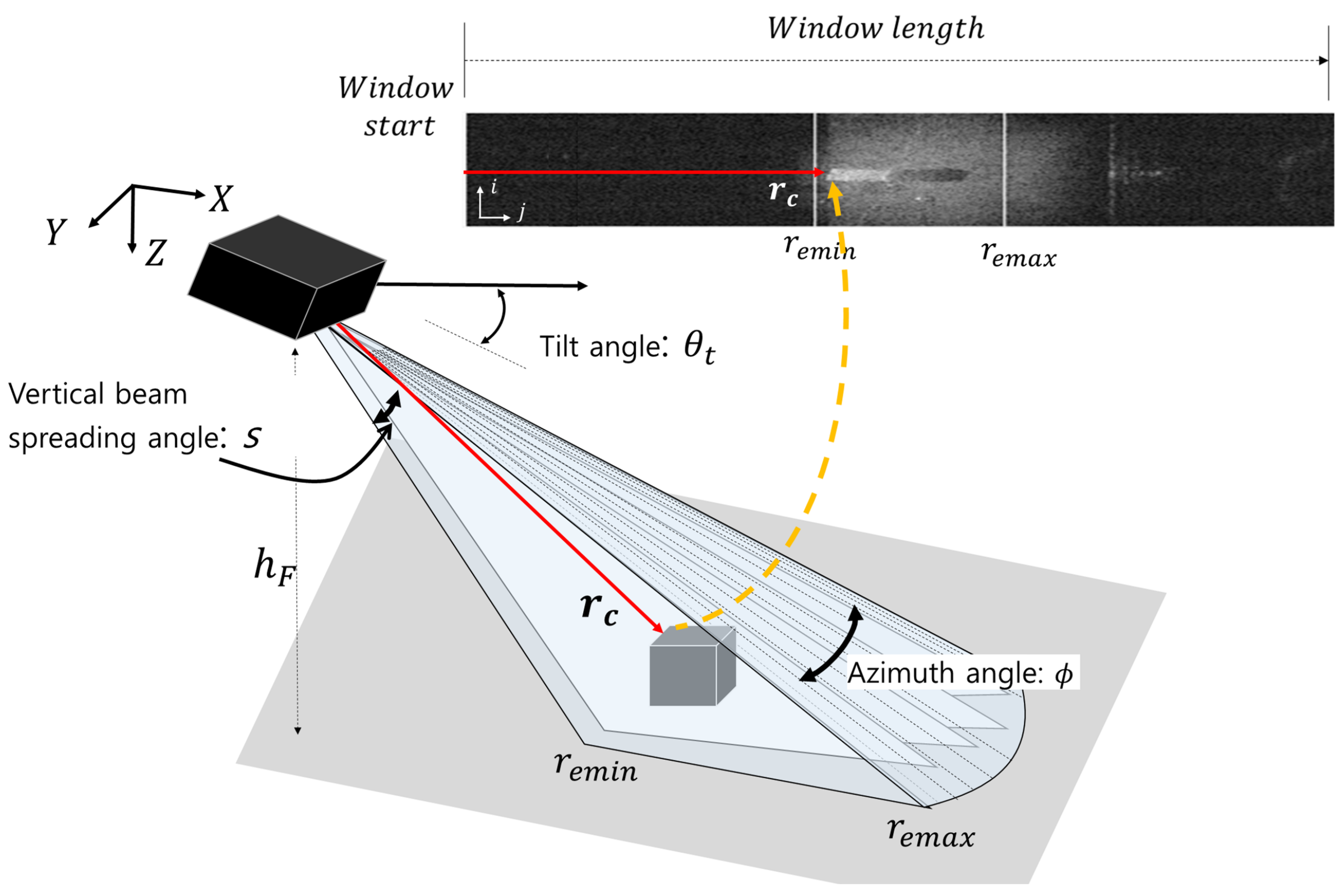
2.1. Characteristics of Sonar Imaging
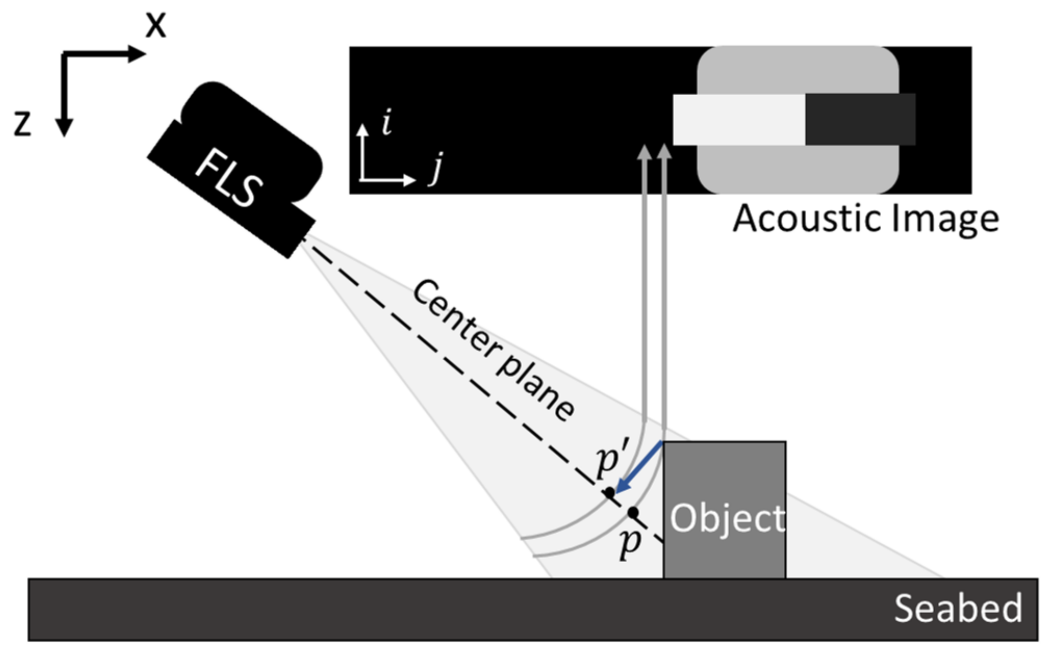
2.2. Limitation in the Single-Sonar Method
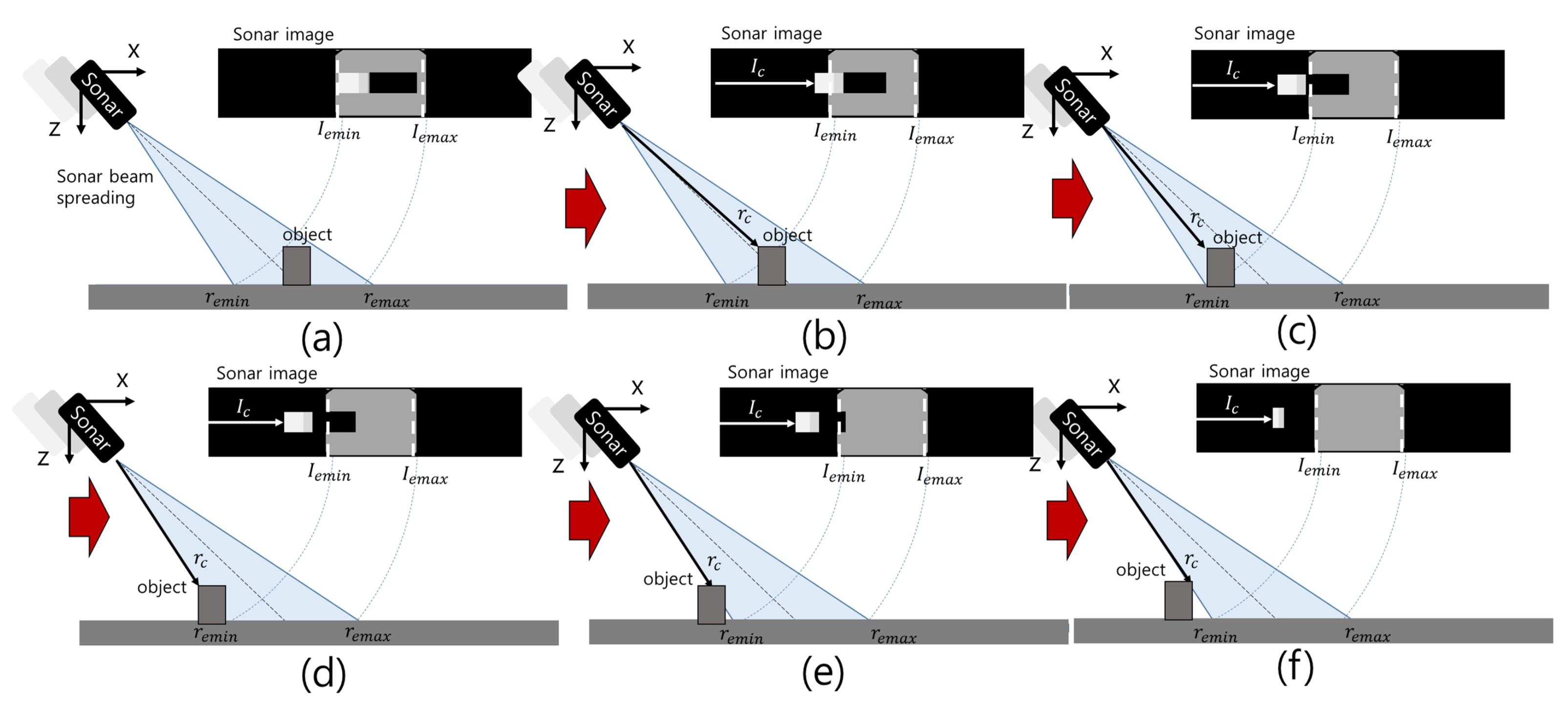
2.3. Proposed Method
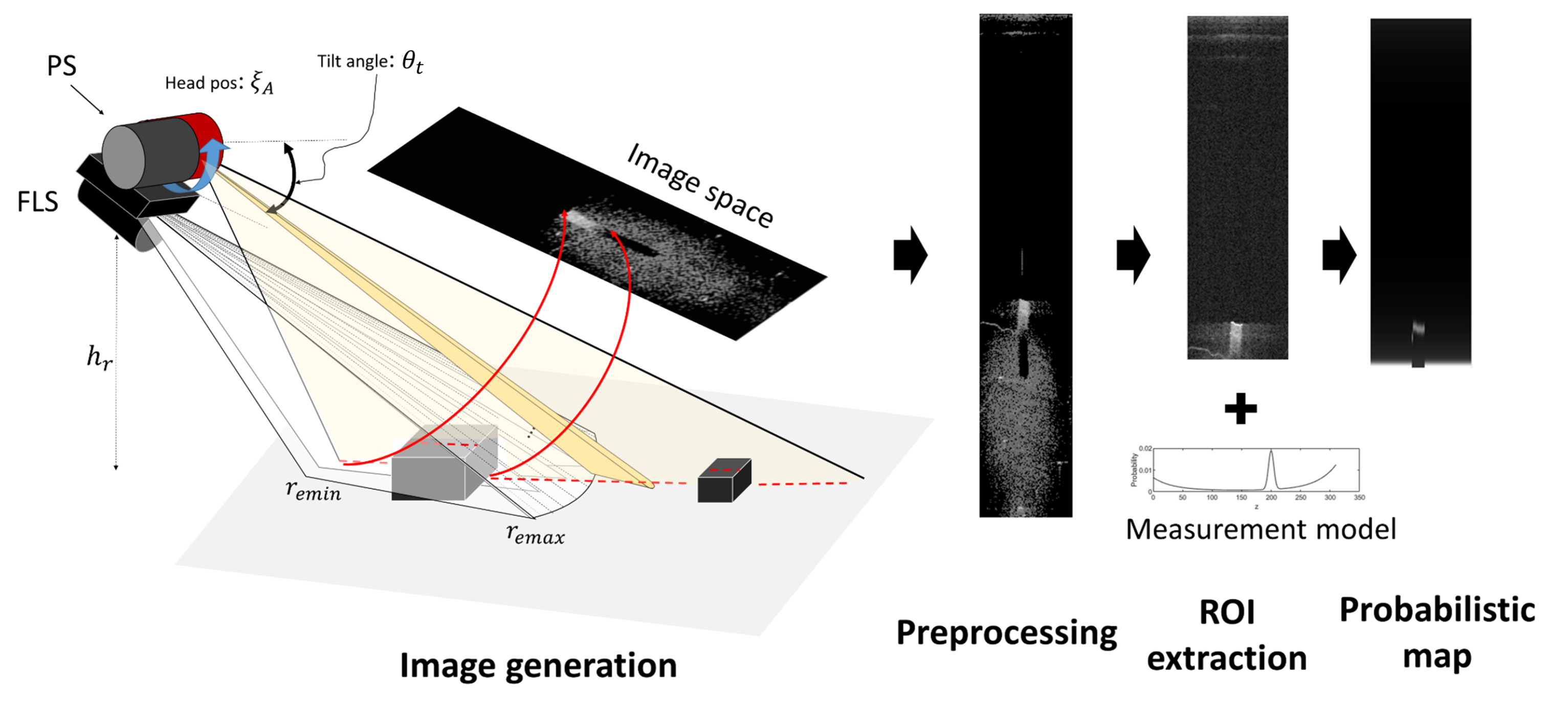
2.4. Region of Interest
2.5. Sonar Measurement Model
2.6. Likelihood Field Generation
3. Validation
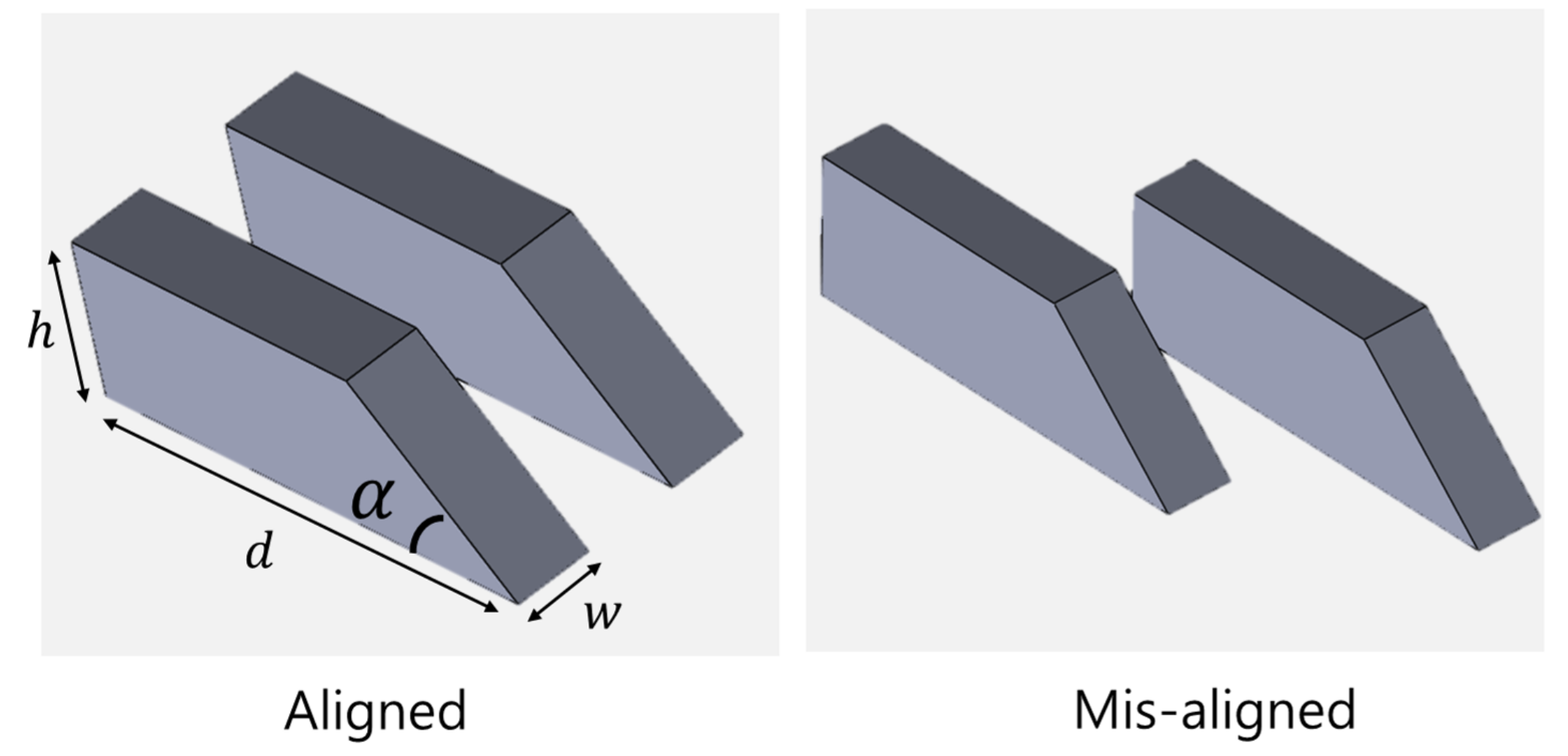
3.1. Simulation
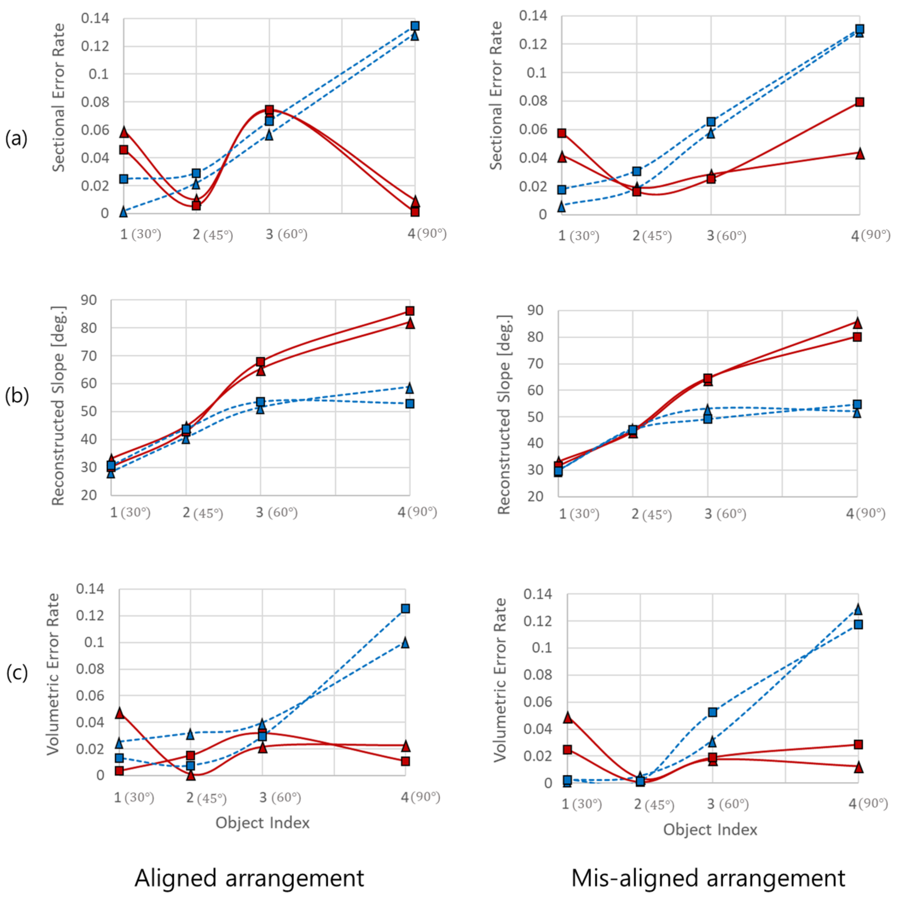
3.2. Simulation Results
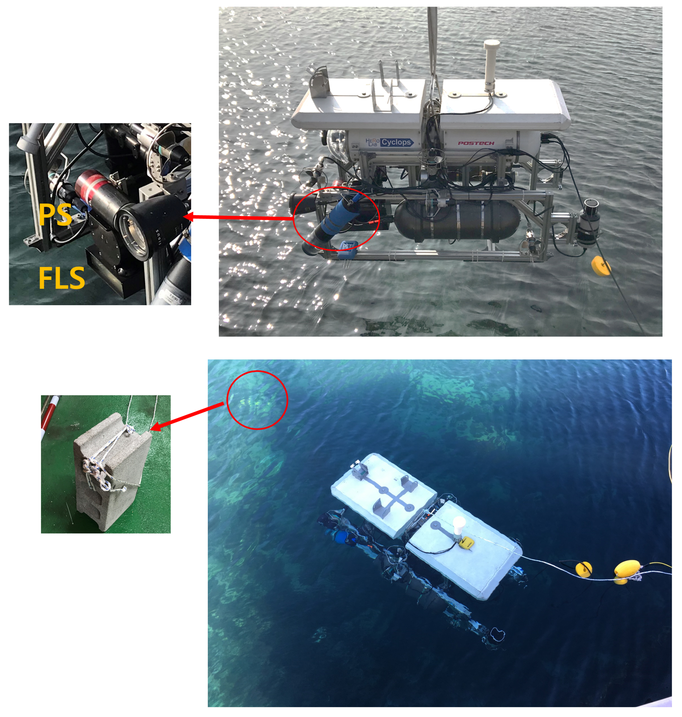
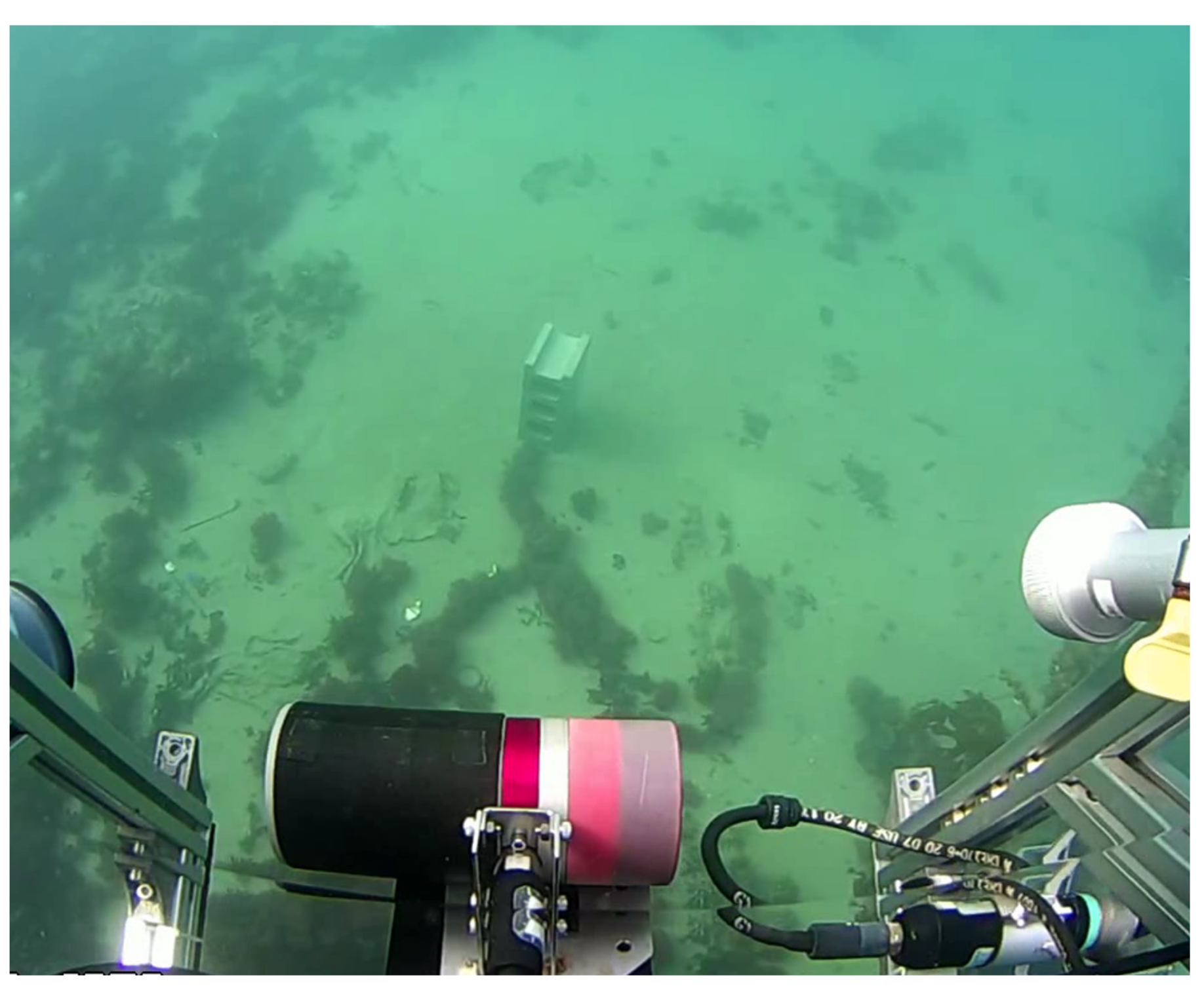
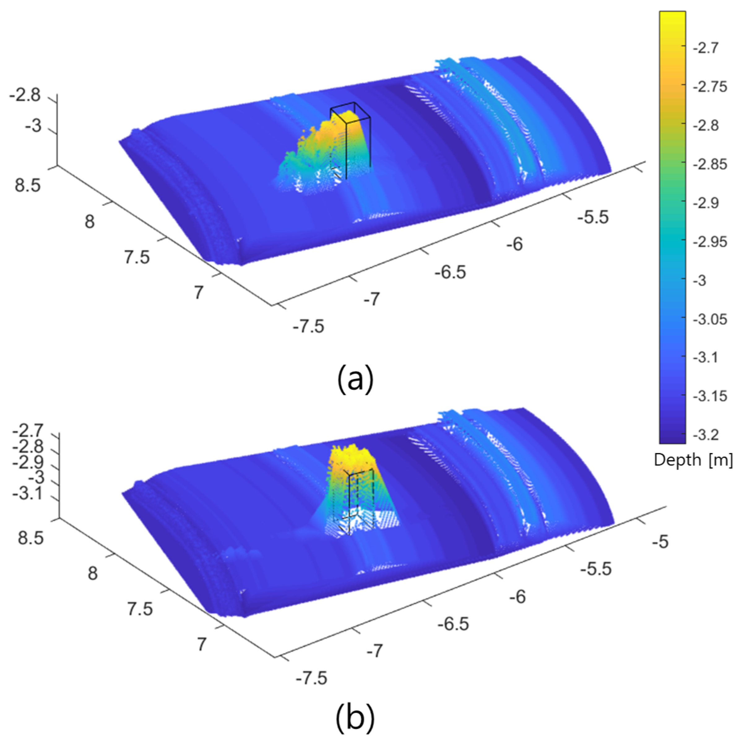
3.3. Experiment
4. Conclusions
Author Contributions
Funding
Institutional Review Board Statement
Informed Consent Statement
Data Availability Statement
Conflicts of Interest
References
- Belcher, E.; Hanot, W.; Burch, J. Dual-frequency identification sonar (DIDSON). In Proceedings of the Proceedings of the 2002 Interntional Symposium on Underwater Technology, (Cat. No. 02EX556). Tokyo, Japan, 19 April 2002; pp. 187–192. [Google Scholar]
- Wang, X.; Wang, L.; Li, G.; Xie, X. A Robust and Fast Method for Sidescan Sonar Image Segmentation Based on Region Growing. Sensors 2021, 21, 6960. [Google Scholar] [CrossRef] [PubMed]
- Coiras, E.; Groen, J. 3D Target Shape from SAS Images Based on a Deformable Mesh; NURC: Kigali, Rwanda, 2009; NURC-PR-2009-001. [Google Scholar]
- Moszyński, M.; Bikonis, K.; Lubniewski, Z. Reconstruction of 3D shape from sidescan sonar images using shape from shading technique. Hydroacoustics 2013, 16, 181–188. [Google Scholar]
- Huang, T.A.; Kaess, M. Towards acoustic structure from motion for imaging sonar. In Proceedings of the 2015 IEEE/RSJ International Conference on Intelligent Robots and Systems (IROS), Hamburg, Germany, 28 September–2 October 2015; pp. 758–765. [Google Scholar]
- Huang, T.A.; Kaess, M. Incremental data association for acoustic structure from motion. In Proceedings of the 2016 IEEE/RSJ International Conference on Intelligent Robots and Systems (IROS), Daejeon, Korea, 9–14 October 2016; pp. 1334–1341. [Google Scholar]
- Storlazzi, C.D.; Dartnell, P.; Hatcher, G.A.; Gibbs, A.E. End of the chain? Rugosity and fine-scale bathymetry from existing underwater digital imagery using structure-from-motion (SfM) technology. Coral Reefs 2016, 35, 889–894. [Google Scholar] [CrossRef]
- Aykin, M.D.; Negahdaripour, S. Three-dimensional target reconstruction from multiple 2-d forward-scan sonar views by space carving. IEEE J. Ocean. Eng. 2016, 42, 574–589. [Google Scholar] [CrossRef]
- Negahdaripour, S. Application of forward-scan sonar stereo for 3-D scene reconstruction. IEEE J. Ocean. Eng. 2018, 45, 547–562. [Google Scholar] [CrossRef]
- Guerneve, T.; Subr, K.; Petillot, Y. Three-dimensional reconstruction of underwater objects using wide-aperture imaging SONAR. J. Field Robot. 2018, 35, 890–905. [Google Scholar] [CrossRef]
- Cho, H.; Kim, B.; Yu, S.C. AUV-based underwater 3-D point cloud generation using acoustic lens-based multibeam sonar. IEEE J. Ocean. Eng. 2017, 43, 856–872. [Google Scholar] [CrossRef]
- Joe, H.; Cho, H.; Sung, M.; Kim, J.; Yu, S.c. Sensor fusion of two sonar devices for underwater 3D mapping with an AUV. Auton. Robot. 2021, 45, 543–560. [Google Scholar] [CrossRef]
- Joe, H.; Kim, J.; Yu, S.C. 3D reconstruction using two sonar devices in a Monte-Carlo approach for AUV application. Int. J. Control Autom. Syst. 2020, 18, 587–596. [Google Scholar] [CrossRef]
- Sung, M.; Kim, J.; Cho, H.; Lee, M.; Yu, S.C. Underwater-Sonar-Image-Based 3D Point Cloud Reconstruction for High Data Utilization and Object Classification Using a Neural Network. Electronics 2020, 9, 1763. [Google Scholar] [CrossRef]
- Walter, M.R. Sparse Bayesian Information Filters for Localization and Mapping. Ph.D. Thesis, Massachusetts Institute of Technology, Cambridge, MA, USA, 2008. [Google Scholar]
- Hurtós Vilarnau, N. Forward-Looking Sonar Mosaicing for Underwater Environments. Ph.D. Thesis, Universitat de Girona, Girona, Spain, 2014. [Google Scholar]
- Gu, J.H.; Joe, H.G.; Yu, S.C. Development of image sonar simulator for underwater object recognition. In Proceedings of the 2013 OCEANS-San Diego, San Diego, CA, USA, 23–27 September 2013; pp. 1–6. [Google Scholar]
- Kim, J.; Sung, M.; Yu, S.C. Development of simulator for autonomous underwater vehicles utilizing underwater acoustic and optical sensing emulators. In Proceedings of the 2018 18th International Conference on Control, Automation and Systems (ICCAS), PyeongChang, Korea, 17–20 October 2018; pp. 416–419. [Google Scholar]
- Pyo, J.; Cho, H.; Joe, H.; Ura, T.; Yu, S.C. Development of hovering type AUV “Cyclops” and its performance evaluation using image mosaicing. Ocean. Eng. 2015, 109, 517–530. [Google Scholar] [CrossRef] [Green Version]
- Rigby, P.; Pizarro, O.; Williams, S.B. Towards geo-referenced AUV navigation through fusion of USBL and DVL measurements. In Proceedings of the OCEANS 2006, Boston, MA, USA, 18–21 September 2006; pp. 1–6. [Google Scholar]
- Joe, H.; Kim, M.; Yu, S.C. Second-order sliding-mode controller for autonomous underwater vehicle in the presence of unknown disturbances. Nonlinear Dyn. 2014, 78, 183–196. [Google Scholar] [CrossRef]


| Object | Front Slope [Degrees] | Dimensions (W × H × D) [m] |
|---|---|---|
| 1 | 90 | 0.5 × 1 × 1.6 |
| 2 | 80 | 0.5 × 1 × 1.6 |
| 3 | 60 | 0.5 × 1 × 1.6 |
| 4 | 45 | 0.5 × 1 × 2 |
| 5 | 30 | 0.5 × 1 × 3 |
| 6 | 20 | 0.5 × 1 × 3 |
| Object Index | Front Slope | Size (W × H × D, [m]) | Sectional Area [m] | Volume [m] |
|---|---|---|---|---|
| 1 | 30 | 0.5 × 1 × 3 | 2.13 | 1.07 |
| 2 | 45 | 0.5 × 1 × 3 | 2.5 | 1.25 |
| 3 | 60 | 0.5 × 1 × 3 | 2.71 | 1.36 |
| 4 | 90 | 0.5 × 1 × 3 | 3 | 1.5 |
Publisher’s Note: MDPI stays neutral with regard to jurisdictional claims in published maps and institutional affiliations. |
© 2022 by the authors. Licensee MDPI, Basel, Switzerland. This article is an open access article distributed under the terms and conditions of the Creative Commons Attribution (CC BY) license (https://creativecommons.org/licenses/by/4.0/).
Share and Cite
Joe, H.; Kim, J.; Yu, S.-C. Probabilistic 3D Reconstruction Using Two Sonar Devices. Sensors 2022, 22, 2094. https://doi.org/10.3390/s22062094
Joe H, Kim J, Yu S-C. Probabilistic 3D Reconstruction Using Two Sonar Devices. Sensors. 2022; 22(6):2094. https://doi.org/10.3390/s22062094
Chicago/Turabian StyleJoe, Hangil, Jason Kim, and Son-Cheol Yu. 2022. "Probabilistic 3D Reconstruction Using Two Sonar Devices" Sensors 22, no. 6: 2094. https://doi.org/10.3390/s22062094