
Modified U-NET Architecture for Segmentation of Skin Lesion

 ,
,  and
and
Abstract
:1. Introduction
- A modified U-Net architecture has been proposed for the segmentation of lesions from skin disease using dermoscopy images.
- The data augmentation technique has been performed to increase the randomness of images for better stability.
- The proposed model is validated with different optimizers, batch sizes, and epochs for better accuracy.
- The proposed model has been analyzed with various performance parameters such as Jaccard Index, Dice Coefficient, Precision, Recall, Accuracy and Loss.
2. Materials and Methods
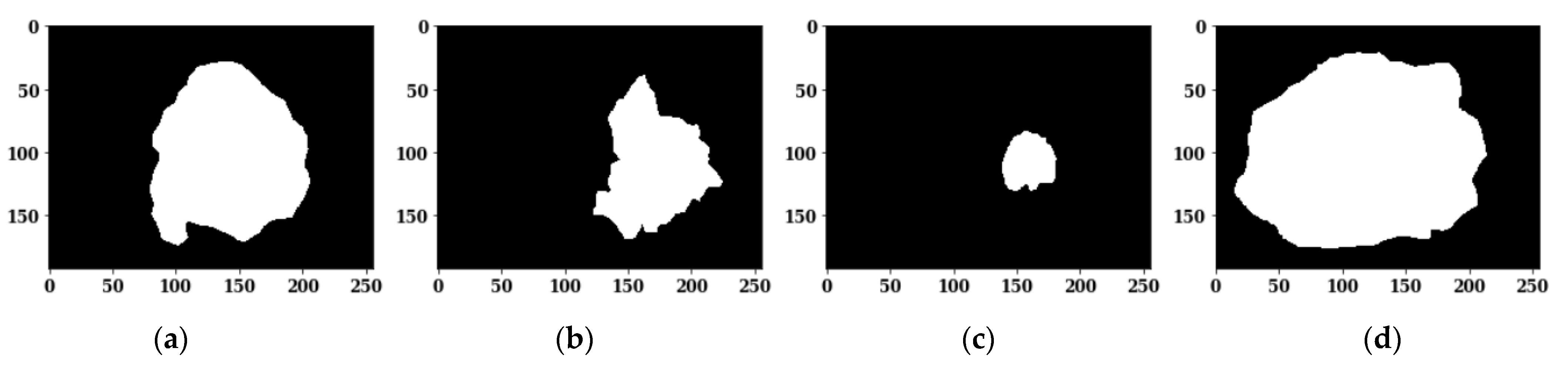
2.1. Dataset
2.2. Data Augmentation
2.3. Modified U-Net Architecture
3. Results and Discussion
3.1. Result Analysis Based on Different Optimizers
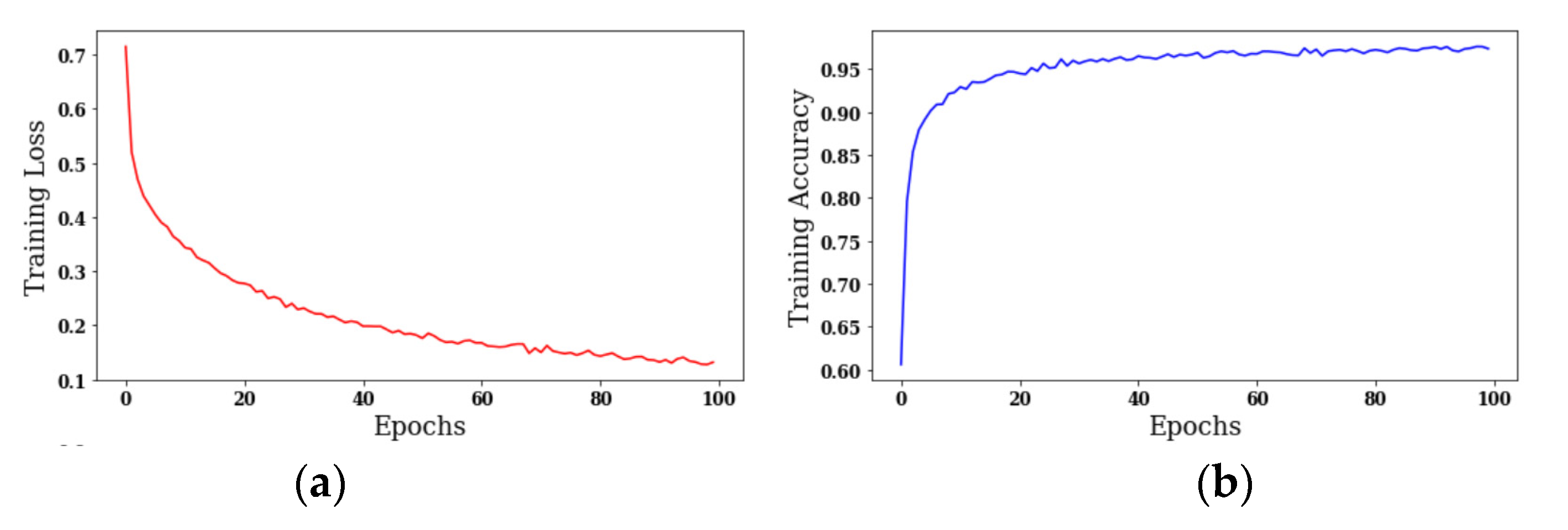
3.1.1. Analysis of Training Loss and Accuracy
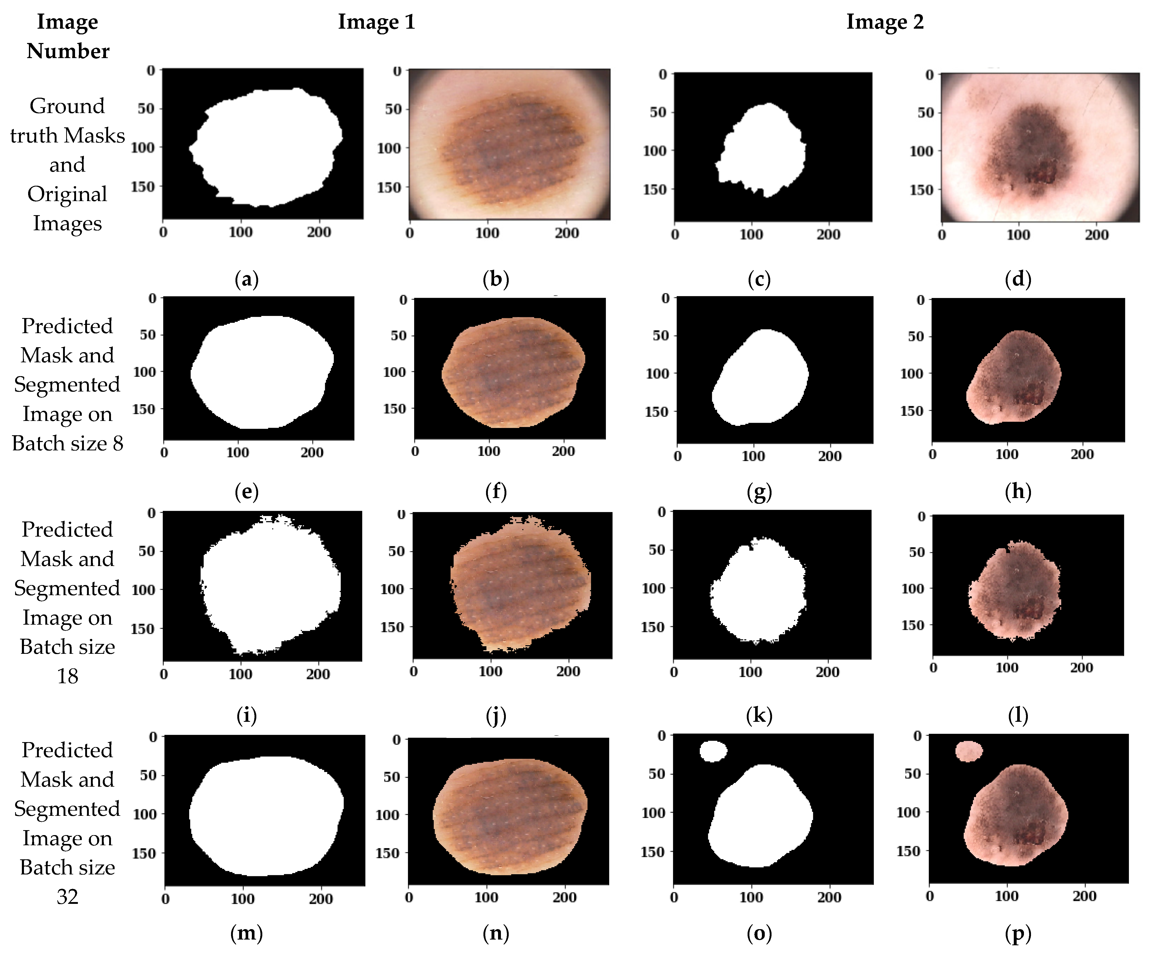
3.1.2. Visual Analysis of Segmented Images
3.1.3. Analysis of Confusion Matrix Parameters
3.2. Result Analysis Based on Different Optimizers
3.2.1. Analysis of Training Loss and Accuracy
3.2.2. Analysis of Training Loss and Accuracy
3.2.3. Analysis of Confusion Matrix Parameters
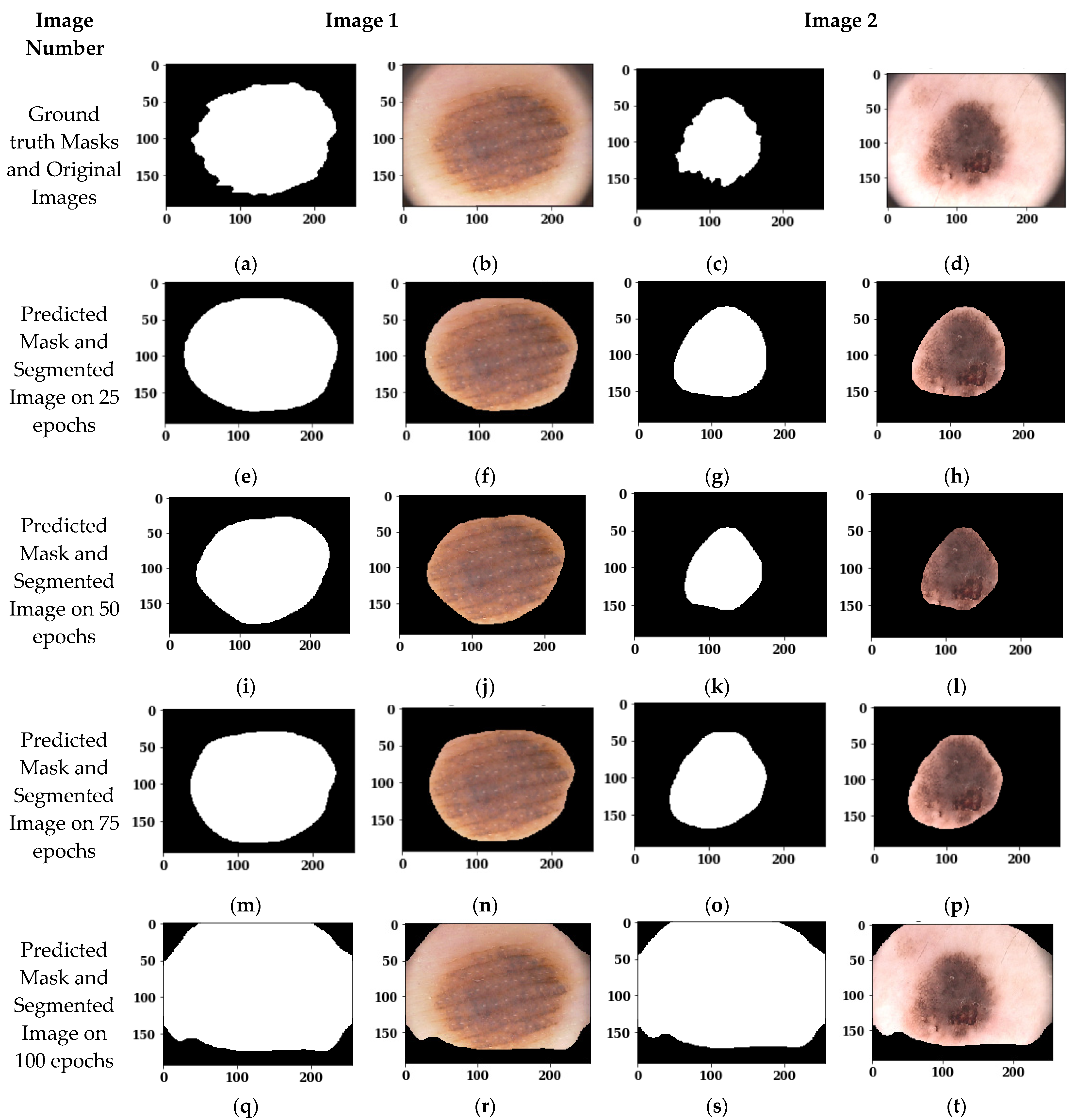
3.3. Result Analysis Based on Different Epochs with the Adam Optimizer and Batch Size 8
3.3.1. Analysis of Confusion Matrix Parameters
3.3.2. Visual Analysis of Segmented Images
3.3.3. Analysis of Confusion Matrix Parameters
3.4. Comparison with State-of-the-Art Techniques
4. Conclusions and Future Scope
Author Contributions
Funding
Institutional Review Board Statement
Informed Consent Statement
Data Availability Statement
Conflicts of Interest
References
- Anand, V.; Gupta, S.; Koundal, D. Skin Disease Diagnosis: Challenges and Opportunities. In Advances in Intelligent Systems and Computing, Proceedings of the Second Doctoral Symposium on Computational Intelligence, Lucknow, India, 5 March 2022; Springer: Singapore, 2022; Volume 1374, p. 1374. [Google Scholar]
- Shinde, P.P.; Seema, S. A Review of Machine Learning and Deep Learning Applications. In Proceedings of the 2018 Fourth International Conference on Computing Communication Control and Automation (ICCUBEA), Pune, India, 16–18 August 2018; pp. 1–6. [Google Scholar]
- Goyal, A. Around 19 Crore Indians Likely to Suffer from Skin Diseases by 2015-Notes Frost & Sullivan. 2014. Available online: https://www.freepressjournal.in/business-wire-india-section/around-19-crore-indians-likely-to-suffer-from-skin-diseases-by-2015-notes-frost-sullivan (accessed on 28 November 2021).
- Liu, L.; Tsui, Y.Y.; Mandal, M. Skin lesion segmentation using deep learning with auxiliary task. J. Imaging 2021, 7, 67. [Google Scholar] [CrossRef]
- Liu, L.; Mou, L.; Zhu, X.X.; Mandal, M. Automatic skin lesion classification based on mid-level feature learning. Comput. Med. Imaging Graph. 2020, 84, 101765. [Google Scholar] [CrossRef]
- Li, Y.; Shen, L. Skin lesion analysis towards melanoma detection using deep learning network. Sensors 2018, 18, 556. [Google Scholar] [CrossRef] [Green Version]
- Singh, V.K.; Abdel-Nasser, M.; Rashwan, H.A.; Akram, F.; Pandey, N.; Lalande, A.; Presles, B.; Romani, S.; Puig, D. FCA-Net: Adversarial learning for skin lesion segmentation based on multi-scale features and factorized channel attention. IEEE Access 2019, 7, 130552–130565. [Google Scholar] [CrossRef]
- Yang, X.; Zeng, Z.; Yeo, S.Y.; Tan, C.; Tey, H.L.; Su, Y. A novel multi-task deep learning model for skin lesion segmentation and Classification. arXiv 2017, arXiv:1703.01025. [Google Scholar]
- Xie, Y.; Zhang, J.; Xia, Y.; Shen, C. A mutual bootstrapping model for automated skin lesion segmentation and classification. IEEE Trans. Med. Imaging 2020, 39, 2482–2493. [Google Scholar] [CrossRef] [Green Version]
- Yuan, Y.; Chao, M.; Lo, Y.-C. Automatic skin lesion segmentation using deep fully convolution networks with Jaccard distance. IEEE Trans. Med. Imaging 2017, 36, 1876–1886. [Google Scholar] [CrossRef]
- Yuan, Y. Automatic skin lesion segmentation with fully convolutional-deconvolutional networks. arXiv 2017, arXiv:1703.05165. [Google Scholar]
- Schaefer, G.; Rajab, M.I.; Celebi, M.E.; Iyatomi, H. Colour and contrast enhancement for improved skin lesion segmentation. Comput. Med. Imaging Graph. 2011, 35, 99–104. [Google Scholar] [CrossRef]
- Bi, L.; Kim, J.; Ahn, E.; Kumar, A.; Fulham, M.; Feng, D. Dermoscopic image segmentation via multi-stage fully convolutional networks. IEEE Trans. Biomed. Eng. 2017, 64, 2065–2074. [Google Scholar] [CrossRef] [Green Version]
- Liu, X.; Song, L.; Liu, S.; Zhang, Y. A review of deep-learning-based medical image segmentation methods. Sustainability 2021, 13, 1224. [Google Scholar] [CrossRef]
- Shankar, K.; Zhang, Y.; Liu, Y.; Wu, L.; Chen, C.H. Hyperparameter tuning deep learning for diabetic retinopathy fundus image classification. IEEE Access 2020, 8, 118164–118173. [Google Scholar] [CrossRef]
- Pustokhina, I.V.; Pustokhin, D.A.; Gupta, D.; Khanna, A.; Shankar, K.; Nguyen, G.N. An effective training scheme for deep neural network in edge computing enabled Internet of Medical Things (IoMT) systems. IEEE Access 2020, 8, 107112–107123. [Google Scholar] [CrossRef]
- Raj, R.J.S.; Shobana, S.J.; Pustokhina, I.V.; Pustokhin, D.A.; Gupta, D.; Shankar, K. Optimal feature selection-based medical image classification using deep learning model in internet of medical things. IEEE Access 2020, 8, 58006–58017. [Google Scholar] [CrossRef]
- Anand, V.; Koundal, D. Computer-assisted diagnosis of thyroid cancer using medical images: A survey. In Proceedings of ICRIC 2019; Springer: Cham, Switzerland, 2019; pp. 543–559. [Google Scholar]
- Garnavi, R.; Aldeen, M.; Celebi, M.E.; Varigos, G.; Finch, S. Border detection in dermoscopy images using hybrid thresholding on optimized color channels. Comput. Med. Imaging Graph. 2011, 35, 105–115. [Google Scholar] [CrossRef]
- Ganster, H.; Pinz, P.; Rohrer, R.; Wildling, E.; Binder, M.; Kittler, H. Automated melanoma recognition. IEEE Trans. Med. Imaging 2001, 20, 233–239. [Google Scholar] [CrossRef]
- Erkol, B.; Moss, R.H.; Stanley, R.J.; Stoecker, W.V.; Hva-tum, E. Automatic lesion boundary detection in dermoscopy images using gradient vector flow snakes. Skin Res. Technol. 2005, 11, 17–26. [Google Scholar] [CrossRef] [Green Version]
- She, Z.; Liu, Y.; Damatoa, A. Combination of features from skin pattern and ABCD analysis for lesion classification. Ski. Res. Technol. 2007, 13, 25–33. [Google Scholar] [CrossRef] [Green Version]
- Celebi, M.E.; Wen QU, A.N.; Iyatomi Shimizu Zhou, H.; Schaefer, G. A state-of-the-art survey on lesion border detection in dermoscopy images. Dermoscopy Image Anal. 2015, 10, 97–129. [Google Scholar]
- Koohbanani, N.A.; Jahanifar, M.; Tajeddin, N.Z.; Gooya, A.; Rajpoot, N. Leveraging transfer learning for segmenting lesions and their attributes in dermoscopy images. arXiv 2018, arXiv:1809.10243. [Google Scholar]
- Masni, A.; Mohammed, A.; Kim, D.H.; Kim, T.S. Multiple skin lesions diagnostics via integrated deep convolutional networks for segmentation and classification. Comput. Methods Programs Biomed. 2020, 190, 105351. [Google Scholar] [CrossRef]
- Dorj, U.O.; Lee, K.K.; Choi, J.Y.; Lee, M. The skin cancer classification using deep convolutional neural network. Multimed. Tools Appl. 2018, 77, 9909–9924. [Google Scholar] [CrossRef]
- Mishra, S.; Tripathy, H.K.; Mallick, P.K.; Bhoi, A.K.; Barsocchi, P. EAGA-MLP—An enhanced and adaptive hybrid classification model for diabetes diagnosis. Sensors 2020, 20, 4036. [Google Scholar] [CrossRef]
- Roy, S.; Poonia, R.C.; Nayak, S.R.; Kumar, R.; Alzahrani, K.J.; Alnfiai, M.M.; Al-Wesabi, F.N. Evaluating the Usability of mHealth Applications on Type-2 Diabetes Mellitus using various MCDM Models. Healthcare 2022, 10, 4. [Google Scholar]
- Srinivasu, P.N.; Bhoi, A.K.; Nayak, S.R.; Bhutta, M.R.; Woźniak, M. Block-chain Technology for Secured Healthcare Data Communication among the Non-Terminal nodes in IoT architecture in 5G Network. Electronics 2021, 10, 1437. [Google Scholar] [CrossRef]
- Satapathy, S.K.; Bhoi, A.K.; Loganathan, D.; Khandelwal, B.; Barsocchi, P. Machine learning with ensemble stacking model for automated sleep staging using dual-channel EEG signal. Biomed. Signal Process. Control. 2021, 69, 102898. [Google Scholar] [CrossRef]
- Pramanik, M.; Pradhan, R.; Nandy, P.; Bhoi, A.K.; Barsocchi, P. Machine Learning Methods with Decision Forests for Parkinson’s Detection. Appl. Sci. 2021, 11, 581. [Google Scholar] [CrossRef]
- Saxena, U.; Moulik, S.; Nayak, S.R.; Hanne, T.; Sinha Roy, D. Ensemble-Based Machine Learning for Predicting Sudden Human Fall Using Health Data. Math. Probl. Eng. 2021, 2021, 8608630. [Google Scholar] [CrossRef]
- Garg, M.; Gupta, S.; Nayak, S.R.; Nayak, J.; Pelusi, D. Modified Pixel Level Snake using Bottom Hat Transformation for Evolution of Retinal Vasculature Map. Math. Biosci. Eng. 2021, 18, 5737–5757. [Google Scholar] [CrossRef]
- Li, H.; He, X.; Zhou, F.; Yu, Z.; Ni, D.; Chen, S.; Wang, T.; Lei, B. Dense deconvolutional network for skin lesion segmentation. IEEE J. Biomed. Health Inform. 2018, 23, 527–537. [Google Scholar] [CrossRef]
- Kathiresan, S.; Sait, A.R.W.; Gupta, D.; Lakshmanaprabu, S.K.; Khanna, A.; Pandey, H.M. Automated detection and classification of fundus diabetic retinopathy images using synergic deep learning model. Pattern. Recogn. Lett. 2020, 133, 210–216. [Google Scholar]
- Yu, Z.; Jiang, X.; Zhou, F.; Qin, J.; Ni, D.; Chen, S.; Lei, B.; Wang, T. Melanoma recognition in dermoscopy images via aggregated deep convolutional features. IEEE Trans. Biomed. Eng. 2018, 66, 1006–1016. [Google Scholar] [CrossRef]
- Khan, A.H.; Iskandar, D.A.; Al-Asad, J.F.; El-Nakla SAMIRAnd Alhuwaidi, S.A. Statistical Feature Learning through Enhanced Delaunay Clustering and Ensemble Classifiers for Skin Lesion Segmentation and Classification. J. Theor. Appl. Inf. Technol. 2021, 99. [Google Scholar]
- Long, J.; Shelhamer, E.; Darrell, T. Fully convolutional networks for semantic segmentation. In Proceedings of the IEEE Conference on Computer Vision and Pattern Recognition 2015, Boston, MA, USA, 7–12 June 2015; pp. 3431–3440. [Google Scholar]
- Chen, L.C.; Papandreou, G.; Kokkinos, I.; Murphy, K.; Yuille, A.L. Semantic image segmentation with deep convolutional nets and fully connected crfs. arXiv 2014, arXiv:1412.7062. [Google Scholar]
- Noh, H.; Hong, S.; Han, B. Learning deconvolution network for semantic segmentation. In Proceedings of the IEEE International Conference on Computer Vision, Santiago, Chile, 7–13 December 2015; pp. 1520–1528. [Google Scholar]
- Wang, Z.; Zou, N.; Shen, D.; Ji, S. Non-local u-nets for biomedical image segmentation. Proc. AAAI Conf. Artif. Intell. 2020, 34, 6315–6322. [Google Scholar] [CrossRef]
- Ibtehaz, N.; Rahman, M.S. MultiResUNet: Rethinking the U-Net architecture for multimodal biomedical image segmentation. Neural Netw. 2020, 121, 74–87. [Google Scholar] [CrossRef]
- Christ, P.F.; Elshaer, M.E.A.; Ettlinger, F.; Tatavarty, S.; Bickel, M.; Bilic, P.; Rempfler, M.; Armbruster, M.; Hofmann, F.; D’Anastasi, M.; et al. Automatic liver and lesion segmentation in CT using cascaded fully convolutional neural networks and 3D conditional random fields. In Proceedings of the International Conference on Medical Image Computing and Computer-Assisted Intervention, Athens, Greece, 17–21 October 2016; Springer: Cham, Switzerland, 2016; pp. 415–423. [Google Scholar]
- Lin, G.; Milan, A.; Shen, C.; Reid, I. Refinenet: Multi-path refinement networks for high-resolution semantic segmentation. In Proceedings of the IEEE Conference on Computer Vision and Pattern Recognition, Honolulu, HI, USA, 21–26 July 2017; pp. 1925–1934. [Google Scholar]
- Novikov, A.A.; Lenis, D.; Major, D.; Hladůvka, J.; Wimmer, M.; Bühler, K. Fully convolutional architectures for multiclass segmentation in chest radiographs. IEEE Trans. Med. Imaging 2018, 37, 1865–1876. [Google Scholar] [CrossRef] [Green Version]
- Mendonca, T.; Celebi, M.; Marques, J. Ph2: A Public Database for the Analysis of Dermoscopic Images. Dermoscopy Image Analysis. 2015. Available online: https://www.taylorfrancis.com/chapters/mono/10.1201/b19107-17/ph2-public-database-analysis-dermoscopic-images-emre-celebi-teresa-mendonca-jorge-marques (accessed on 28 November 2021).
- Shorten, C.C.; Khoshgoftaar, M.T. A Survey on Image Data Augmentation for Deep Learning. J. Big Data 2019, 6, 60. [Google Scholar] [CrossRef]
- Ronneberger, O.; Fischer, P.; Brox, T. U-net: Convolutional networks for biomedical image segmentation. In International Conference on Medical image computing and computer-assisted intervention. arXiv 2015, arXiv:1505.04597. [Google Scholar]


| S. No. | Layers | Input Image Size | Filter Size | No. of Filter | Activation Function | Output Image Size | Parameters |
|---|---|---|---|---|---|---|---|
| 1 | Input Image | 192 × 256 × 3 | - | - | - | - | - |
| 2 | Conv_1 | 192 × 256 × 3 | 3 × 3 | 64 | ReLU | 192 × 256 × 64 | 1792 |
| 3 | Batch Normalization | 192 × 256 × 64 | - | - | - | - | 256 |
| 4 | Conv 2 | 192 × 256 × 3 | 3 × 3 | 64 | ReLU | 192 × 256 × 64 | 36,928 |
| 5 | Batch Normalization | 192 × 256 × 64 | - | - | - | - | 256 |
| 6 | MaxPooling | 192 × 256 × 64 | 3 × 3 | - | - | 96 × 128 × 64 | 0 |
| 7 | Conv_3 | 96 × 128 × 128 | 3 × 3 | 128 | ReLU | 96 × 128 × 128 | 73,856 |
| 8 | Batch Normalization | 96 × 128 × 128 | - | - | - | - | 512 |
| 9 | Conv 4 | 96 × 128 × 128 | 3 × 3 | 128 | ReLU | 96 × 128 × 128 | 147,584 |
| 10 | Batch Normalization | 96 × 128 × 128 | - | - | - | - | 512 |
| 11 | MaxPooling | 96 × 128 × 128 | 3 × 3 | - | - | 48 × 64 × 128 | 0 |
| 12 | Conv 5 | 48 × 64 × 256 | 3 × 3 | 256 | ReLU | 48 × 64 × 256 | 295,168 |
| 13 | Batch Normalization | 48 × 64 × 256 | - | - | - | - | 1024 |
| 14 | Conv 6 | 48 × 64 × 256 | 3 × 3 | 256 | ReLU | 96 × 128 × 128 | 590,080 |
| 15 | Batch Normalization | 48 × 64 × 256 | - | - | - | - | 1024 |
| 16 | MaxPooling | 48 × 64 × 256 | 3 × 3 | - | - | 48 × 64 × 128 | |
| 17 | Conv 7 | 48 × 64 × 256 | 3 × 3 | 256 | ReLU | 96 × 128 × 128 | 590,080 |
| 18 | Batch Normalization | 48 × 64 × 256 | - | - | - | - | 1024 |
| 19 | MaxPooling | 48 × 64 × 256 | 3 × 3 | - | - | 24 × 32 × 256 | 0 |
| 20 | Conv 8 | 24 × 32 × 512 | 3 × 3 | 512 | ReLU | 24 × 32 × 512 | 1,180,160 |
| 21 | Batch Normalization | 24 × 32 × 512 | - | - | - | - | 2048 |
| 22 | Conv 9 | 24 × 32 × 512 | 3 × 3 | 512 | ReLU | 24 × 32 × 512 | 2,359,808 |
| 23 | Batch Normalization | 24 × 32 × 512 | - | - | - | - | 2048 |
| 24 | Conv 10 | 24 × 32 × 512 | 3 × 3 | 512 | ReLU | 24 × 32 × 512 | 2,359,808 |
| 25 | Batch Normalization | 24 × 32 × 512 | - | - | - | - | 2048 |
| 26 | MaxPooling | 24 × 32 × 512 | 3 × 3 | - | - | 12 × 16 × 512 | 0 |
| 27 | Conv 11 | 12 × 16 × 512 | 3 × 3 | 512 | ReLU | 12 × 16 × 512 | 2,359,808 |
| 28 | Batch Normalization | 12 × 16 × 512 | - | - | - | - | 2048 |
| 29 | Conv 12 | 12 × 16 × 512 | 3 × 3 | 512 | ReLU | 12 × 16 × 512 | 2,359,808 |
| 30 | Batch Normalization | 12 × 16 × 512 | - | - | - | - | 2048 |
| 31 | Conv 13 | 12 × 16 × 512 | 3 × 3 | 512 | ReLU | 12 × 16 × 512 | 2,359,808 |
| 32 | Batch Normalization | 12 × 16 × 512 | - | - | - | - | 2048 |
| 33 | MaxPooling | 12 × 16 × 512 | 3 × 3 | - | - | 6 × 8 × 512 | 0 |
| 34 | Upsampling | 12 × 16 × 1024 | - | - | - | 12 × 16 × 1024 | 0 |
| 35 | De-Conv 1 | 12 × 16 × 512 | 3 × 3 | 512 | ReLU | 12 × 16 × 512 | 4,719,104 |
| 36 | Batch Normalization | 12 × 16 × 512 | - | - | - | - | 2048 |
| 37 | De-Conv 2 | 12 × 16 × 512 | 3 × 3 | 512 | ReLU | 12 × 16 × 512 | 2,359,808 |
| 38 | Batch Normalization | 12 × 16 × 512 | - | - | - | - | 2048 |
| 39 | De-Conv 3 | 12 × 16 × 512 | 3 × 3 | 512 | ReLU | 12 × 16 × 512 | 2,359,808 |
| 40 | Batch Normalization | 12 × 16 × 512 | - | - | - | - | 2048 |
| 41 | Upsampling | 24 × 32 × 512 | - | - | - | 24 × 32 × 512 | 0 |
| 42 | De-Conv 4 | 24 × 32 × 512 | 3 × 3 | 512 | ReLU | 24 × 32 × 512 | 2,359,808 |
| 43 | Batch Normalization | 24 × 32 × 512 | - | - | - | - | 2048 |
| 44 | De-Conv 5 | 24 × 32 × 512 | 3 × 3 | 512 | ReLU | 24 × 32 × 512 | 2,359,808 |
| 45 | Batch Normalization | 24 × 32 × 512 | - | - | - | - | 2048 |
| 46 | De-Conv 6 | 24 × 32 × 256 | 3 × 3 | 512 | ReLU | 24 × 32 × 512 | 1,179,904 |
| 47 | Batch Normalization | 24 × 32 × 256 | - | - | - | - | 1024 |
| 48 | Upsampling | 48 × 64 × 256 | - | - | - | 48 × 64 × 256 | 0 |
| 49 | De-Conv 7 | 48 × 64 × 256 | 3 × 3 | 512 | ReLU | 48 × 64 × 256 | 590,080 |
| 50 | Batch Normalization | 48 × 64 × 256 | - | - | - | - | 1024 |
| 51 | De-Conv 8 | 48 × 64 × 256 | 3 × 3 | 512 | ReLU | 48 × 64 × 256 | 590,080 |
| 52 | Batch Normalization | 48 × 64 × 256 | - | - | - | - | 1024 |
| 53 | De-Conv 9 | 48 × 64 × 128 | 3 × 3 | 512 | ReLU | 48 × 64 × 256 | 295,040 |
| 54 | Batch Normalization | 48 × 64 × 128 | - | - | - | - | 512 |
| 55 | Upsampling | 96 × 128 × 128 | - | - | - | 96 × 128 × 128 | 0 |
| 56 | De-Conv 10 | 96 × 128 × 128 | 3 × 3 | 512 | ReLU | 96 × 128 × 128 | 147,584 |
| 57 | Batch Normalization | 96 × 128 × 128 | - | - | - | - | 512 |
| 58 | De-Conv 11 | 96 × 128 × 64 | 3 × 3 | 512 | ReLU | 96 × 128 × 64 | 73,792 |
| 59 | Batch Normalization | 96 × 128 × 64 | - | - | - | - | 256 |
| 60 | Upsampling | 192 × 256 × 64 | - | - | - | 192 × 256 × 64 | 0 |
| 61 | De-Conv 12 | 192 × 256 × 64 | 3 × 3 | 512 | ReLU | 192 × 256 × 64 | 36,928 |
| 62 | Batch Normalization | 192 × 256 × 64 | - | - | - | - | 256 |
| 63 | De-Conv 13 | 192 × 256 × 1 | 3 × 3 | 512 | ReLU | 192 × 256 × 1 | 577 |
| 64 | Batch Normalization | 192 × 256 × 1 | - | - | - | - | 4 |
| Total Parameters = 33,393,669 | |||||||
| Trainable Parameters = 33,377,795 | |||||||
| Non-Trainable Parameters = 15,874 | |||||||
| Training Dataset | ||||||
|---|---|---|---|---|---|---|
| Optimizer | Jaccard Index (%) | Dice Coefficient (%) | Precision (%) | Recall (%) | Accuracy (%) | Loss |
| SGD | 96.81 | 84.60 | 96.09 | 96.86 | 97.77 | 12.03 |
| Adam | 96.42 | 88.32 | 92.15 | 98.50 | 96.88 | 11.31 |
| Adadelta | 83.90 | 61.62 | 86.43 | 95.82 | 93.91 | 38.33 |
| Testing Dataset | ||||||
| Jaccard Index (%) | Dice Coefficient (%) | Precision (%) | Recall (%) | Accuracy (%) | Loss | |
| SGD | 93.98 | 80.26 | 90.60 | 91.64 | 94.55 | 17.91 |
| Adam | 93.83 | 84.86 | 85.89 | 96.93 | 94.04 | 19.19 |
| Adadelta | 82.41 | 59.12 | 81.08 | 90.82 | 90.55 | 41.54 |
| Validation Dataset | ||||||
| Jaccard Index (%) | Dice Coefficient (%) | Precision (%) | Recall (%) | Accuracy (%) | Loss | |
| SGD | 94.44 | 81.01 | 91.23 | 92.65 | 94.79 | 17.37 |
| Adam | 94.74 | 86.13 | 88.30 | 97.14 | 95.01 | 16.24 |
| Adadelta | 82.60 | 60.13 | 80.76 | 92.68 | 90.56 | 41.23 |
| Training Dataset | ||||||
|---|---|---|---|---|---|---|
| Batch Size | Jaccard Index (%) | Dice Coefficient (%) | Precision (%) | Recall (%) | Accuracy (%) | Loss |
| 8 | 97.66 | 90.37 | 97.10 | 95.78 | 97.82 | 7.90 |
| 18 | 96.42 | 88.32 | 92.15 | 98.50 | 96.88 | 11.31 |
| 32 | 94.79 | 80.87 | 92.93 | 96.08 | 96.45 | 17.02 |
| Testing Dataset | ||||||
| Jaccard Index (%) | Dice Coefficient (%) | Precision (%) | Recall (%) | Accuracy (%) | Loss | |
| 8 | 95.72 | 87.29 | 92.04 | 94.12 | 95.77 | 12.54 |
| 18 | 93.83 | 84.86 | 85.89 | 96.93 | 94.04 | 19.19 |
| 32 | 92.92 | 78.37 | 89.19 | 93.23 | 94.34 | 21.41 |
| Validation Dataset | ||||||
| Jaccard Index (%) | Dice Coefficient (%) | Precision (%) | Recall (%) | Accuracy (%) | Loss | |
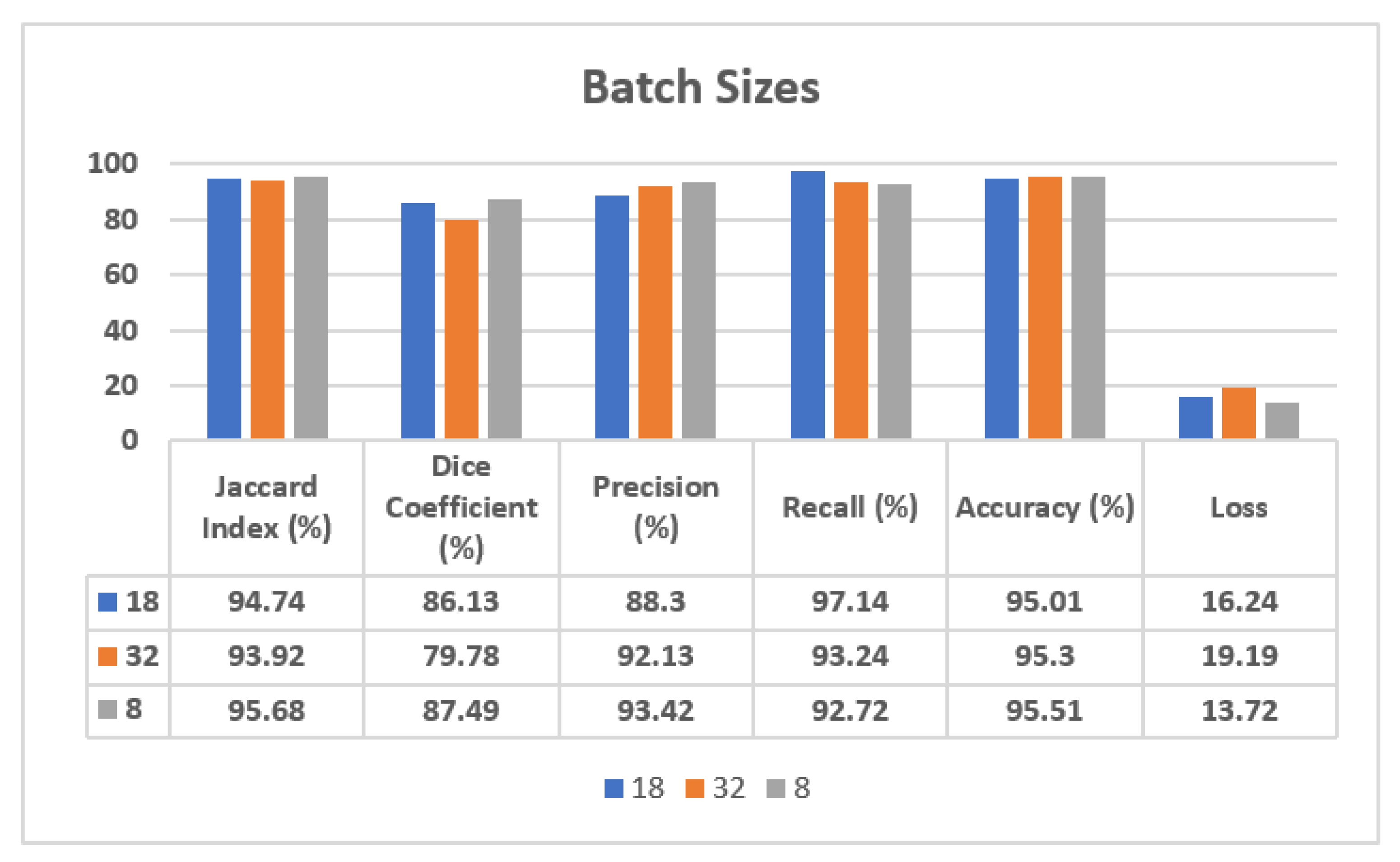
| 8 | 95.68 | 87.49 | 93.42 | 92.72 | 95.51 | 13.72 |
| 18 | 94.74 | 86.13 | 88.30 | 97.14 | 95.01 | 16.24 |
| 32 | 93.92 | 79.78 | 92.13 | 93.24 | 95.30 | 19.19 |
| Training Dataset | ||||||
|---|---|---|---|---|---|---|
| Epochs | Jaccard Index (%) | Dice Coefficient (%) | Precision (%) | Recall (%) | Accuracy (%) | Loss |
| 25 | 88.69 | 73.72 | 81.72 | 93.69 | 91.58 | 27.71 |
| 50 | 93.51 | 79.81 | 98.74 | 81.03 | 93.62 | 18.99 |
| 75 | 97.66 | 90.79 | 95.95 | 96.89 | 97.79 | 7.79 |
| 100 | 59.97 | 53.07 | 37.62 | 96.75 | 47.37 | 164.86 |
| Testing Dataset | ||||||
| Jaccard Index (%) | Dice Coefficient (%) | Precision (%) | Recall (%) | Accuracy (%) | Loss | |
| 25 | 89.72 | 72.95 | 80.05 | 94.58 | 91.64 | 27.60 |
| 50 | 93.10 | 78.97 | 96.55 | 81.10 | 93.35 | 19.44 |
| 75 | 95.57 | 87.41 | 90.62 | 95.23 | 95.47 | 13.78 |
| 100 | 57.38 | 50.65 | 35.46 | 96.86 | 43.25 | 181.64 |
| Validation Dataset | ||||||
| Jaccard Index (%) | Dice Coefficient (%) | Precision (%) | Recall (%) | Accuracy (%) | Loss | |
| 25 | 89.56 | 73.90 | 81.96 | 92.34 | 91.00 | 28.17 |
| 50 | 92.10 | 77.69 | 97.31 | 77.58 | 91.72 | 23.37 |
| 75 | 96.35 | 89.01 | 93.56 | 94.91 | 96.27 | 11.56 |
| 100 | 59.78 | 53.26 | 37.58 | 96.73 | 47.15 | 165.86 |
| Ref | Technique Used | Dataset | Performance Parameters |
|---|---|---|---|
| Yuan et al. [10] | 19-layer Deep Convolution Network | ISBI-2016 | Jaccard Coefficient = 0.963 |
| PH2 | |||
| Yuan et al. [11] | Convolutional-Deconvolutional neural Network | ISBI-2017 | Jaccard Coefficient = 0.784 |
| Hang Li et al. [28] | Dense Deconvolutional Network | ISBI-2016 | Jaccard Coefficient = 0.870 |
| ISBI-2017 | Jaccard Coefficient = 0.765 | ||
| Yu et al. [29] | Convolution Network | ISBI-2016 | Accuracy = 0.8654 |
| ISBI-2017 | |||
| Khan et al. [30] | Convolution Network | ISIC | Accuracy = 0.968 |
| PH2 | Accuracy = 0.921 | ||
| Proposed Model | Modified U-Net | PH2 | Jaccard Coefficient = 0.976 |
| Architecture | Accuracy = 0.977 |
Publisher’s Note: MDPI stays neutral with regard to jurisdictional claims in published maps and institutional affiliations. |
© 2022 by the authors. Licensee MDPI, Basel, Switzerland. This article is an open access article distributed under the terms and conditions of the Creative Commons Attribution (CC BY) license (https://creativecommons.org/licenses/by/4.0/).
Share and Cite
Anand, V.; Gupta, S.; Koundal, D.; Nayak, S.R.; Barsocchi, P.; Bhoi, A.K. Modified U-NET Architecture for Segmentation of Skin Lesion. Sensors 2022, 22, 867. https://doi.org/10.3390/s22030867
Anand V, Gupta S, Koundal D, Nayak SR, Barsocchi P, Bhoi AK. Modified U-NET Architecture for Segmentation of Skin Lesion. Sensors. 2022; 22(3):867. https://doi.org/10.3390/s22030867
Chicago/Turabian StyleAnand, Vatsala, Sheifali Gupta, Deepika Koundal, Soumya Ranjan Nayak, Paolo Barsocchi, and Akash Kumar Bhoi. 2022. "Modified U-NET Architecture for Segmentation of Skin Lesion" Sensors 22, no. 3: 867. https://doi.org/10.3390/s22030867