
Probabilistic Modeling of Motion Blur for Time-of-Flight Sensors


Abstract
:1. Introduction
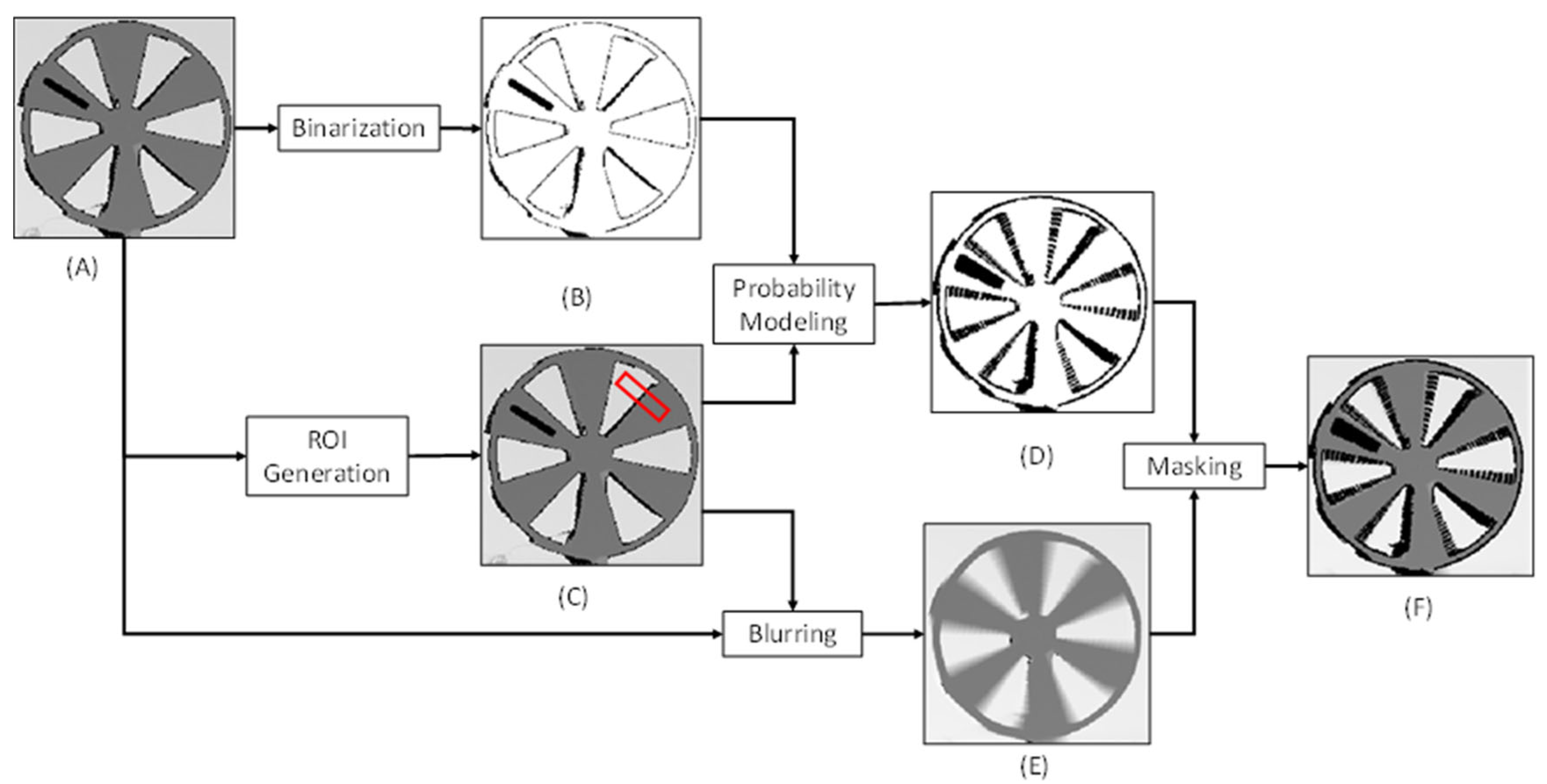
2. Methodology
2.1. ROI Generation
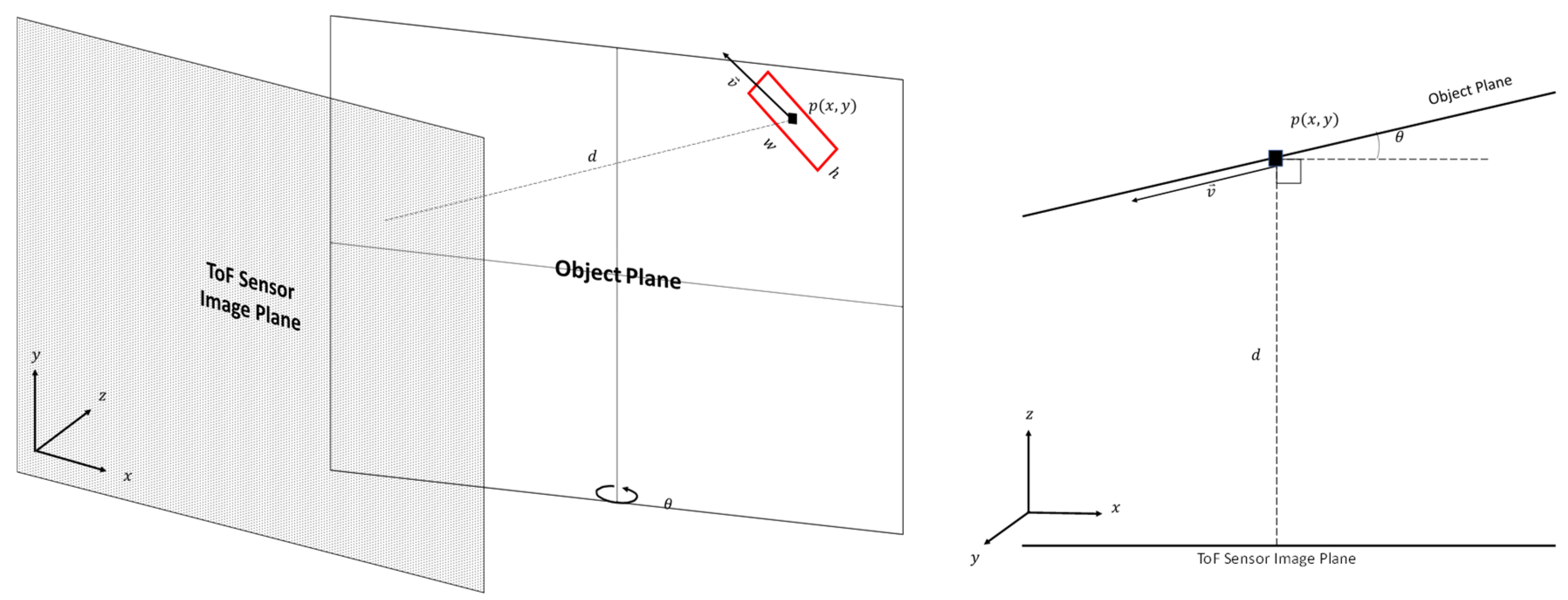
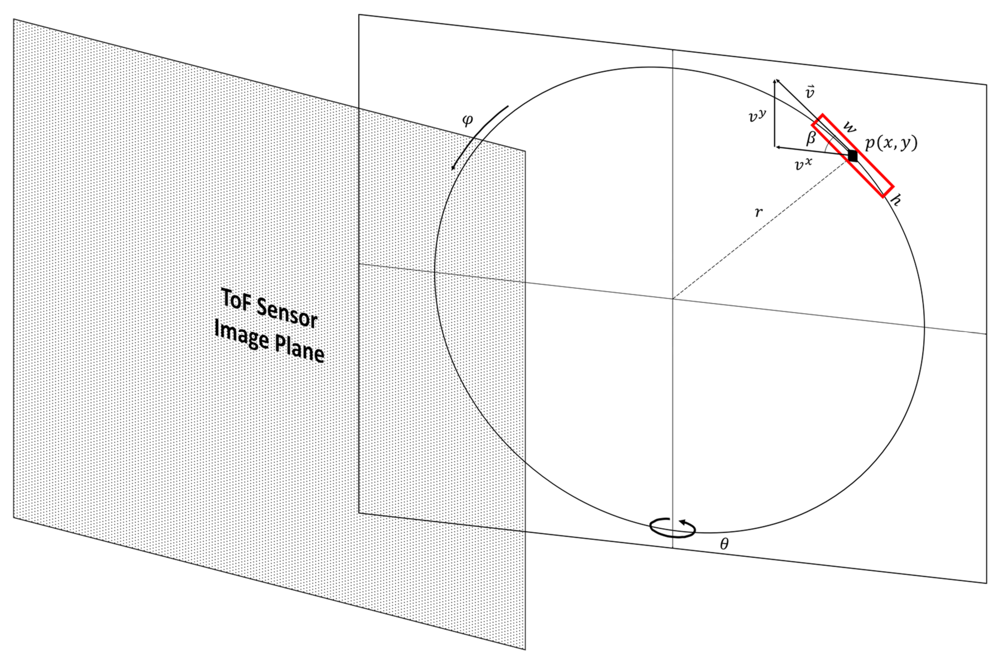
2.1.1. Radial Velocity
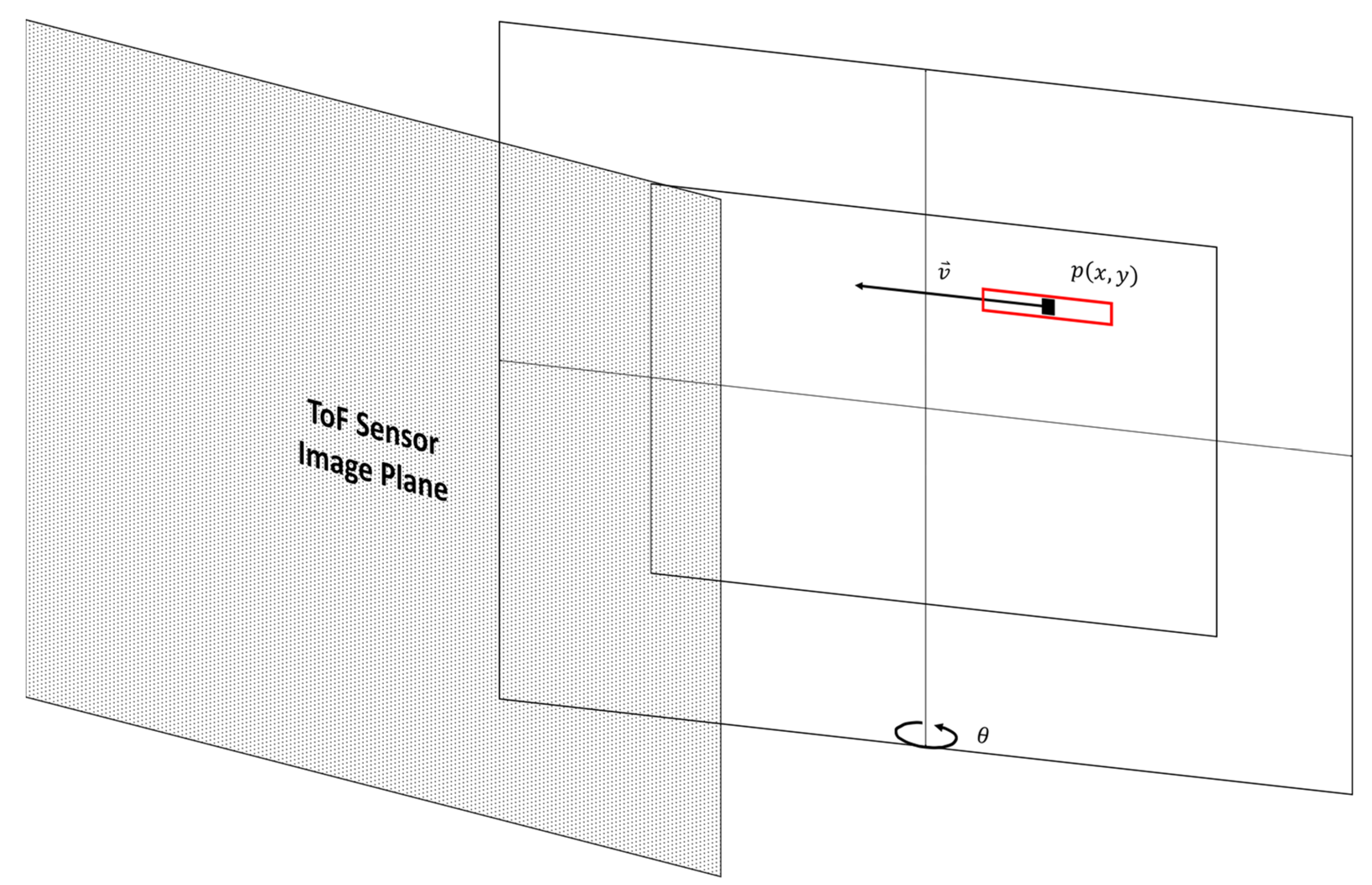
2.1.2. Linear Velocity
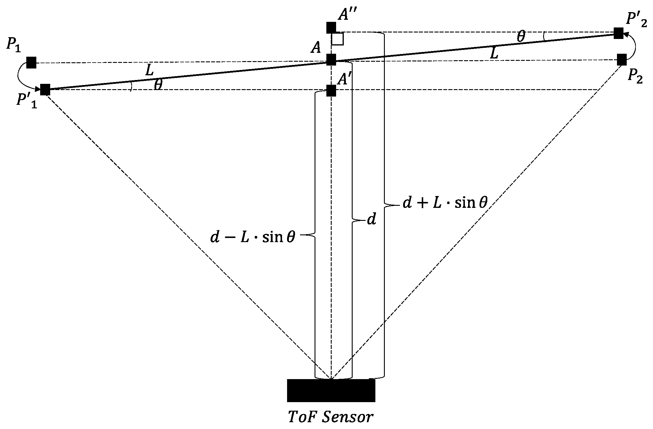
2.1.3. Perspective Distortion Function
2.2. Blurring the Depth Map
2.3. Probability Modeling
3. Experiments
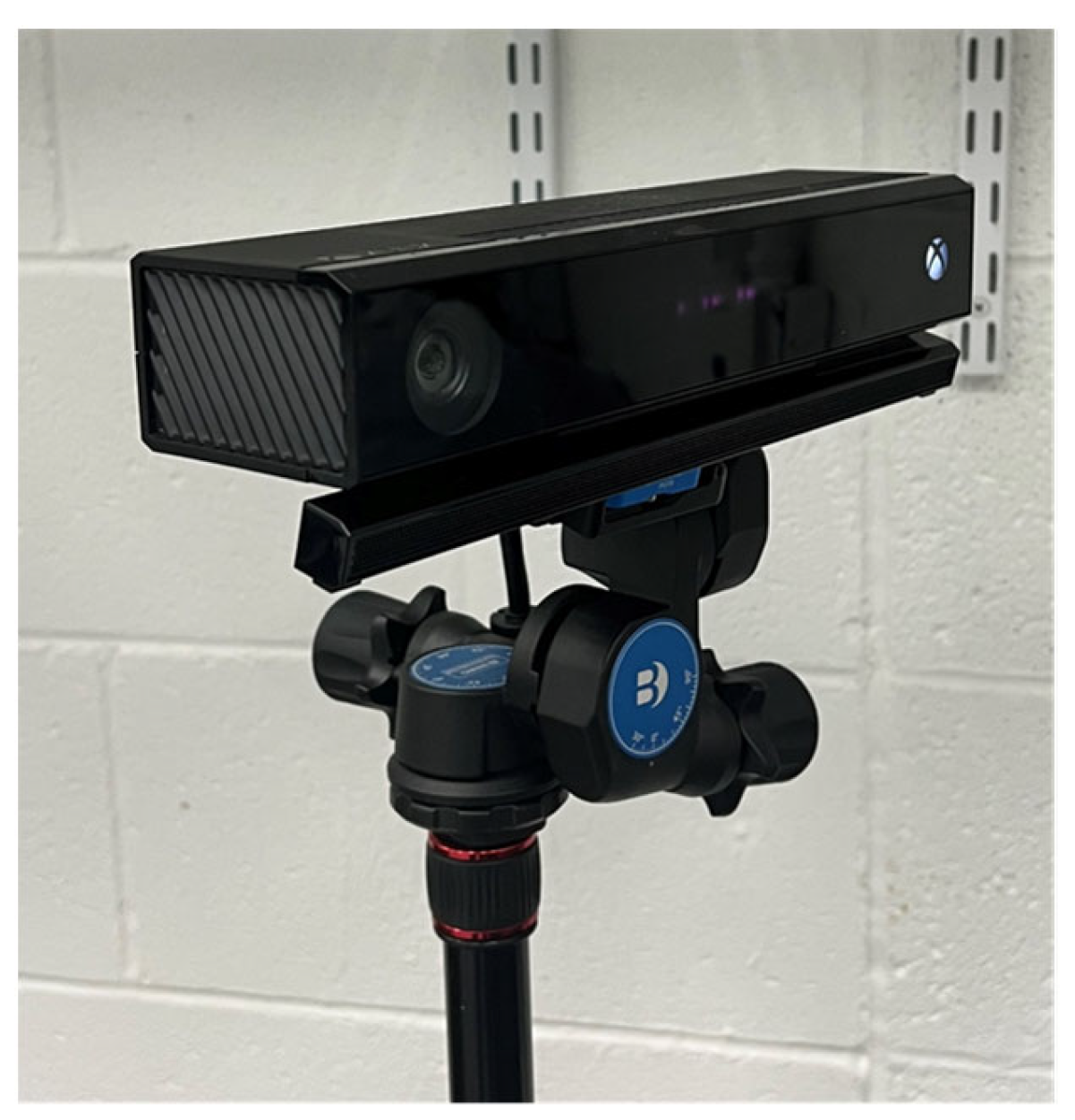
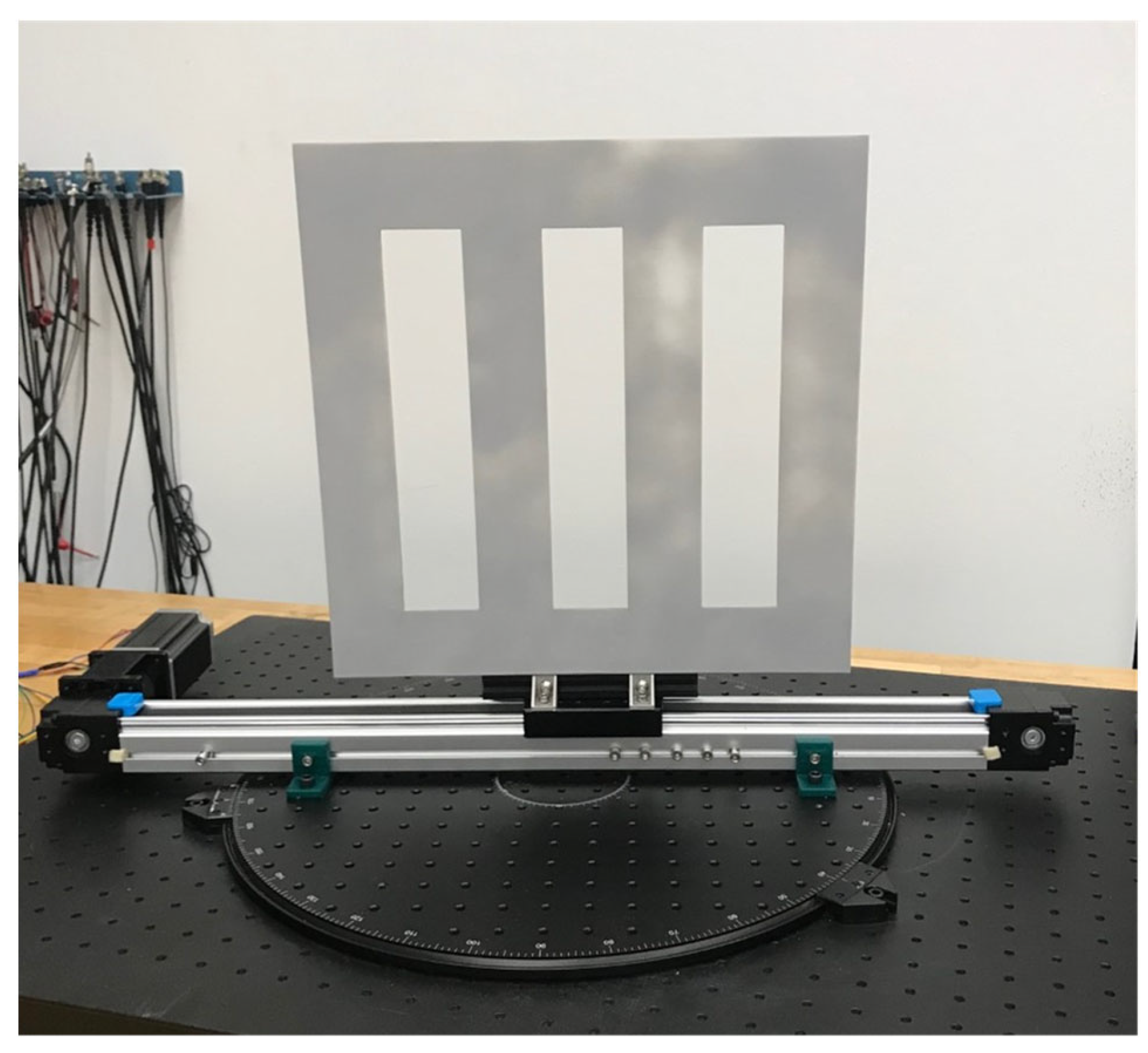
3.1. Hardware Configuration
3.2. Verification Results for the Probabilistic Model Assumptions
3.3. Performance Metrics
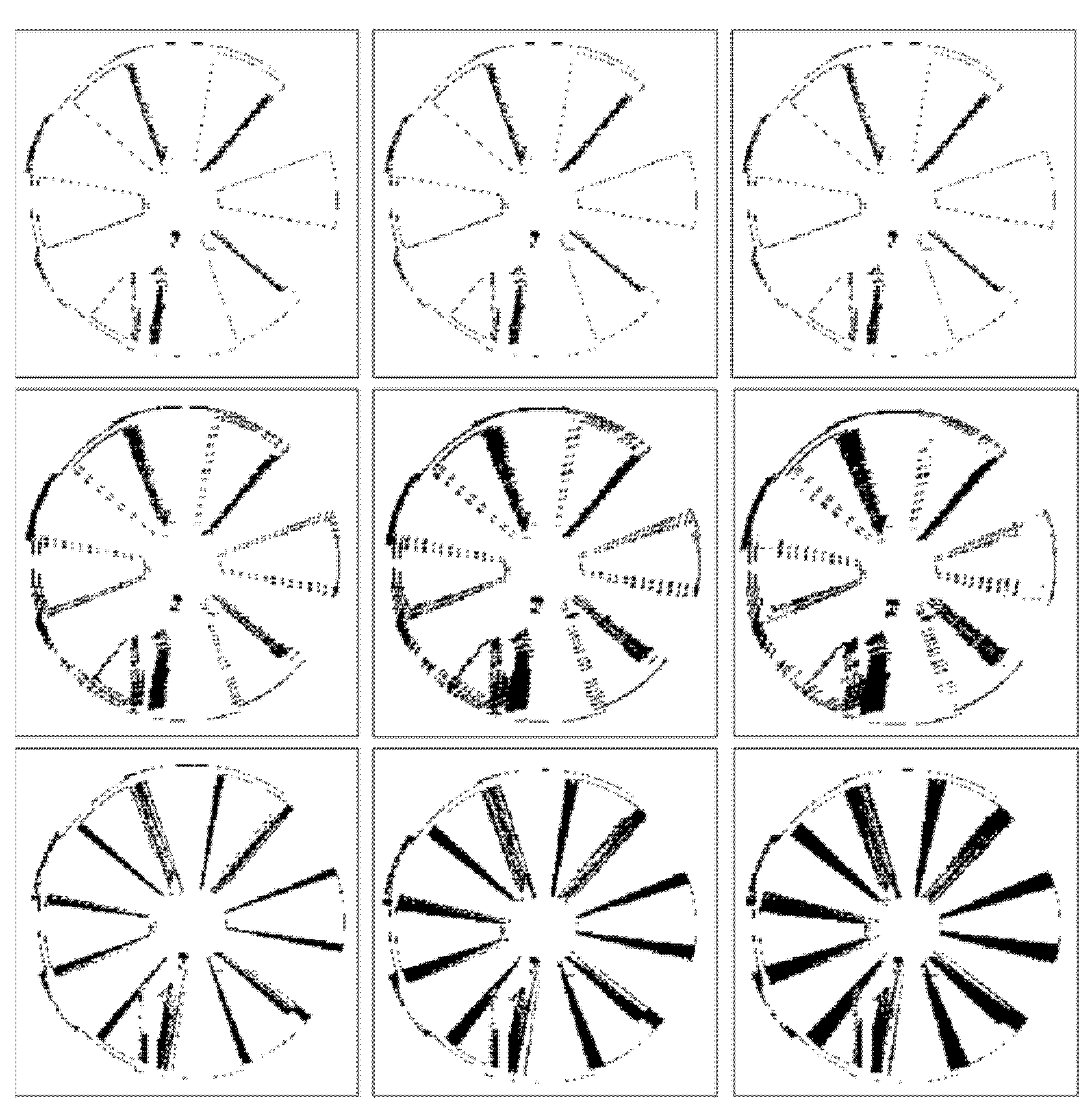
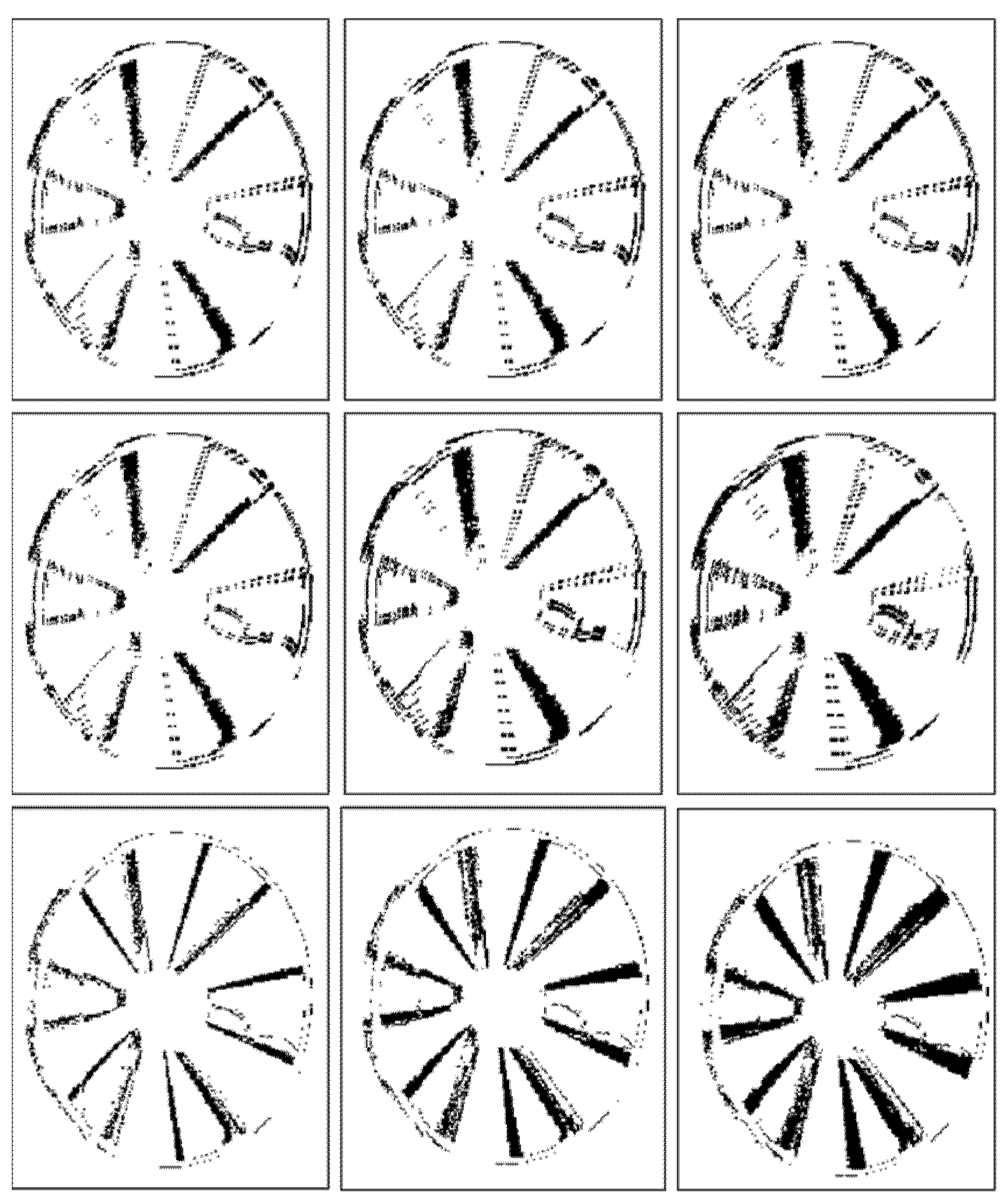
3.4. Radial Motion Blur Experiments
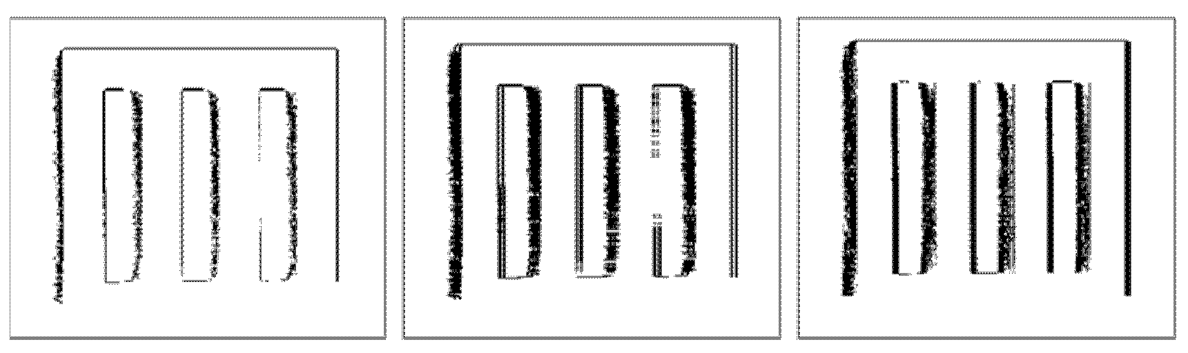
3.5. Linear Motion Blur Experimental Results
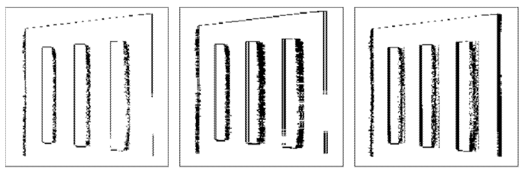
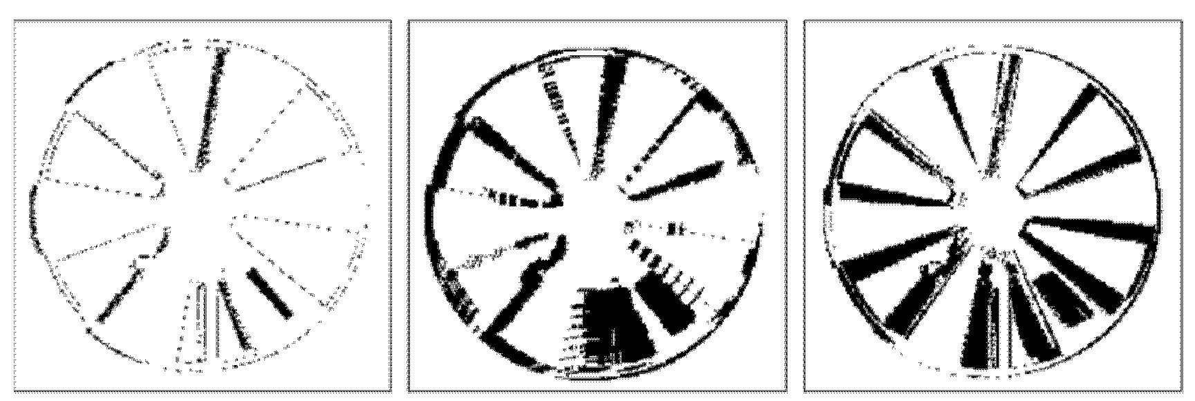
3.6. Combined Radial and Linear Motion Blur Experimental Results
3.7. Validating Synthetic Motion Generating Framework Using Other ToF Sensors
4. Conclusions
Author Contributions
Funding
Institutional Review Board Statement
Informed Consent Statement
Data Availability Statement
Acknowledgments
Conflicts of Interest
References
- Page, D.L.; Fougerolle, Y.; Koschan, A.F.; Gribok, A.; Abidi, M.A.; Gorsich, D.J.; Gerhart, G.R. SAFER vehicle inspection: A multimodal robotic sensing platform. In Unmanned Ground Vehicle Technology VI, Proceedings of the Defense and Security, Orlando, FL, USA, 12–16 April 2004; SPIE: Bellingham, WA, USA, 2004; Volume 5422, pp. 549–561. [Google Scholar] [CrossRef]
- Chen, C.; Yang, B.; Song, S.; Tian, M.; Li, J.; Dai, W.; Fang, L. Calibrate Multiple Consumer RGB-D Cameras for Low-Cost and Efficient 3D Indoor Mapping. Remote Sens. 2018, 10, 328. [Google Scholar] [CrossRef] [Green Version]
- Zhang, X.; Rajan, D.; Story, B. Concrete crack detection using context-aware deep semantic segmentation network. Comput. Civ. Infrastruct. Eng. 2019, 34, 951–971. [Google Scholar] [CrossRef]
- Zhang, X.; Zeinali, Y.; Story, B.A.; Rajan, D. Measurement of Three-Dimensional Structural Displacement Using a Hybrid Inertial Vision-Based System. Sensors 2019, 19, 4083. [Google Scholar] [CrossRef] [PubMed] [Green Version]
- Guo, F.; Qian, Y.; Shi, Y. Real-time railroad track components inspection based on the improved YOLOv4 framework. Autom. Constr. 2021, 125, 103596. [Google Scholar] [CrossRef]
- Guo, F.; Qian, Y.; Wu, Y.; Leng, Z.; Yu, H. Automatic railroad track components inspection using real-time instance segmentation. Comput. Civ. Infrastruct. Eng. 2021, 36, 362–377. [Google Scholar] [CrossRef]
- Paredes, J.A.; Álvarez, F.J.; Aguilera, T.; Villadangos, J.M. 3D indoor positioning of UAVs with spread spectrum ultrasound and time-of-flight cameras. Sensors 2018, 18, 89. [Google Scholar] [CrossRef] [Green Version]
- Mentasti, S.; Pedersini, F. Controlling the Flight of a Drone and Its Camera for 3D Reconstruction of Large Objects. Sensors 2019, 19, 2333. [Google Scholar] [CrossRef] [Green Version]
- Jin, Y.-H.; Ko, K.-W.; Lee, W.-H. An Indoor Location-Based Positioning System Using Stereo Vision with the Drone Camera. Mob. Inf. Syst. 2018, 2018, 5160543. [Google Scholar] [CrossRef] [Green Version]
- Pascoal, R.; Santos, V.; Premebida, C.; Nunes, U. Simultaneous Segmentation and Superquadrics Fitting in Laser-Range Data. IEEE Trans. Veh. Technol. 2014, 64, 441–452. [Google Scholar] [CrossRef]
- Shen, S.; Mulgaonkar, Y.; Michael, N.; Kumar, V. Multi-Sensor Fusion for Robust Autonomous Flight in Indoor and Outdoor Environments with a Rotorcraft MAV. In Proceedings of the 2014 IEEE International Conference on Robotics and Automation (ICRA), Hong Kong, China, 31 May–7 June 2014; pp. 4974–4981. [Google Scholar]
- Chiodini, S.; Giubilato, R.; Pertile, M.; Debei, S. Retrieving Scale on Monocular Visual Odometry Using Low-Resolution Range Sensors. IEEE Trans. Instrum. Meas. 2020, 69, 5875–5889. [Google Scholar] [CrossRef]
- Zhang, X.; Story, B.; Rajan, D. Night Time Vehicle Detection and Tracking by Fusing Vehicle Parts from Multiple Cameras. IEEE Trans. Intell. Transp. Syst. 2021, 1–21. [Google Scholar] [CrossRef]
- Zhang, X.; Story, B.; Rajan, D. Night Time Vehicle Detection and Tracking by Fusing Sensor Cues from Autonomous Vehicles. In Proceedings of the 2020 IEEE 91st Vehicular Technology Conference (VTC2020-Spring), Antwerp, Belgium, 25–28 May 2020; pp. 1–7. [Google Scholar]
- Wu, H.; Zhang, X.; Story, B.; Rajan, D. Accurate Vehicle Detection Using Multi-Camera Data Fusion and Machine Learning. In Proceedings of the 2019 IEEE International Conference on Acoustics, Speech and Signal Processing (ICASSP), Brighton, UK, 12–17 May 2019; pp. 3767–3771. [Google Scholar]
- Correll, N.; Bekris, K.E.; Berenson, D.; Brock, O.; Causo, A.; Hauser, K.; Okada, K.; Rodriguez, A.; Romano, J.M.; Wurman, P.R. Analysis and Observations from the First Amazon Picking Challenge. IEEE Trans. Autom. Sci. Eng. 2016, 15, 172–188. [Google Scholar] [CrossRef]
- Corbato, C.H.; Bharatheesha, M.; Van Egmond, J.; Ju, J.; Wisse, M. Integrating Different Levels of Automation: Lessons from Winning the Amazon Robotics Challenge 2016. IEEE Trans. Ind. Inform. 2018, 14, 4916–4926. [Google Scholar] [CrossRef] [Green Version]
- Pardi, T.; Poggiani, M.; Luberto, E.; Raugi, A.; Garabini, M.; Persichini, R.; Catalano, M.G.; Grioli, G.; Bonilla, M.; Bicchi, A. A Soft Robotics Approach to Autonomous Warehouse Picking. In Advances on Robotic Item Picking; Springer: Cham, Switzerland, 2020; pp. 23–35. [Google Scholar]
- Lindner, M.; Kolb, A. Compensation of Motion Artifacts for Time-of-Flight Cameras. In Workshop on Dynamic 3D Imaging; Springer: Berlin/Heidelberg, Germany, 2009; pp. 16–27. [Google Scholar]
- Gonzalez, R.C.; Woods, R.E. Digital Image Processing, 4th ed.; Pearson: Upper Saddle River, NJ, USA, 2018. [Google Scholar]
- Gonzalez, R.C.; Woods, R.E.; Eddins, S. Digital Image Processing Using MATLAB, 3rd ed.; Gatesmark: New York, NY, USA, 2020. [Google Scholar]
- Brooks, T.; Barron, J.T. Learning to Synthesize Motion Blur. In Proceedings of the 2019 IEEE/CVF Conference on Computer Vision and Pattern Recognition (CVPR), Long Beach, CA, USA, 15–20 June 2019; pp. 6840–6848. [Google Scholar]
- Leimkühler, T.; Seidel, H.-P.; Ritschel, T. Laplacian kernel splatting for efficient depth-of-field and motion blur synthesis or reconstruction. ACM Trans. Graph. 2018, 37, 1–11. [Google Scholar] [CrossRef] [Green Version]
- Guo, Q.; Juefei-Xu, F.; Xie, X.; Ma, L.; Wang, J.; Feng, W.; Liu, Y. Abba: Saliency-regularized motion-based adversarial blur attack. arXiv 2020, arXiv:2002.03500. [Google Scholar]
- Sun, J.; Cao, W.; Xu, Z.; Ponce, J. Learning a convolutional neural network for non-uniform motion blur removal. In Proceedings of the 2015 IEEE Conference on Computer Vision and Pattern Recognition (CVPR), Boston, MA, USA, 7–12 June 2015; pp. 769–777. [Google Scholar]
- Gong, D.; Yang, J.; Liu, L.; Zhang, Y.; Reid, I.; Shen, C.; van den Hengel, A.; Shi, Q. From Motion Blur to Motion Flow: A Deep Learning Solution for Removing Heterogeneous Motion Blur. In Proceedings of the 2017 IEEE Conference on Computer Vision and Pattern Recognition (CVPR), Honolulu, HI, USA, 21–26 July 2017; pp. 2319–2328. [Google Scholar]
- Noroozi, M.; Chandramouli, P.; Favaro, P. Motion Deblurring in the Wild. In Proceedings of the German Conference on Pattern Recognition (GCPR), Basel, Switzerland, 13–15 September 2017; Volume 10496, pp. 65–77. [Google Scholar]
- Kupyn, O.; Budzan, V.; Mykhailych, M.; Mishkin, D.; Matas, J. DeblurGAN: Blind Motion Deblurring Using Conditional Adversarial Networks. In Proceedings of the 2018 IEEE/CVF Conference on Computer Vision and Pattern Recognition (CVPR), Salt Lake City, UT, USA, 18–23 June 2018; pp. 8183–8192. [Google Scholar] [CrossRef] [Green Version]
- Wieschollek, P.; Hirsch, M.; Scholkopf, B.; Lensch, H.P. Learning Blind Motion Deblurring. In Proceedings of the 2017 IEEE International Conference on Computer Vision (ICCV), Venice, Italy, 22–29 October 2017; pp. 231–240. [Google Scholar]
- Chakrabarti, A. A Neural Approach to Blind Motion Deblurring. In Proceedings of the European Conference on Computer Vision (ECCV), Amsterdam, The Netherlands, 8–16 October 2016; pp. 221–235. [Google Scholar]
- Mutto, C.D.; Zanuttigh, P.; Cortelazzo, G.M. Time-of-Flight Cameras and Microsoft Kinect™; Springer Science and Business Media: New York, NY, USA, 2012. [Google Scholar]
- Hansard, M.; Lee, S.; Choi, O.; Horaud, R. Time of Flight Cameras: Principles, Methods, and Applications; Springer Science and Business Media: New York, NY, USA, 2012. [Google Scholar]
- Lee, S.; Kang, B.; Kim, J.D.; Kim, C.Y. Motion blur-free time-of-flight range sensor. In Proceedings of the SPIE 8298 Sensors, Cameras, and Systems for Industrial and Scientific Applications XIII, 82980U, Burlingame, CA, USA, 22–26 January 2012; Volume 8298. [Google Scholar] [CrossRef]
- Hussmann, S.; Hermanski, A.; Edeler, T. Real-Time Motion Artifact Suppression in TOF Camera Systems. IEEE Trans. Instrum. Meas. 2011, 60, 1682–1690. [Google Scholar] [CrossRef]
- Sarbolandi, H.; Lefloch, D.; Kolb, A. Kinect range sensing: Structured-light versus Time-of-Flight Kinect. Comput. Vis. Image Underst. 2015, 139, 1–20. [Google Scholar] [CrossRef] [Green Version]
- Rodriguez, B.; Zhang, X.; Rajan, D. Synthetically Generating Motion Blur in a Depth Map from Time-of-Flight Sensors. In Proceedings of the 2021 17th International Conference on Machine Vision and Applications (MVA), Aichi, Japan, 25–27 July 2021; pp. 1–5. [Google Scholar]
- Wood, F.E. Similar-Perspective Triangles. Am. Math. Mon. 1929, 36, 67. [Google Scholar] [CrossRef]
- Xiao, F. CEQD: A Complex Mass Function to Predict Interference Effects. IEEE Trans. Cybern. 2021, 1–13. [Google Scholar] [CrossRef]
- Xiao, F. CaFtR: A Fuzzy Complex Event Processing Method. Int. J. Fuzzy Syst. 2021, 1–14. [Google Scholar] [CrossRef]
- Kolb, A.; Barth, E.; Koch, R.; Larsen, R. Time-of-Flight Cameras in Computer Graphics. Comput. Graph. Forum 2010, 29, 141–159. [Google Scholar] [CrossRef]
- Jiao, J.; Yuan, L.; Tang, W.; Deng, Z.; Wu, Q. A post-rectification approach of depth images of Kinect v2 for 3D reconstruction of indoor scenes. ISPRS Int. J. Geo-Inf. 2017, 6, 349. [Google Scholar] [CrossRef] [Green Version]
- OpenKinect. OpenKinect Project. Available online: https://openkinect.org/wiki/Main_Page (accessed on 25 November 2020).
- MATLAB, version 99.0. 1467703 (R2020b); The MathWorks Inc.: Natick, MA, USA, 2020.
- Cheng, A.; Harrison, H. Touch Projector. Available online: https://tinyurl.com/bx3pfsxt (accessed on 25 November 2020).
- Benro. Benro GD3WH 3-Way Geared Head. Available online: https://benrousa.com/benro-gd3wh-3-way-geared-head/ (accessed on 26 April 2021).
- DXL360/S V2 Digital Protractor User Guide. Available online: https://www.roeckle.com/WebRoot/Store13/Shops/62116134/5EB6/6EBD/9A39/4D35/9E28/0A0C/6D12/406A/DXL360S_v2-Dual_Axis_Digital_Protractors.pdf (accessed on 27 April 2021).
- Thorlabs. Large-Area Rotating Breadboard. Available online: https://www.thorlabs.com/newgrouppage9.cfm?objectgroup_ID=5087 (accessed on 26 April 2021).
- Stepper Online. Stepper Motor 17HS24-2104S. Available online: https://www.omc-stepperonline.com/download/17HS24-2104S.pdf (accessed on 28 January 2021).
- Sorotec. TB6600 Data Sheet. Available online: https://www.mcielectronics.cl/website_MCI/static/documents/TB6600_data_sheet.pdf (accessed on 11 December 2020).
- Arduino. Arduino Uno Rev3. Available online: https://docs.arduino.cc/resources/datasheets/A000066-datasheet.pdf (accessed on 11 December 2020).
- Stepper Online. Stepper Motor 23HS45-4204S. Available online: https://www.omc-stepperonline.com/download/23HS45-4204S.pdf (accessed on 12 April 2021).
- Stepper Online. User’s Manual for DM542T. Available online: https://www.omc-stepperonline.com/download/DM542T.pdf (accessed on 12 April 2021).
- Csurka, G.; Larlus, D.; Perronnin, F. What is a good evaluation measure for semantic segmentation? In Proceedings of the British Machine Vision Conference 2013, Bristol, UK, 9–13 September 2013; Volume 27, p. 10.5244. [Google Scholar] [CrossRef] [Green Version]
- Texas Instruments. OPT8241-QVGA-Resolution 3D Time-of-Flight (ToF) Sensor. Available online: https://tinyurl.com/y5g6n5xh (accessed on 11 May 2016).


| Symbol | Description |
|---|---|
| p(x, y) | The pixel of a depth map in Cartesian coordinates |
| d | The distance between the image plane of a ToF sensor and a point in the object plane |
| 𝜃 | The rotation angle between the motion of an object and the image plane of a ToF sensor |
| I | The initial depth map in 2D matrix of pixels with dimensions M × N |
| Ib | The binary depth map in 2D matrix of pixels with dimensions M × N |
| If | The blurred depth map in 2D matrix of pixels with dimensions M × N |
| The velocity of a pixel at p(x, y) | |
| vx | The velocity component in the x-direction |
| vy | The velocity component in the y-direction |
| w | The ROI dimension tangential to the velocity of a pixel at p(x, y) |
| h | The ROI dimension orthogonal to the velocity of a pixel at p(x, y) |
| s(x, y) | The perspective distortion scaling function of a pixel at p(x, y) |
| β | The rotation angle of an ROI within a depth map |
| The angular motor velocity of a radial motion | |
| The linear motor velocity of a linear motion | |
| {n0, n1, …, nl} | The set of neighboring pixels within an ROI for a given pixel p(x, y) |
| pp | The initial probability of a given pixel p(x, y) having a value of zero |
| ε(sp, sni) | The potential function of the ith neighboring pixel to the given pixel p(x, y) |
| The predicted probability of a given pixel p(x, y) having a value of zero | |
| The predicted state of a given pixel p(x, y) having a value of one or zero in a binary depth map |
| Angle between the Sensor Plane and the Plane of Rotation of the Siemens Star | ||||
| Speed | 0 | 15 | 20 | 30 |
| 60 RPM | 0.1212 | 0.1140 | 0.1179 | 0.1170 |
| 100 RPM | 0.1884 | 0.1779 | 0.1789 | 0.1739 |
| 135 RPM | 0.2483 | 0.2355 | 0.2325 | 0.2261 |
| Angle between the Sensor Plane and the Plane of Rotation of the Siemens Star | ||||
| Speed | 0 | 15 | 20 | 30 |
| 60 RPM | 77.55% | 73.29% | 69.18% | 72.34% |
| 100 RPM | 74.45% | 75.07% | 70.28% | 72.22% |
| 135 RPM | 81.80% | 79.95% | 75.52% | 77.84% |
| Height Value: 1 Pixel | Rotation Angle | |||
| Speed | 0 | 15 | 20 | 30 |
| 60 RPM | 0.7873 | 0.7802 | 0.7866 | 0.7872 |
| 100 RPM | 0.7157 | 0.7091 | 0.7211 | 0.7337 |
| 135 RPM | 0.6401 | 0.6362 | 0.6593 | 0.6740 |
| Height value: 2 pixels | Rotation Angle | |||
| Speed | 0 | 15 | 20 | 30 |
| 60 RPM | 0.7757 | 0.7598 | 0.7579 | 0.7688 |
| 100 RPM | 0.6633 | 0.6604 | 0.6745 | 0.6991 |
| 135 RPM | 0.5808 | 0.5803 | 0.6075 | 0.6334 |
| Height value: 3 pixels | Rotation Angle | |||
| Speed | 0 | 15 | 20 | 30 |
| 60 RPM | 0.0170 | 0.0188 | 0.0229 | 0.0230 |
| 100 RPM | 0.0220 | 0.0248 | 0.0285 | 0.0282 |
| 135 RPM | 0.0312 | 0.0330 | 0.0389 | 0.0378 |
| Height value: 1 pixel | Rotation Angle | |||
| Speed | 0 | 15 | 20 | 30 |
| 60 RPM | 15.5832 | 16.3344 | 20.3076 | 19.7015 |
| 100 RPM | 19.06 | 21.3124 | 24.9468 | 24.7282 |
| 135 RPM | 27.5602 | 28.9867 | 35.3897 | 32.7857 |
| Height value: 2 pixels | Rotation Angle | |||
| Speed | 0 | 15 | 20 | 30 |
| 60 RPM | 16.5201 | 16.4827 | 19.6956 | 19.7207 |
| 100 RPM | 20.6372 | 22.3107 | 25.4945 | 25.3598 |
| 135 RPM | 28.6869 | 30.2006 | 35.8323 | 34.1595 |
| Height value: 3 pixels | Rotation Angle | |||
| Speed | 0 | 15 | 20 | 30 |
| 60 RPM | 16.5795 | 18.1961 | 22.7809 | 22.9275 |
| 100 RPM | 21.6180 | 24.0258 | 28.1812 | 28.1346 |
| 135 RPM | 30.6426 | 31.9231 | 38.7674 | 37.3976 |
| Height Value: 1 Pixel | Rotation Angle | |||
| Speed | 0 | 15 | 20 | 30 |
| 60 RPM | 0.0159 | 0.0168 | 0.02 | 0.0194 |
| 100 RPM | 0.0195 | 0.0217 | 0.0251 | 0.0245 |
| 135 RPM | 0.0281 | 0.0295 | 0.0354 | 0.0327 |
| Height value: 2 pixels | Rotation Angle | |||
| Speed | 0 | 15 | 20 | 30 |
| 60 RPM | 0.0170 | 0.0172 | 0.0202 | 0.0199 |
| 100 RPM | 0.0208 | 0.0230 | 0.0257 | 0.0255 |
| 135 RPM | 0.0291 | 0.0310 | 0.0358 | 0.0343 |
| Height value: 3 pixels | Rotation Angle | |||
| Speed | 0 | 15 | 20 | 30 |
| 60 RPM | 0.0170 | 0.0188 | 0.0229 | 0.0230 |
| 100 RPM | 0.0220 | 0.0248 | 0.0285 | 0.0282 |
| 135 RPM | 0.0312 | 0.0330 | 0.0389 | 0.0378 |
| Height Value: 1 Pixel | Rotation Angle | |||
| Metrics | 0 | 15 | 20 | 30 |
| BF Score | 0.8943 | 0.8498 | 0.8954 | 0.8778 |
| RMSE (mm) | 8.2291 | 7.4568 | 7.2266 | 6.9405 |
| RMSE-R | 0.0082 | 0.0072 | 0.0072 | 0.0066 |
| Height value: 2 pixels | Rotation Angle | |||
| Metrics | 0 | 15 | 20 | 30 |
| BF Score | 0.8292 | 0.7163 | 0.8493 | 0.8074 |
| RMSE (mm) | 8.2540 | 9.1342 | 8.0566 | 7.7380 |
| RMSE-R | 0.0082 | 0.0086 | 0.0081 | 0.0076 |
| Height value: 3 pixels | Rotation Angle | |||
| Metrics | 0 | 15 | 20 | 30 |
| BF Score | 0.8191 | 0.6592 | 0.8127 | 0.7752 |
| RMSE (mm) | 8.7983 | 9.3763 | 8.5384 | 8.1487 |
| RMSE-R | 0.0088 | 0.0089 | 0.0085 | 0.0081 |
| Height Value: 1 Pixel | Movement Direction | |
| Metrics | Left-to-Right | Right-to-Left |
| BF Score | 0.6092 | 0.6309 |
| RMSE (mm) | 106.0410 | 93.3467 |
| RMSE-R | 0.0733 | 0.0654 |
| Height value: 2 pixels | Movement Direction | |
| Metrics | Left-to-Right | Right-to-Left |
| BF Score | 0.5943 | 0.6131 |
| RMSE (mm) | 153.2062 | 148.2040 |
| RMSE-R | 0.0994 | 0.0965 |
| Height value: 3 pixels | Movement Direction | |
| Metrics | Left-to-Right | Right-to-Left |
| BF Score | 0.5790 | 0.6013 |
| RMSE (mm) | 197.8745 | 202.5617 |
| RMSE-R | 0.1254 | 0.1281 |
Publisher’s Note: MDPI stays neutral with regard to jurisdictional claims in published maps and institutional affiliations. |
© 2022 by the authors. Licensee MDPI, Basel, Switzerland. This article is an open access article distributed under the terms and conditions of the Creative Commons Attribution (CC BY) license (https://creativecommons.org/licenses/by/4.0/).
Share and Cite
Rodriguez, B.; Zhang, X.; Rajan, D. Probabilistic Modeling of Motion Blur for Time-of-Flight Sensors. Sensors 2022, 22, 1182. https://doi.org/10.3390/s22031182
Rodriguez B, Zhang X, Rajan D. Probabilistic Modeling of Motion Blur for Time-of-Flight Sensors. Sensors. 2022; 22(3):1182. https://doi.org/10.3390/s22031182
Chicago/Turabian StyleRodriguez, Bryan, Xinxiang Zhang, and Dinesh Rajan. 2022. "Probabilistic Modeling of Motion Blur for Time-of-Flight Sensors" Sensors 22, no. 3: 1182. https://doi.org/10.3390/s22031182