
Efficient WSN Node Placement by Coupling KNN Machine Learning for Signal Estimations and I-HBIA Metaheuristic Algorithm for Node Position Optimization


Abstract
:1. Introduction
2. Wireless Sensor Network Deployment
2.1. WSN Deployment Problematic
2.1.1. Classical Approaches
2.1.2. Modern Approaches
3. Proposed Approach
3.1. Coupling a Metaheuristic with a KNN Evalution Function
3.2. Signal Estimation with KNN Algorithm
3.3. Optimize Node Location with I-HBIA Metaheuristic
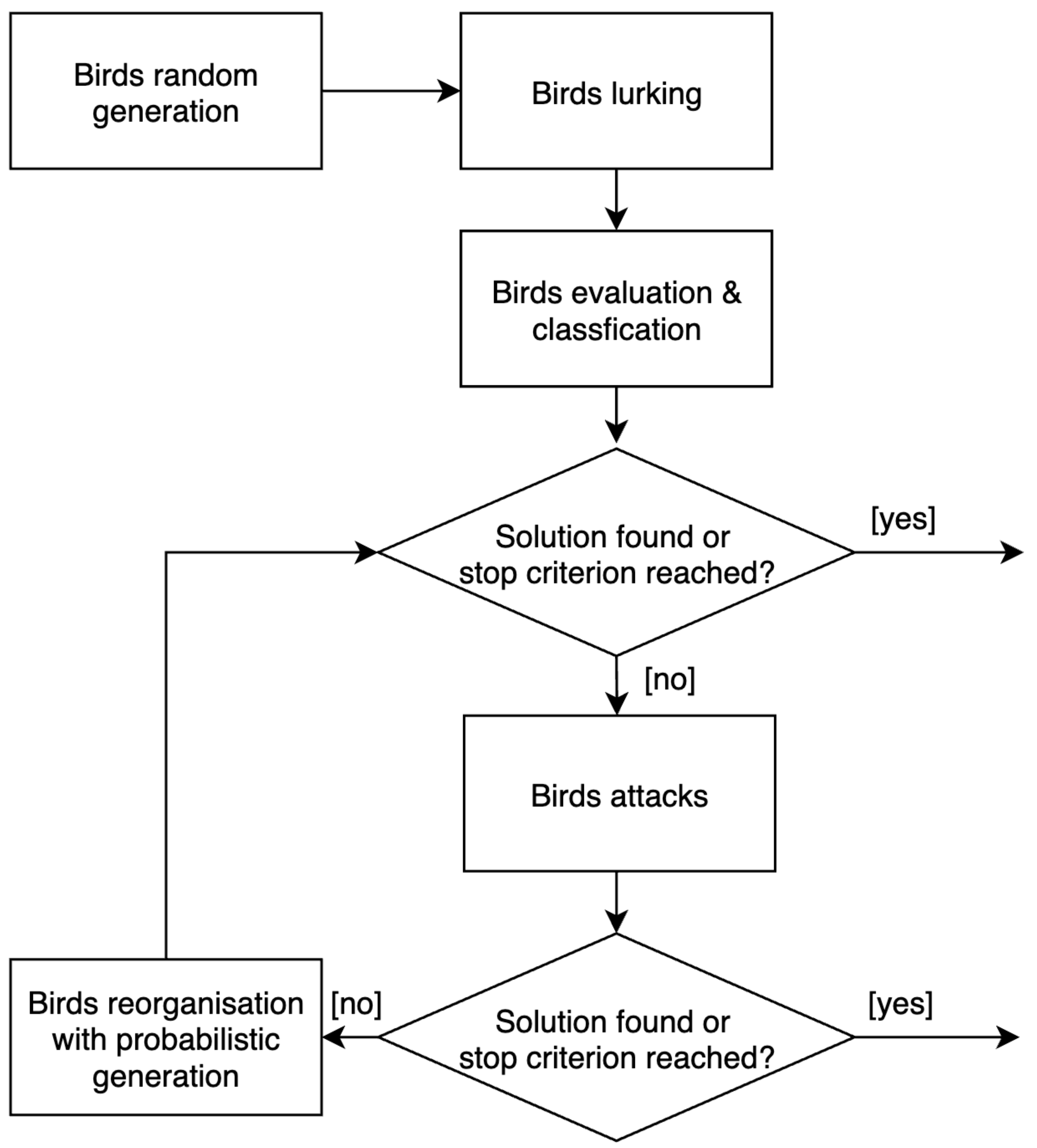
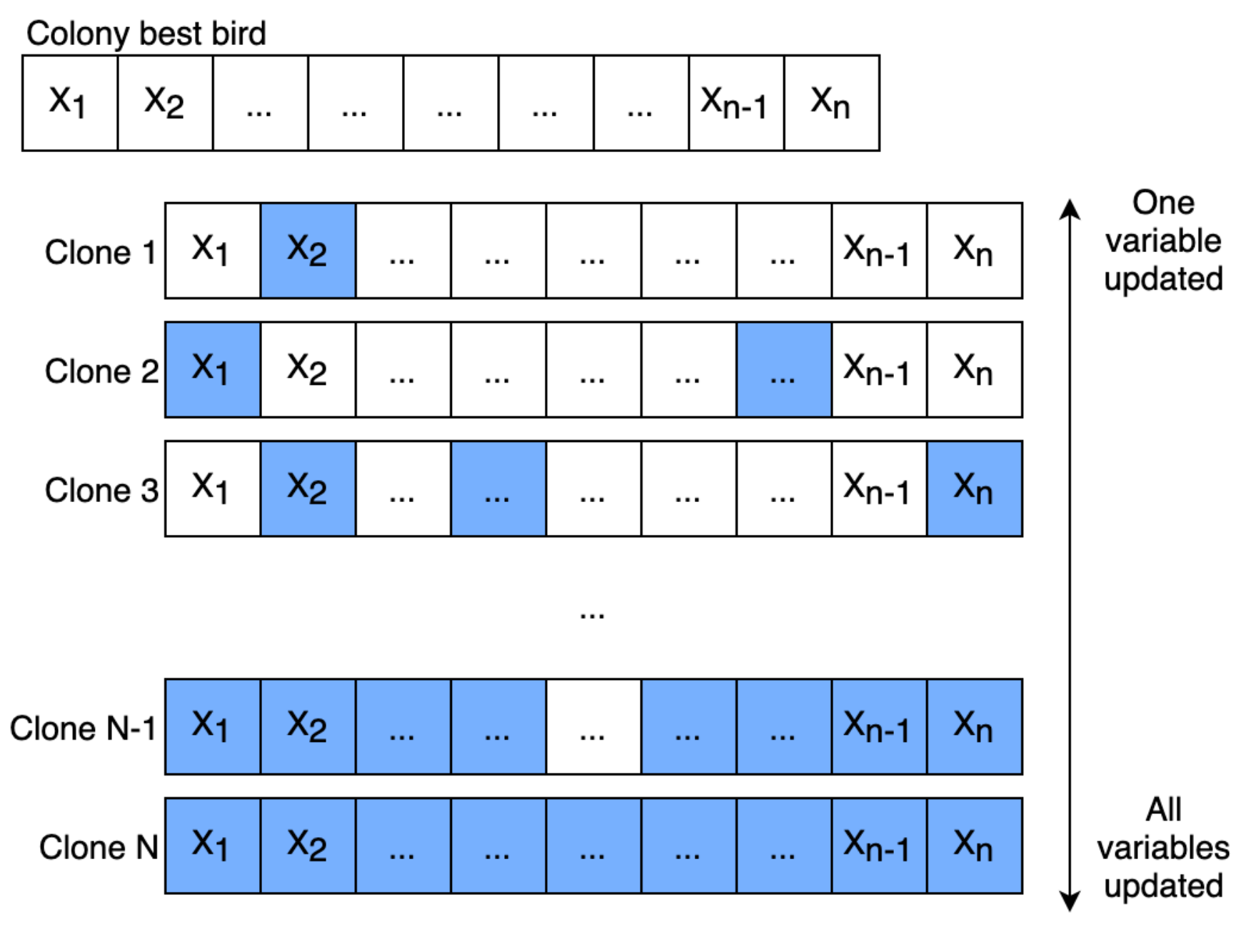
3.3.1. Canonical HBIA Algorithm
- This algorithm belongs to the family of P-Metaheuristics that base the optimization process on a set of solutions and are generally more efficient for optimization problems containing local minimums.
- This algorithm, in contrast to other metaheuristics, does not require many parameters. The only parameterization concerns the number of birds found in the colony. Moreover, the impact of the variations of this parameter on the results obtained remains marginal.
- This algorithm offers superior performance to many other metaheuristics on high dimensional problems. This aspect is particularly interesting for deploying sensor networks where the number of nodes and their positions can quickly become very large.
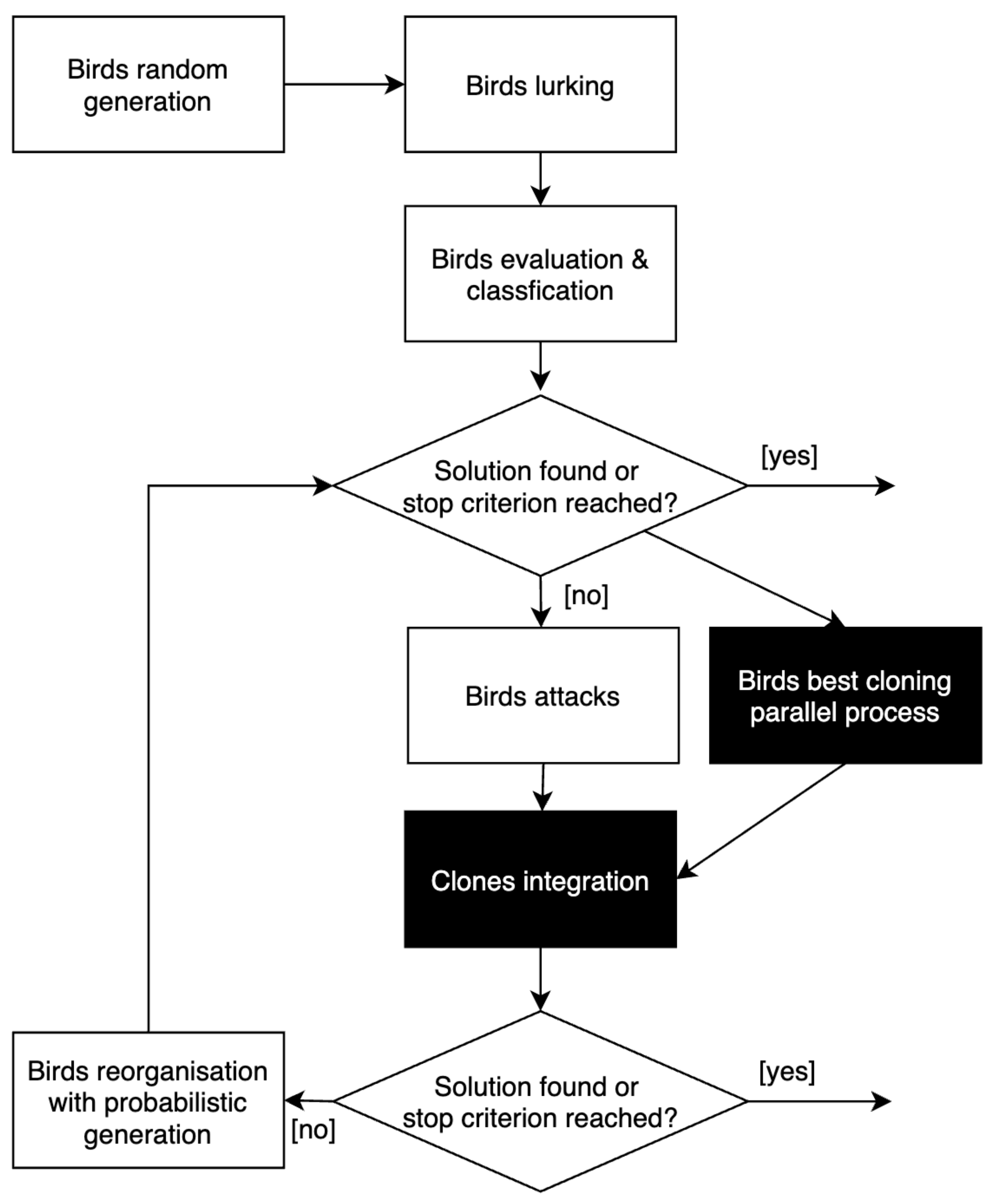
3.3.2. The I-HBIA Algorithm
4. Results
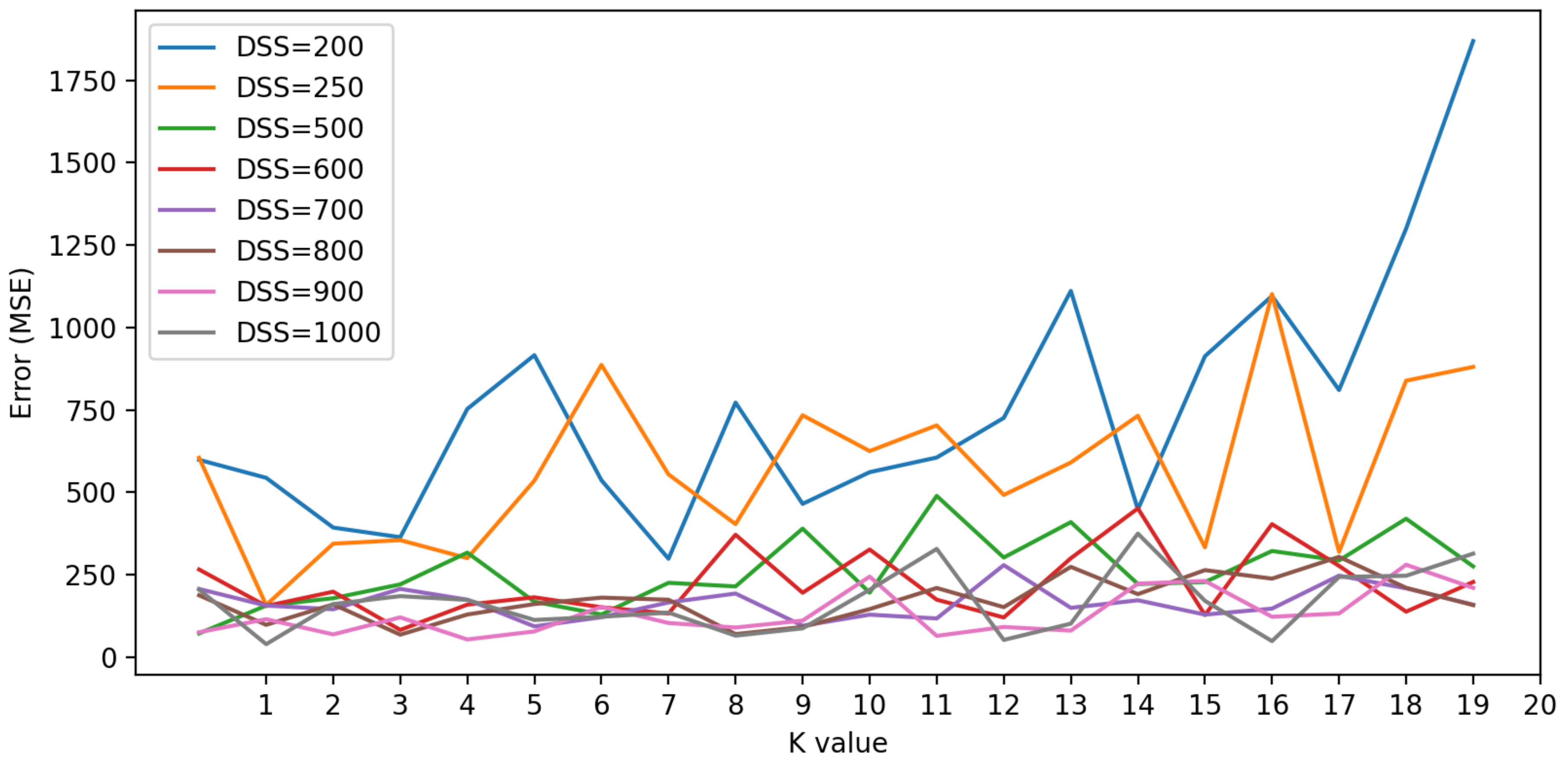
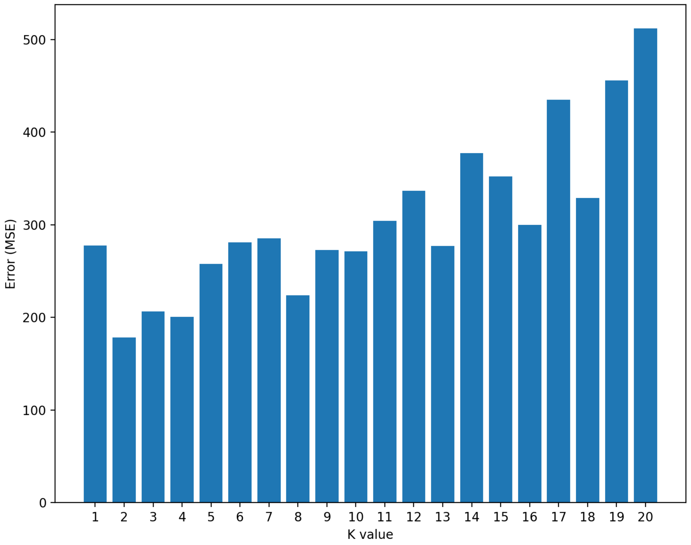
4.1. KNN Algorithm Parametrization
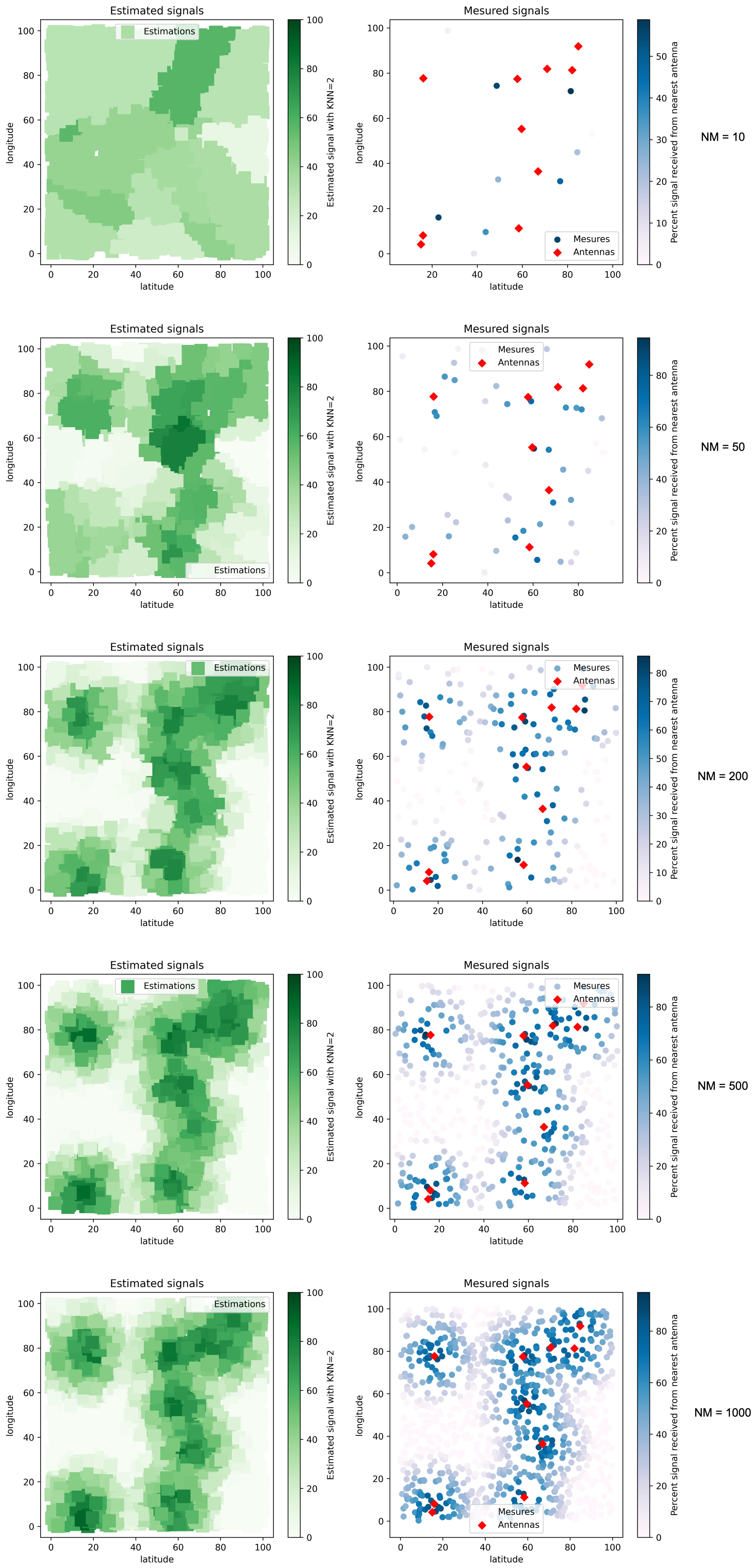
4.2. Signal Estimations on Maps
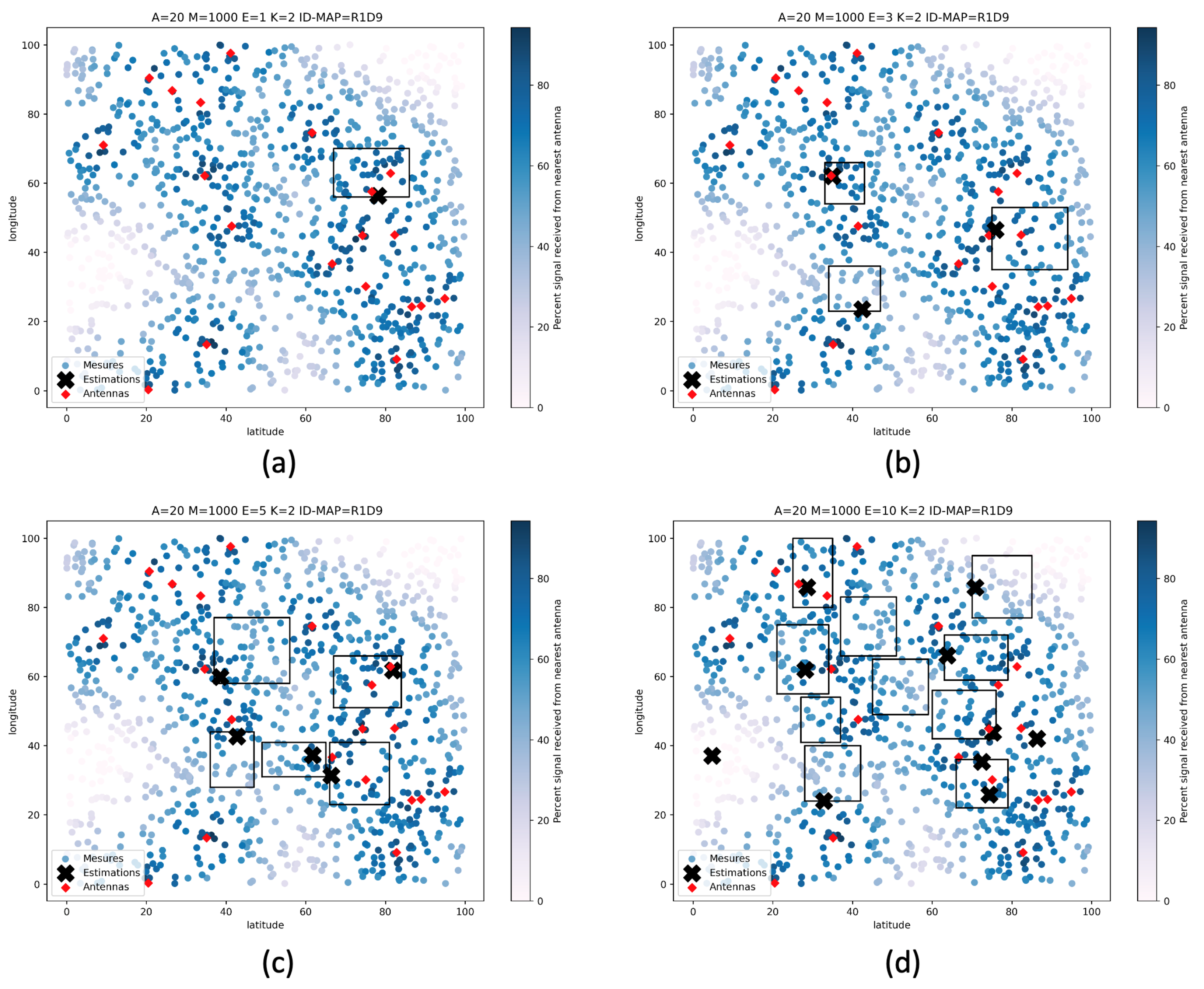
4.2.1. Signal Map without Obstacles
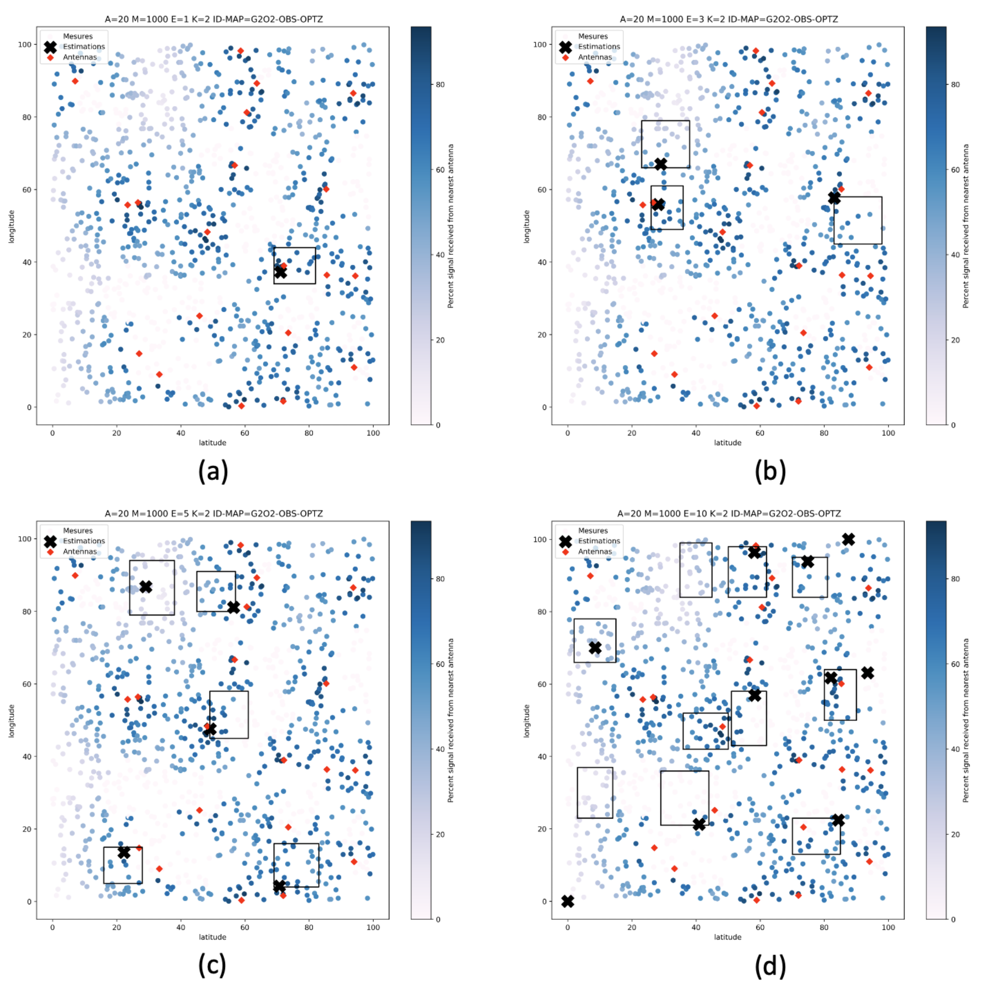
4.2.2. Signal Map with Obstacles
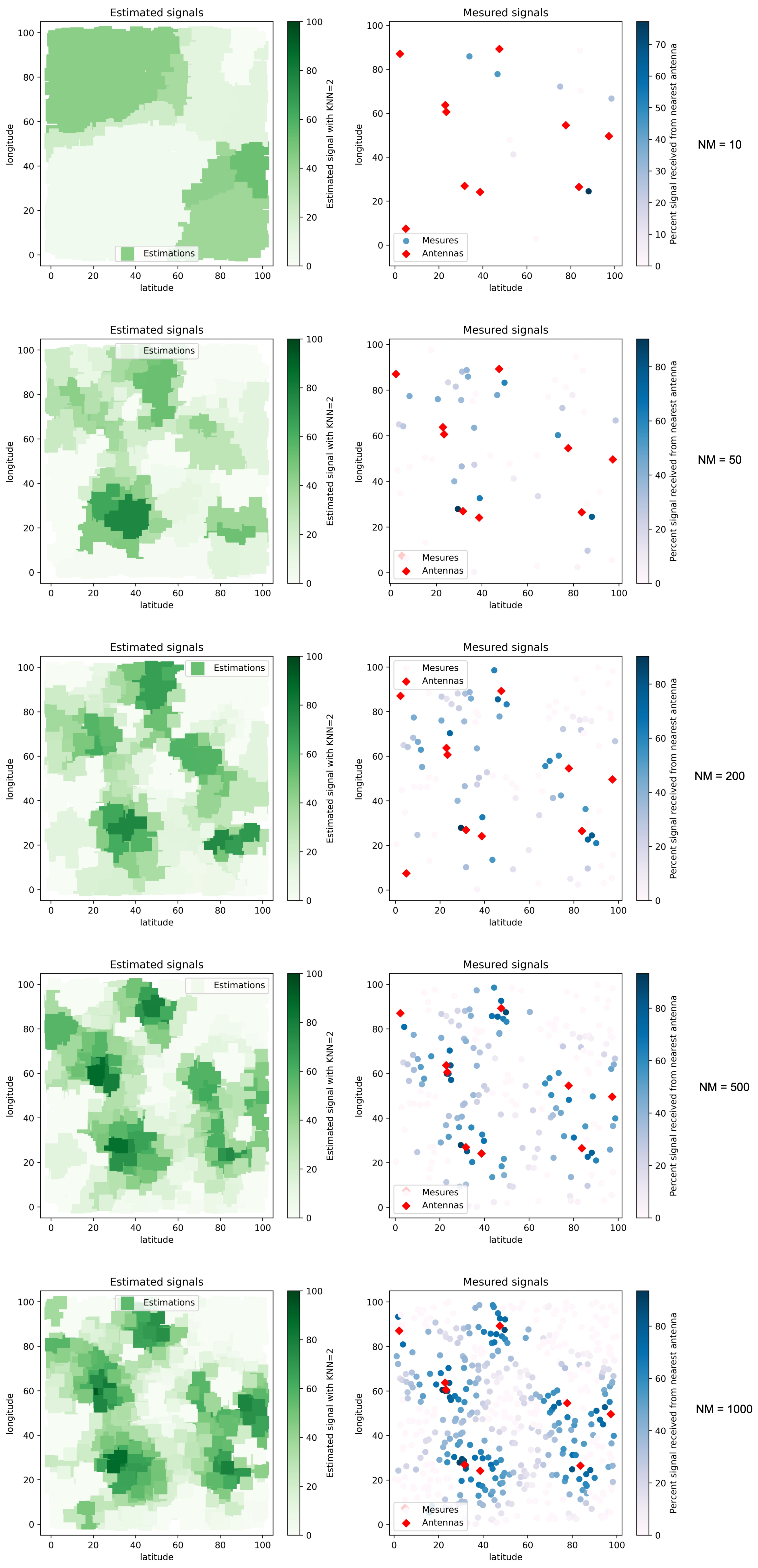
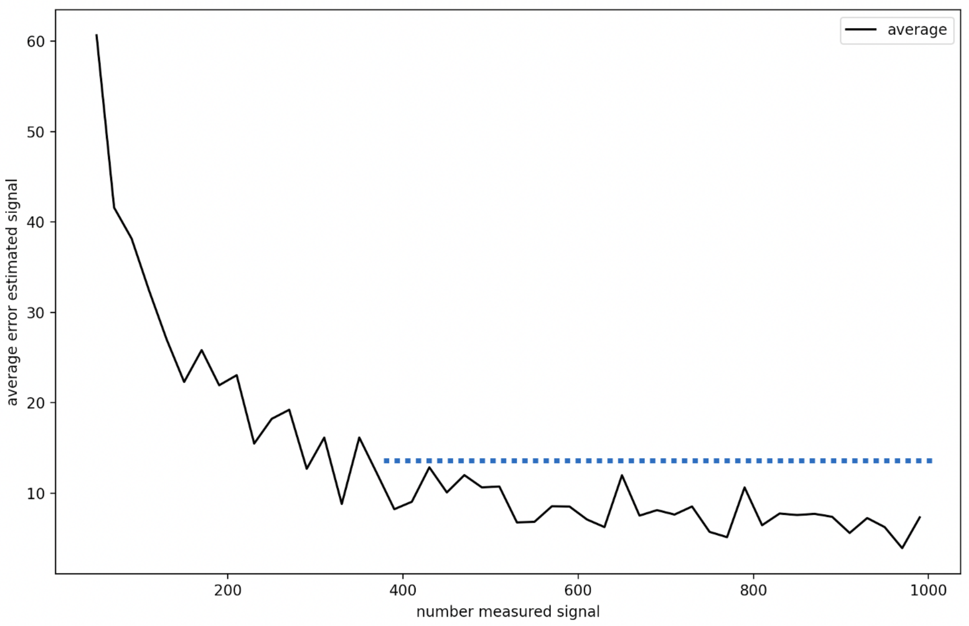
4.2.3. Influence of the Number of Measurements on the Quality of Predictions
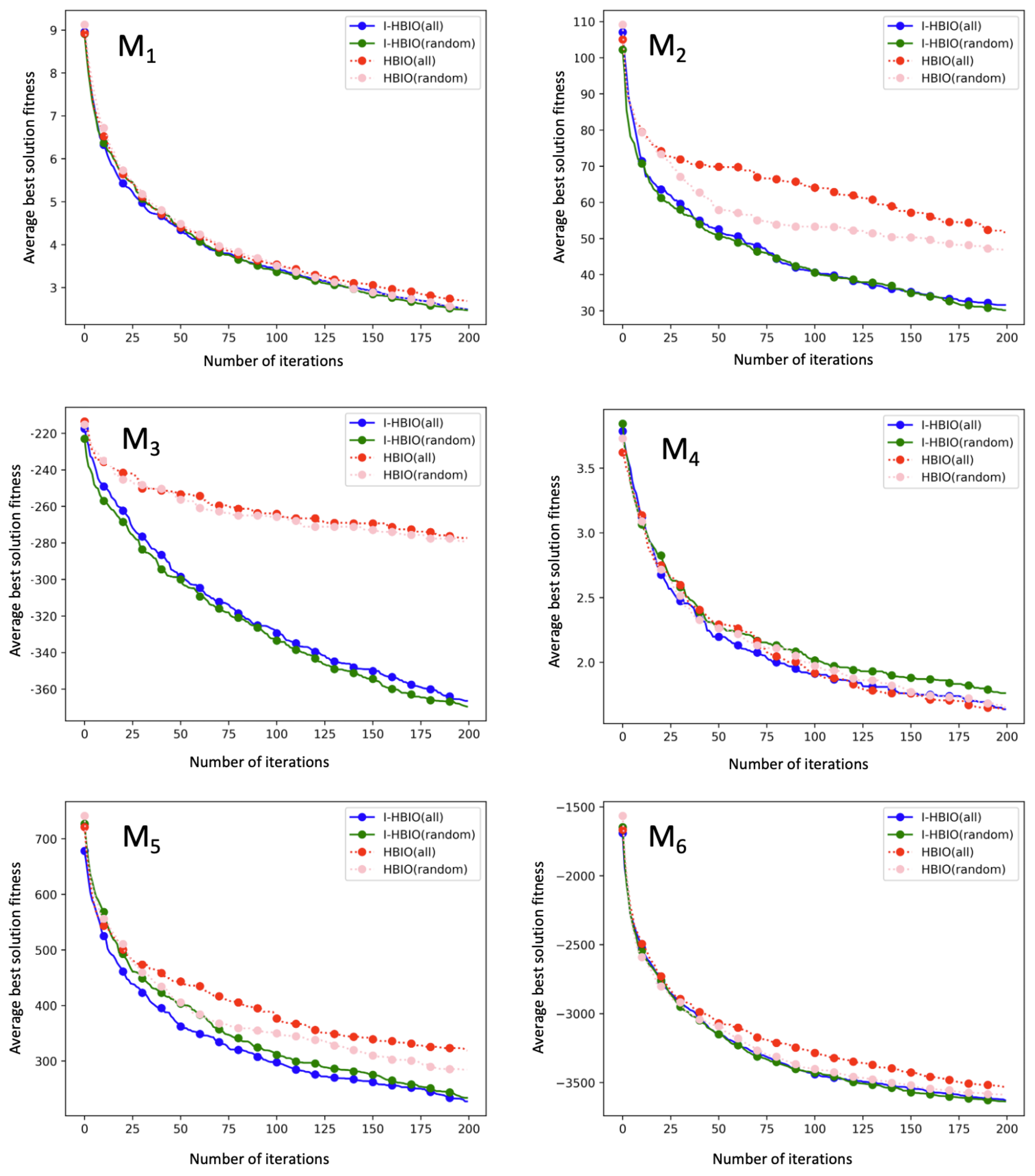
4.3. I-HBIA Algorithm Performances
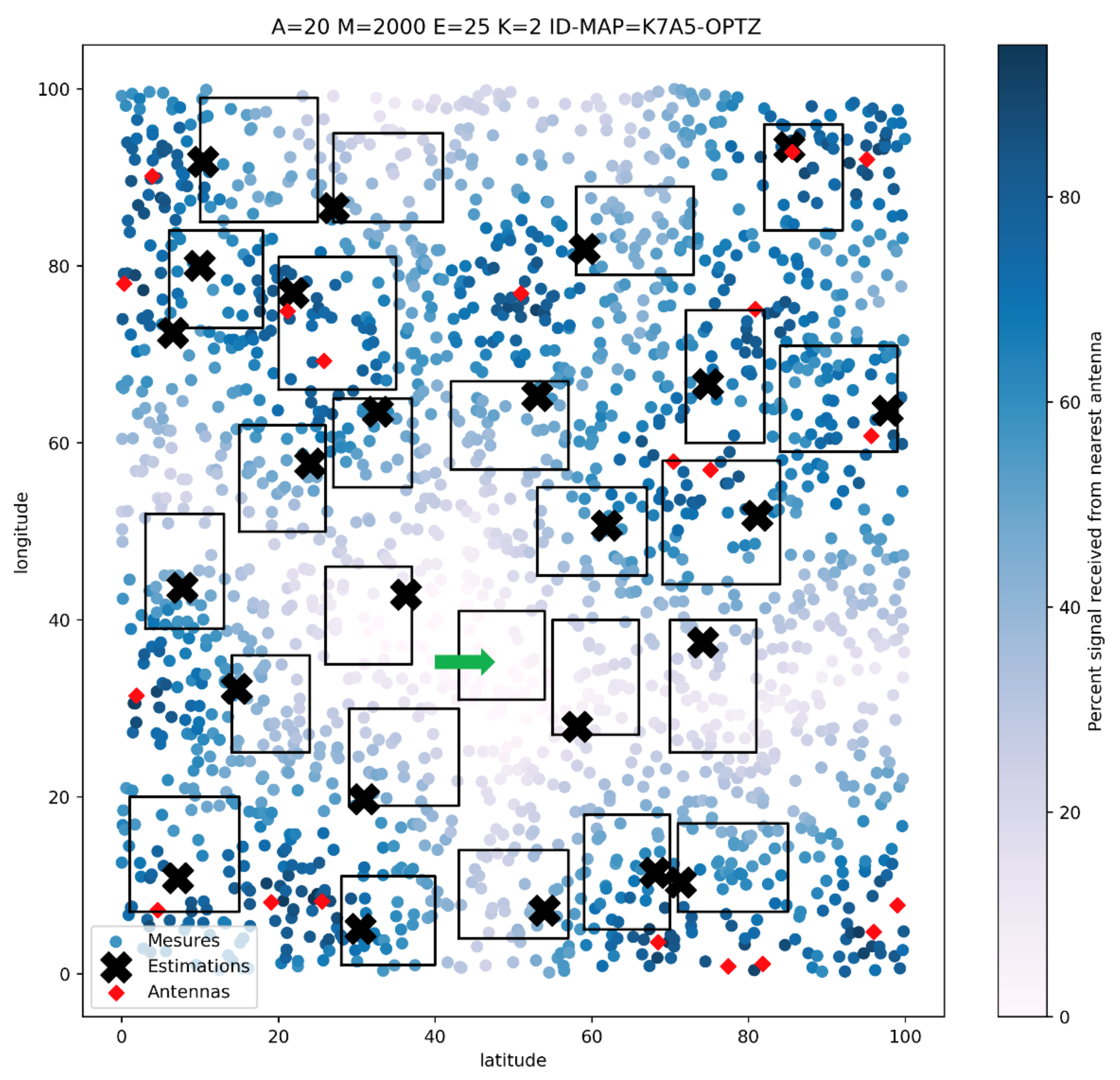
4.4. KNN and I-HBIA for WSN Deployment
5. Conclusions
Author Contributions
Funding
Institutional Review Board Statement
Informed Consent Statement
Data Availability Statement
Conflicts of Interest
References
- Idrees, Z.; Zheng, L. Low cost air pollution monitoring systems: A review of protocols and enabling technologies. J. Ind. Inf. Integr. 2020, 17, 100123. [Google Scholar] [CrossRef]
- Salman, N.; Kemp, A.H.; Khan, A.; Noakes, C. Real Time Wireless Sensor Network (WSN) based Indoor Air Quality Monitoring System. IFAC-PapersOnLine 2019, 52, 324–327. [Google Scholar] [CrossRef]
- Rehman, A.U.; Abbasi, A.Z.; Islam, N.; Shaikh, Z.A. A review of wireless sensors and networks’ applications in agriculture. Comput. Stand. Interfaces 2014, 36, 263–270. [Google Scholar] [CrossRef]
- Zhang, Y.; Sun, L.; Song, H.; Cao, X. Ubiquitous WSN for Healthcare: Recent Advances and Future Prospects. IEEE Internet Things J. 2014, 1, 311–318. [Google Scholar] [CrossRef]
- Moorthy, H.R.; Bangera, V.; Amrin, Z.; Avinash, N.; Rao, N.S.K. WSN in Defence Field: A Security Overview. In Proceedings of the 2020 Fourth International Conference on I-SMAC (IoT in Social, Mobile, Analytics and Cloud) (I-SMAC), Palladam, India, 7–9 October 2020; pp. 258–264. [Google Scholar] [CrossRef]
- Asorey-Cacheda, R.; Garcia-Sanchez, A.J.; Garcia-Sanchez, F.; Garcia-Haro, J. A survey on non-linear optimization problems in wireless sensor networks. J. Netw. Comput. Appl. 2017, 82, 1–20. [Google Scholar] [CrossRef]
- Farsi, M.; Elhosseini, M.A.; Badawy, M.; Arafat Ali, H.; Zain Eldin, H. Deployment Techniques in Wireless Sensor Networks, Coverage and Connectivity: A Survey. IEEE Access 2019, 7, 28940–28954. [Google Scholar] [CrossRef]
- Adnan, T.; Datta, S.; MacLean, S. Effcient and Accurate Range-based Sensor Network Localization. Procedia Comput. Sci. 2012, 10, 405–413. [Google Scholar] [CrossRef] [Green Version]
- Luomala, J.; Hakala, I. Adaptive range-based localization algorithm based on trilateration and reference node selection for outdoor wireless sensor networks. Comput. Netw. 2022, 210, 108865. [Google Scholar] [CrossRef]
- Pandey, S.; Varma, S. A Range Based Localization System in Multihop Wireless Sensor Networks: A Distributed Cooperative Approach. Wirel. Pers. Commun. 2016, 86, 615–634. [Google Scholar] [CrossRef]
- Khan, H.; Hayat, M.N.; Ur Rehman, Z. Wireless sensor networks free-range base localization schemes: A comprehensive survey. In Proceedings of the 2017 International Conference on Communication, Computing and Digital Systems (C-CODE), Islamabad, Pakistan, 8–9 March 2017; pp. 144–147. [Google Scholar] [CrossRef]
- Singh, S.P.; Sharma, S.C. Range Free Localization Techniques in Wireless Sensor Networks: A Review. Procedia Comput. Sci. 2015, 57, 7–16. [Google Scholar] [CrossRef] [Green Version]
- Jin, Y.; Zhou, L.; Zhang, L.; Hu, Z.; Han, J. A Novel Range-Free Node Localization Method for Wireless Sensor Networks. IEEE Wirel. Commun. Lett. 2022, 11, 688–692. [Google Scholar] [CrossRef]
- Cheikhrouhou, O.; Bhatti, G.M.; Alroobaea, R. A Hybrid DV-Hop Algorithm Using RSSI for Localization in Large-Scale Wireless Sensor Networks. Sensors 2018, 18, 1469. [Google Scholar] [CrossRef] [PubMed] [Green Version]
- Gui, L.; Xiao, F.; Zhou, Y.; Shu, F.; Val, T. Connectivity Based DV-Hop Localization for Internet of Things. IEEE Trans. Veh. Technol. 2020, 69, 8949–8958. [Google Scholar] [CrossRef]
- Dasgupta, S.; Mao, G.; Anderson, B. A New Measure of Wireless Network Connectivity. IEEE Trans. Mob. Comput. 2015, 14, 1765–1779. [Google Scholar] [CrossRef]
- Zhu, C.; Zheng, C.; Shu, L.; Han, G. A survey on coverage and connectivity issues in wireless sensor networks. J. Netw. Comput. Appl. 2012, 35, 619–632. [Google Scholar] [CrossRef]
- Liu, Y.; Suo, L.; Sun, D.; Wang, A. A Virtual Square Grid-Based Coverage Algorithm of Redundant Node for Wireless Sensor Network. J. Netw. Comput. Appl. 2013, 36, 811–817. [Google Scholar] [CrossRef]
- Fadi, M.A.T.; Hossam, S.H.; Mohamed, A.I. Quantifying connectivity of grid-based Wireless Sensor Networks under practical errors. In Proceedings of the IEEE Local Computer Network Conference, Denver, CO, USA, 10–14 October 2010; pp. 220–223. [Google Scholar] [CrossRef]
- Yu, X.; Liu, N.; Huang, W.; Qian, X.; Zhang, T. A Node Deployment Algorithm Based on Van Der Waals Force in Wireless Sensor Networks. Int. J. Distrib. Sens. Netw. 2013, 9, 505710. [Google Scholar] [CrossRef]
- Mahboubi, H.; Aghdam, A.G. Distributed Deployment Algorithms for Coverage Improvement in a Network of Wireless Mobile Sensors: Relocation by Virtual Force. IEEE Trans. Control Netw. Syst. 2017, 4, 736–748. [Google Scholar] [CrossRef]
- Wang, S.Y.; Shih, K.P.; Chen, Y.D.; Ku, H.H. Preserving Target Area Coverage in Wireless Sensor Networks by Using Computational Geometry. In Proceedings of the 2010 IEEE Wireless Communication and Networking Conference, Sydney, Australia, 18–21 April 2010; pp. 1–6. [Google Scholar] [CrossRef]
- Wu, C.H.; Lee, K.C.; Chung, Y.C. A Delaunay Triangulation based method for wireless sensor network deployment. Comput. Commun. 2007, 30, 2744–2752. [Google Scholar] [CrossRef]
- Wang, B. Coverage Problems in Sensor Networks: A Survey. ACM Comput. Surv. 2011, 43, 1–53. [Google Scholar] [CrossRef]
- Deif, D.S.; Gadallah, Y. Classification of Wireless Sensor Networks Deployment Techniques. IEEE Commun. Surv. Tutor. 2014, 16, 834–855. [Google Scholar] [CrossRef]
- Naik, C.; Shetty, D.P. A novel meta-heuristic differential evolution algorithm for optimal target coverage in wireless sensor networks. In International Conference on Innovations in Bio-Inspired Computing and Applications; Springer: Berlin/Heidelberg, Germany, 2018; pp. 83–92. [Google Scholar]
- Chand, S.; Kumar, B. Genetic algorithm-based meta-heuristic for target coverage problem. IET Wirel. Sens. Syst. 2018, 8, 170–175. [Google Scholar]
- Singh, S.; Kumar, S.; Nayyar, A.; Al-Turjman, F.; Mostarda, L. Proficient QoS-based target coverage problem in wireless sensor networks. IEEE Access 2020, 8, 74315–74325. [Google Scholar]
- Karatas, M. Optimal deployment of heterogeneous sensor networks for a hybrid point and barrier coverage application. Comput. Netw. 2018, 132, 129–144. [Google Scholar] [CrossRef]
- Mishra, P.; Kumar, N.; Godfrey, W.W. A Meta-heuristic-based Green-routing Algorithm in Software-Defined Wireless Sensor Network. In Proceedings of the 2021 6th International Conference on Inventive Computation Technologies (ICICT), Coimbatore, India, 20–22 January 2021; pp. 36–41. [Google Scholar] [CrossRef]
- El Ghazi, A.; Ahiod, B. Random waypoint impact on bio-inspired routing protocols in WSN. In Proceedings of the 2016 7th International Conference on Sciences of Electronics, Technologies of Information and Telecommunications (SETIT), Hammamet, Tunisia, 18–20 December 2016; pp. 326–331. [Google Scholar] [CrossRef]
- Gui, T.; Ma, C.; Wang, F.; Wilkins, D.E. Survey on swarm intelligence based routing protocols for wireless sensor networks: An extensive study. In Proceedings of the 2016 IEEE International Conference on Industrial Technology (ICIT), Taipei, Taiwan, 14–17 March 2016; pp. 1944–1949. [Google Scholar] [CrossRef]
- Zhao, X.; Ren, S.; Quan, H.; Gao, Q. Routing Protocol for Heterogeneous Wireless Sensor Networks Based on a Modified Grey Wolf Optimizer. Sensors 2020, 20, 820. [Google Scholar] [CrossRef]
- Ayedi, M.; Eldesouky, E.; Nazeer, J. Energy-Spectral Efficiency Optimization in Wireless Underground Sensor Networks Using Salp Swarm Algorithm. J. Sens. 2021, 2021, 6683988. [Google Scholar] [CrossRef]
- Esmaeili, H.; Bidgoli, B.M.; Hakami, V. CMML: Combined metaheuristic-machine learning for adaptable routing in clustered wireless sensor networks. Appl. Soft Comput. 2022, 118, 108477. [Google Scholar] [CrossRef]
- Tsai, C.W.; Hong, T.P.; Shiu, G.N. Metaheuristics for the Lifetime of WSN: A Review. IEEE Sens. J. 2016, 16, 2812–2831. [Google Scholar] [CrossRef]
- Gambhir, A.; Payal, A.; Arya, R. Chicken Swarm Optimization Algorithm Perspective on Energy Constraints in WSN. In Proceedings of the 2020 IEEE 7th Uttar Pradesh Section International Conference on Electrical, Electronics and Computer Engineering (UPCON), Prayagraj, India, 27–29 November 2020; pp. 1–5. [Google Scholar] [CrossRef]
- Wang, H.; Li, K.; Pedrycz, W. An Elite Hybrid Metaheuristic Optimization Algorithm for Maximizing Wireless Sensor Networks Lifetime with a Sink Node. IEEE Sens. J. 2020, 20, 5634–5649. [Google Scholar] [CrossRef]
- Abba Ari, A.A.; Gueroui, A.; Yenke, B.O.; Labraoui, N. Energy efficient clustering algorithm for Wireless Sensor Networks using the ABC metaheuristic. In Proceedings of the 2016 International Conference on Computer Communication and Informatics (ICCCI), Coimbatore, India, 7–9 January 2016; pp. 1–6. [Google Scholar] [CrossRef]
- Chung, V.; Tuah, N.; Lim, K.G.; Tan, M.K.; Saad, I.; Kin Teo, K.T. Metaheuristic Multi-Hop Clustering Optimization for Energy-Efficient Wireless Sensor Network. In Proceedings of the 2020 IEEE 2nd International Conference on Artificial Intelligence in Engineering and Technology (IICAIET), Kota Kinabalu, Malaysia, 26–27 September 2020; pp. 1–6. [Google Scholar] [CrossRef]
- Zivkovic, M.; Bacanin, N.; Zivkovic, T.; Strumberger, I.; Tuba, E.; Tuba, M. Enhanced Grey Wolf Algorithm for Energy Efficient Wireless Sensor Networks. In Proceedings of the 2020 Zooming Innovation in Consumer Technologies Conference (ZINC), Novi Sad, Serbia, 26–27 May 2020; pp. 87–92. [Google Scholar] [CrossRef]
- Mohamed, A.; Saber, W.; Elnahry, I.; Hassanien, A.E. Coyote Optimization Based on a Fuzzy Logic Algorithm for Energy-Efficiency in Wireless Sensor Networks. IEEE Access 2020, 8, 185816–185829. [Google Scholar] [CrossRef]
- Tuba, E.; Simian, D.; Dolicanin, E.; Jovanovic, R.; Tuba, M. Energy Efficient Sink Placement in Wireless Sensor Networks by Brain Storm Optimization Algorithm. In Proceedings of the 2018 14th International Wireless Communications Mobile Computing Conference (IWCMC), Limassol, Cyprus, 25–29 June 2018; pp. 718–723. [Google Scholar] [CrossRef]
- Shankar, T.; Eappen, G.; Sahani, S.; Rajesh, A.; Mageshvaran, R. Integrated Cuckoo and Monkey Search Algorithm for Energy Efficient Clustering in Wireless Sensor Networks. In Proceedings of the 2019 Innovations in Power and Advanced Computing Technologies (i-PACT), Vellore, India, 22–23 March 2019; Volume 1, pp. 1–4. [Google Scholar] [CrossRef]
- Zivkovic, M.; Bacanin, N.; Tuba, E.; Strumberger, I.; Bezdan, T.; Tuba, M. Wireless Sensor Networks Life Time Optimization Based on the Improved Firefly Algorithm. In Proceedings of the 2020 International Wireless Communications and Mobile Computing (IWCMC), Limassol, Cyprus, 15–19 June 2020; pp. 1176–1181. [Google Scholar] [CrossRef]
- Tsai, C.W.; Tsai, P.W.; Pan, J.S.; Chao, H.C. Metaheuristics for the deployment problem of WSN: A review. Microprocess. Microsyst. 2015, 39, 1305–1317. [Google Scholar] [CrossRef]
- Liao, W.H.; Kao, Y.; Li, Y.S. A sensor deployment approach using glowworm swarm optimization algorithm in wireless sensor networks. Expert Syst. Appl. 2011, 38, 12180–12188. [Google Scholar] [CrossRef]
- Metiaf, A.; Wu, Q. Particle Swarm Optimization Based Deployment for WSN with the Existence of Obstacles. In Proceedings of the 2019 5th International Conference on Control, Automation and Robotics (ICCAR), Beijing, China, 19–22 April 2019. [Google Scholar]
- Kumar, G.; Ranga, V. Meta-heuristics for relay node placement problem in wireless sensor networks. In Proceedings of the 2016 Fourth International Conference on Parallel, Distributed and Grid Computing (PDGC), Waknaghat, India, 22–24 December 2016; pp. 375–380. [Google Scholar] [CrossRef]
- Ng, C.K.; Wu, C.H.; Ip, W.H.; Yung, K.L. A Smart Bat Algorithm for Wireless Sensor Network Deployment in 3-D Environment. IEEE Commun. Lett. 2018, 22, 2120–2123. [Google Scholar] [CrossRef]
- Arsic, A.; Tuba, M.; Jordanski, M. Fireworks algorithm applied to wireless sensor networks localization problem. In Proceedings of the 2016 IEEE Congress on Evolutionary Computation (CEC), Vancouver, BC, Canada, 24–29 July 2016; pp. 4038–4044. [Google Scholar] [CrossRef]
- Das, P.P.; Chakraborty, N.; Allayear, S.M. Optimal coverage of Wireless Sensor Network using Termite Colony Optimization Algorithm. In Proceedings of the 2015 International Conference on Electrical Engineering and Information Communication Technology (ICEEICT), Dhaka, Bangladesh, 21–23 May 2015; pp. 1–6. [Google Scholar] [CrossRef]
- Ghosh, S.; Snigdh, I.; Singh, A. GA optimal sink placement for maximizing coverage in Wireless Sensor Networks. In Proceedings of the 2016 International Conference on Wireless Communications, Signal Processing and Networking (WiSPNET), Chennai, India, 23–25 March 2016; pp. 737–741. [Google Scholar] [CrossRef]
- Aziz, N.A.A.; Aziz, N.H.A.; Aziz, K.A.; Ibrahim, Z.; Aliman, M.N. Evaluation of Pure Gravitational Search Algorithm for Wireless Sensor Networks Coverage Maximization. In Proceedings of the 2018 International Electrical Engineering Congress (iEECON), Krabi, Thailand, 7–9 March 2018; pp. 1–4. [Google Scholar] [CrossRef]
- Strumberger, I.; Tuba, E.; Bacanin, N.; Beko, M.; Tuba, M. Wireless Sensor Network Localization Problem by Hybridized Moth Search Algorithm. In Proceedings of the 2018 14th International Wireless Communications Mobile Computing Conference (IWCMC), Limassol, Cyprus, 25–29 June 2018; pp. 316–321. [Google Scholar] [CrossRef]
- Sabbella, V.R.; Edla, D.R.; Lipare, A.; Parne, S.R. An Efficient Localization Approach in Wireless Sensor Networks Using Krill Herd Optimization Algorithm. IEEE Syst. J. 2021, 15, 2432–2442. [Google Scholar] [CrossRef]
- Strumberger, I.; Tuba, E.; Bacanin, N.; Beko, M.; Tuba, M. Monarch butterfly optimization algorithm for localization in wireless sensor networks. In Proceedings of the 2018 28th International Conference Radioelektronika (RADIOELEKTRONIKA), Prague, Czech Republic, 19–20 April 2018; pp. 1–6. [Google Scholar] [CrossRef]
- Shindarov, M.; Fidanova, S.; Marinov, P. Wireless sensor positioning algorithm. In Proceedings of the 2012 6th IEEE International Conference Intelligent Systems, Sofia, Bulgaria, 6–8 September 2012; pp. 419–424. [Google Scholar] [CrossRef]
- Deif, D.; Gadallah, Y. Wireless Sensor Network deployment using stochastic optimization techniques—A comparative study. In Proceedings of the 2015 International Conference on Computing and Network Communications (CoCoNet), Trivandrum, India, 16–19 December 2015; pp. 131–138. [Google Scholar] [CrossRef]
- Alia, O.M.; Al-Ajouri, A. Maximizing Wireless Sensor Network Coverage with Minimum Cost Using Harmony Search Algorithm. IEEE Sens. J. 2017, 17, 882–896. [Google Scholar] [CrossRef]
- Idrees, Z.; Zheng, L. No free lunch theorems for optimization. IEEE Trans. Evol. Comput. 1997, 17, 67–82. [Google Scholar]
- Storn, R.; Price, K. Differential Evolution—A Simple and Efficient Heuristic for global Optimization over Continuous Spaces. J. Glob. Optim. 1997, 11, 341–359. [Google Scholar] [CrossRef]
- Holland, J.H.; Reitman, J.S. Cognitive systems based on adaptive algorithms. SIGART Newsl. 1977, 63, 49. [Google Scholar] [CrossRef]
- Dorigo, M.; Birattari, M.; Stutzle, T. Ant colony optimization. IEEE Comput. Intell. Mag. 2006, 1, 28–39. [Google Scholar] [CrossRef]
- Kennedy, J.; Eberhart, R. Particle swarm optimization. In Proceedings of the ICNN’95—International Conference on Neural Networks, Perth, WA, Australia, 27 November–1 December 1995; Volume 4, pp. 1942–1948. [Google Scholar] [CrossRef]
- Mirjalili, S.; Mirjalili, S.M.; Lewis, A. Grey Wolf Optimizer. Adv. Eng. Softw. 2014, 69, 46–61. [Google Scholar] [CrossRef] [Green Version]
- Mirjalili, S.; Lewis, A. The Whale Optimization Algorithm. Adv. Eng. Softw. 2016, 95, 51–67. [Google Scholar] [CrossRef]
- Mirjalili, S. Moth-flame optimization algorithm: A novel nature-inspired heuristic paradigm. Knowl.-Based Syst. 2015, 89, 228–249. [Google Scholar] [CrossRef]
- Abedinpourshotorban, H.; Mariyam Shamsuddin, S.; Beheshti, Z.; Jawawi, D.N.A. Electromagnetic field optimization: A physics-inspired metaheuristic optimization algorithm. Swarm Evol. Comput. 2016, 26, 8–22. [Google Scholar] [CrossRef]
- Azizi, M. Atomic orbital search: A novel metaheuristic algorithm. Appl. Math. Model. 2021, 93, 657–683. [Google Scholar] [CrossRef]
- Rashedi, E.; Nezamabadi-pour, H.; Saryazdi, S. GSA: A Gravitational Search Algorithm. Inf. Sci. 2009, 179, 2232–2248. [Google Scholar] [CrossRef]
- Ghasemian, H.; Ghasemian, F.; Vahdat-Nejad, H. Human urbanization algorithm: A novel metaheuristic approach. Math. Comput. Simul. 2020, 178, 1–15. [Google Scholar] [CrossRef]
- Mousavirad, S.J.; Ebrahimpour-Komleh, H. Human mental search: A new population-based metaheuristic optimization algorithm. Appl. Intell. 2017, 47, 850–887. [Google Scholar] [CrossRef]
- Salih, S.Q.; Alsewari, A.A. A new algorithm for normal and large-scale optimization problems: Nomadic People Optimizer. Neural Comput. Appl. 2020, 32, 10359–10386. [Google Scholar] [CrossRef]
- Kirkpatrick, S.; Gelatt, C.D.; Vecchi, M.P. Optimization by Simulated Annealing. Science 1983, 220, 671–680. [Google Scholar] [CrossRef]
- Mirjalili, S. The Ant Lion Optimizer. Adv. Eng. Softw. 2015, 83, 80–98. [Google Scholar] [CrossRef]
- Mirjalili, S. SCA: A Sine Cosine Algorithm for solving optimization problems. Knowl.-Based Syst. 2016, 96, 120–133. [Google Scholar] [CrossRef]
- Sarker, I.H. Machine Learning: Algorithms, Real-World Applications and Research Directions. SN Comput. Sci. 2021, 2, 160. [Google Scholar] [CrossRef] [PubMed]
- Ray, S. A quick review of machine learning algorithms. In Proceedings of the 2019 International Conference on Machine Learning, Big Data, Cloud and Parallel Computing (COMITCon), Faridabad, India, 14–16 February 2019; IEEE: Piscataway, NJ, USA, 2019; pp. 35–39. [Google Scholar]
- Arrieta, A.B.; Díaz-Rodríguez, N.; Ser, J.D.; Bennetot, A.; Tabik, S.; Barbado, A.; Garcia, S.; Gil-Lopez, S.; Molina, D.; Benjamins, R.; et al. Explainable Artificial Intelligence (XAI): Concepts, taxonomies, opportunities and challenges toward responsible AI. Inf. Fusion 2020, 58, 82–115. [Google Scholar] [CrossRef] [Green Version]
- Yang, L.; Shami, A. On Hyperparameter Optimization of Machine Learning Algorithms: Theory and Practice. arXiv 2020, arXiv:2007.15745. [Google Scholar] [CrossRef]
- Fix, E.; Hodges, J.L. Discriminatory Analysis—Nonparametric Discrimination: Consistency Properties. Int. Stat. Rev. 1989, 57, 238. [Google Scholar] [CrossRef]
- Zhang, S.; Cheng, D.; Deng, Z.; Zong, M.; Deng, X. A novel kNN algorithm with data-driven k parameter computation. Pattern Recognit. Lett. 2018, 109, 44–54. [Google Scholar] [CrossRef]
- Morais, R.G.; Nedjah, N.; Mourelle, L.M. A novel metaheuristic inspired by Hitchcock birds’ behavior for efficient optimization of large search spaces of high dimensionality. Soft Comput. 2020, 24, 5633–5655. [Google Scholar] [CrossRef]


| Name | Publication Date | Inspiration |
|---|---|---|
| Simulated annealing [75] | 1983 | Physics |
| Differential evolution [62] | 1997 | Evolutionary |
| Particle swarm optimization [65] | 1995 | Swarm |
| Genetic algorithms [63] | 1962 | Evolutionary |
| Ant colony optimization [64] | 2006 | Swarm |
| Name | Publication Date | Inspiration |
|---|---|---|
| Grey wolves optimizer [66] | 2014 | Swarm |
| Whale optimization algorithm [67] | 2016 | Swarm |
| Ant lion optimization [76] | 2015 | Swarm |
| Moth-flame optimization [68] | 2015 | Swarm |
| Sine cosine algorithm [77] | 2016 | Mathematics |
| Parameters | Values |
|---|---|
| Number of measures | [200, 250, 500, 600, 700, 800, 900, 1000] |
| K values | [1–20] |
| Number of repetitions | 20 |
| Considering learning dataset | 80% |
| Considering testing dataset | 20% |
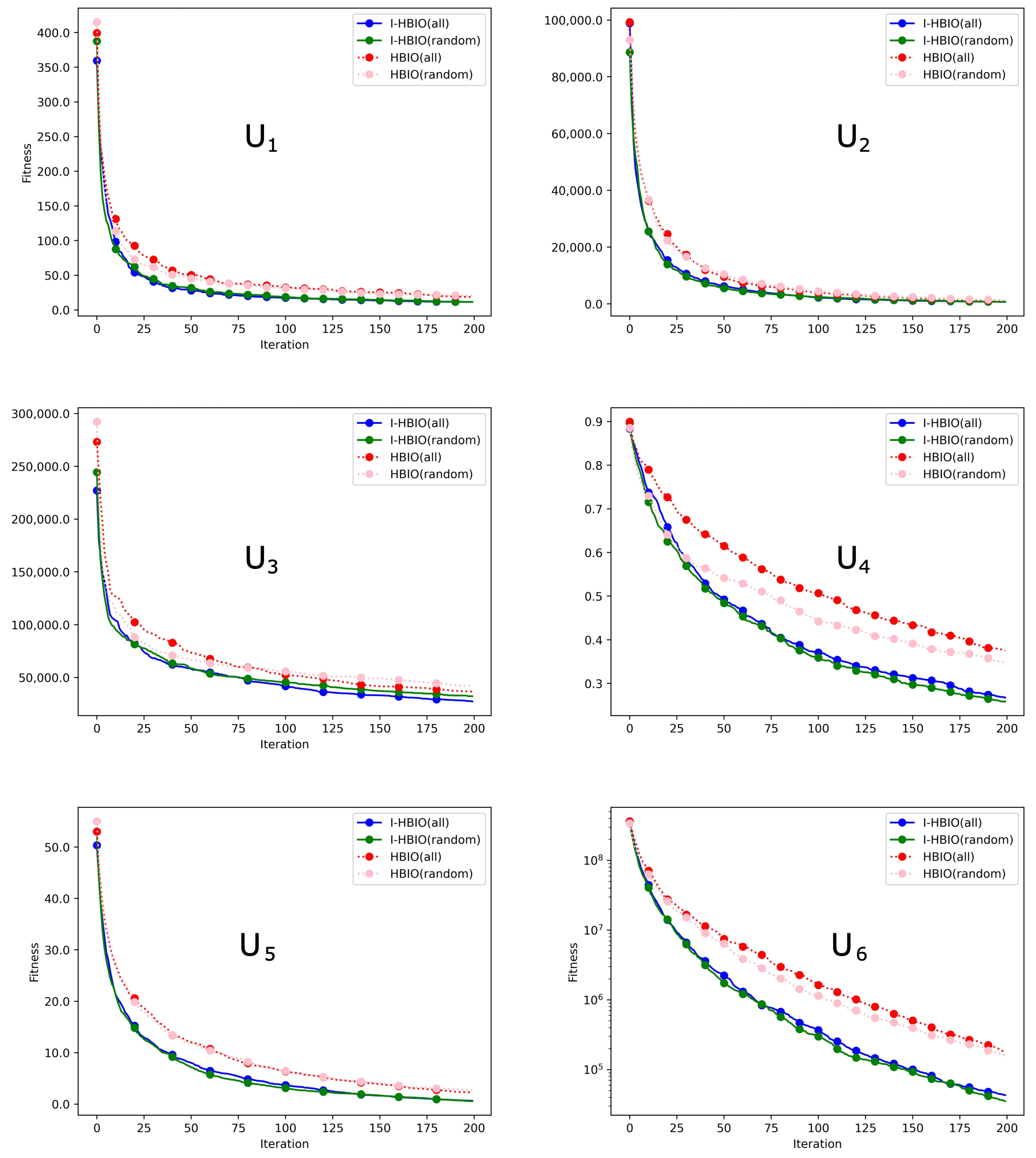
| Configuration | Local Search by Cloning | Dimension Consideration | Number of Iterations |
|---|---|---|---|
| HBIA (all) | Disabled | All dimensions | 200 |
| HBIA (random) | Disabled | Random dimensions | 200 |
| I-HBIA (all) | Enabled | All dimensions | 200 |
| I-HBIA (random) | Enabled | Random dimensions | 200 |
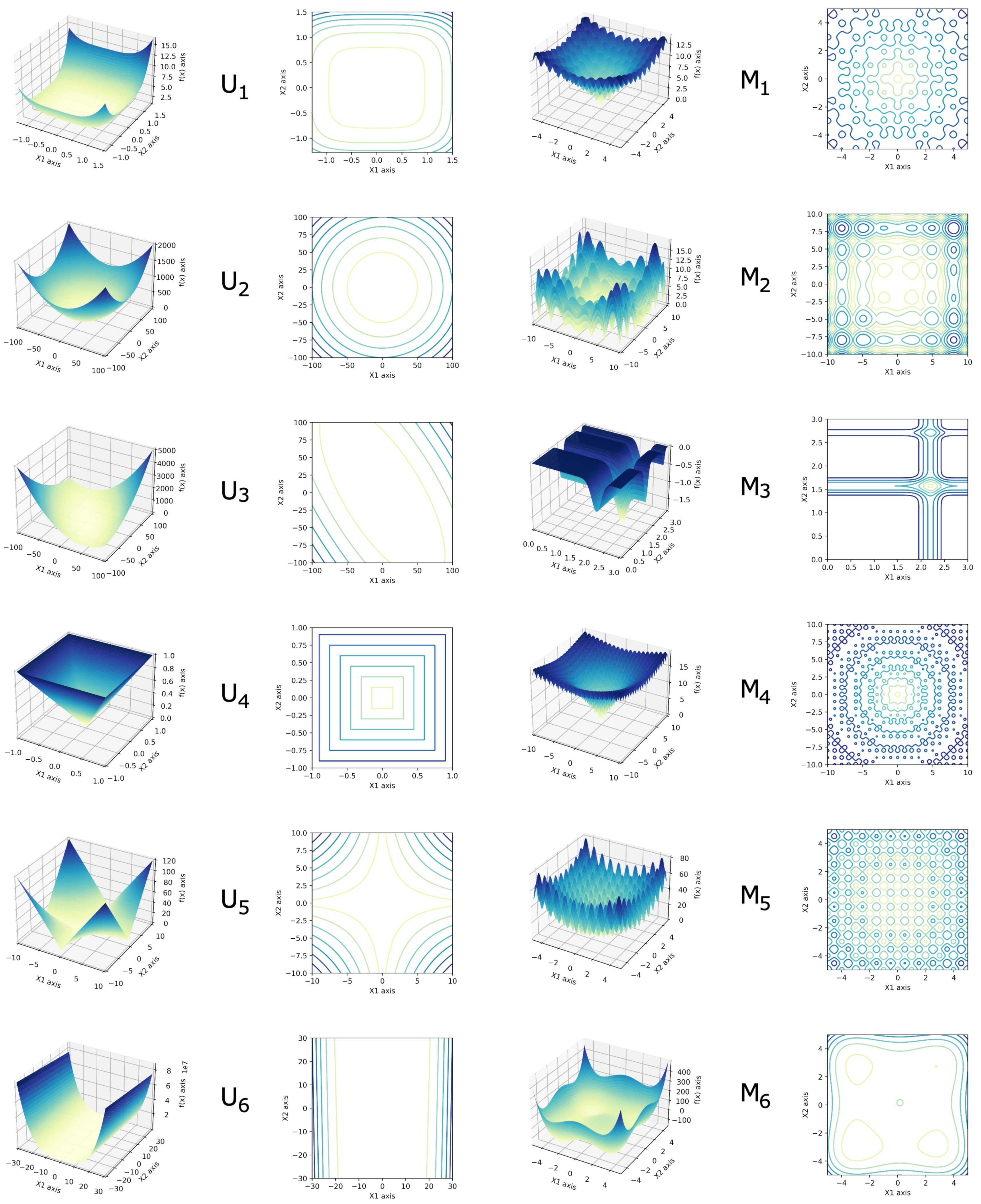
| Equation | Name | Dimension | Number of Iterations | Benchmark ID |
|---|---|---|---|---|
| Quartic | 50 | 200 | ||
| Sphere | 50 | 200 | ||
| Schwefel 1.22 | 50 | 200 | ||
| Schwefel 2.21 | 50 | 200 | ||
| Schwefel 2.22 | 50 | 200 | ||
| Rosenbrock | 50 | 200 |
| Equation | Nane | Dimension | Iterations | Benchmark ID |
|---|---|---|---|---|
| Ackley | 50 | 200 | ||
| Alpine | 50 | 200 | ||
| Michalewicz | 50 | 200 | ||
| Salomon | 50 | 200 | ||
| Rastringin | 50 | 200 | ||
| Styblinski Tank | 50 | 200 |
Publisher’s Note: MDPI stays neutral with regard to jurisdictional claims in published maps and institutional affiliations. |
© 2022 by the authors. Licensee MDPI, Basel, Switzerland. This article is an open access article distributed under the terms and conditions of the Creative Commons Attribution (CC BY) license (https://creativecommons.org/licenses/by/4.0/).
Share and Cite
Poggi, B.; Babatounde, C.; Vittori, E.; Antoine-Santoni, T. Efficient WSN Node Placement by Coupling KNN Machine Learning for Signal Estimations and I-HBIA Metaheuristic Algorithm for Node Position Optimization. Sensors 2022, 22, 9927. https://doi.org/10.3390/s22249927
Poggi B, Babatounde C, Vittori E, Antoine-Santoni T. Efficient WSN Node Placement by Coupling KNN Machine Learning for Signal Estimations and I-HBIA Metaheuristic Algorithm for Node Position Optimization. Sensors. 2022; 22(24):9927. https://doi.org/10.3390/s22249927
Chicago/Turabian StylePoggi, Bastien, Chabi Babatounde, Evelyne Vittori, and Thierry Antoine-Santoni. 2022. "Efficient WSN Node Placement by Coupling KNN Machine Learning for Signal Estimations and I-HBIA Metaheuristic Algorithm for Node Position Optimization" Sensors 22, no. 24: 9927. https://doi.org/10.3390/s22249927