
Explainable Artificial Intelligence Model for Stroke Prediction Using EEG Signal

 , and
, and
Abstract
:1. Introduction
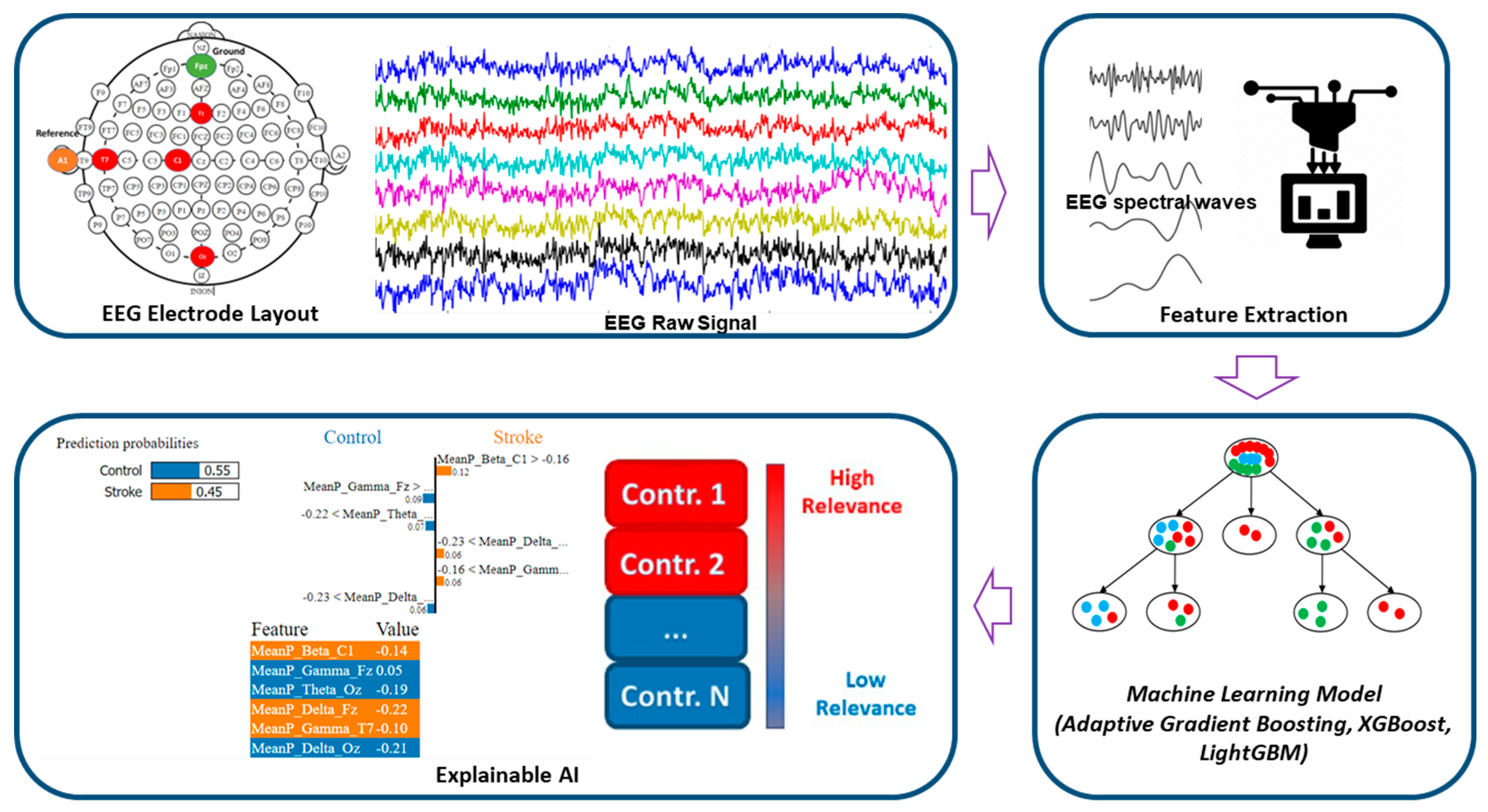
- We developed the ML models to classify the ischemic stroke group and the healthy control group for acute stroke prediction in an active state.
- We have used Eli5 to explain the behavior of the model as a whole to determine the significant features, which contribute to stroke prediction models.
- Further, we have utilized the LIME (Local Interpretable Model-Agnostic Explanations) method to interpret the prediction done by the model locally through a plethora of contributions from distinct EEG features.
2. Materials and Methods
2.1. EEG Data Description
2.2. EEG Signal Pre-Processing
2.3. Feature Extraction
2.4. Features Scaling
2.5. Machine-Learning Classification Algorithms
2.5.1. Adaptive Gradient Boosting (AdaBoost)
2.5.2. XGBoost
2.5.3. LightGBM
2.6. Machine-Learning Analysis and Performance Matrix
2.7. Explainable Artificial Intelligence (XAI)
2.7.1. Eli5
2.7.2. LIME
3. Results
3.1. Stroke Prediction Model Using Machine Learning Approach
3.1.1. Hyperparameter Tuning
3.1.2. ML Classification Results
3.2. Explanations of ML Models
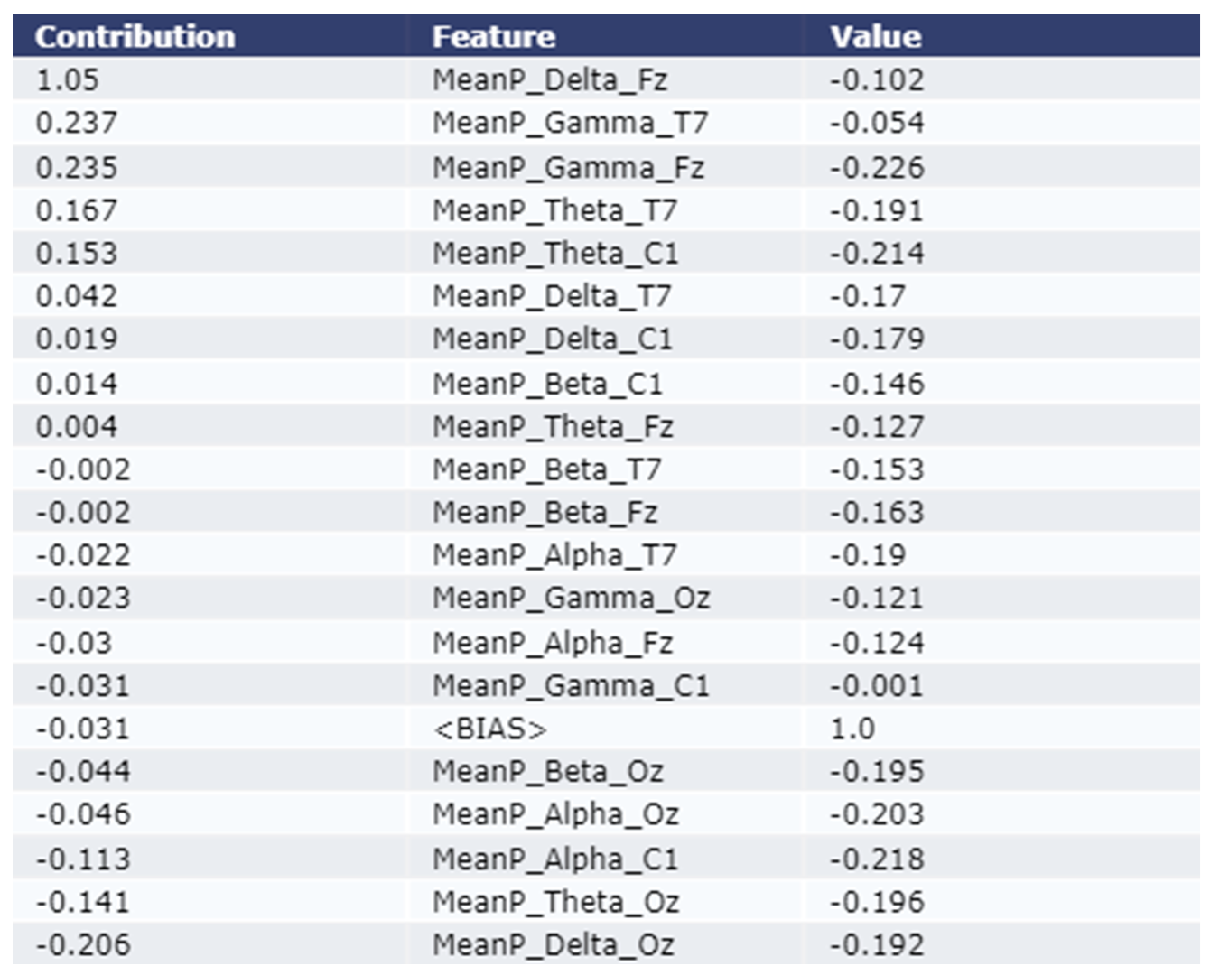
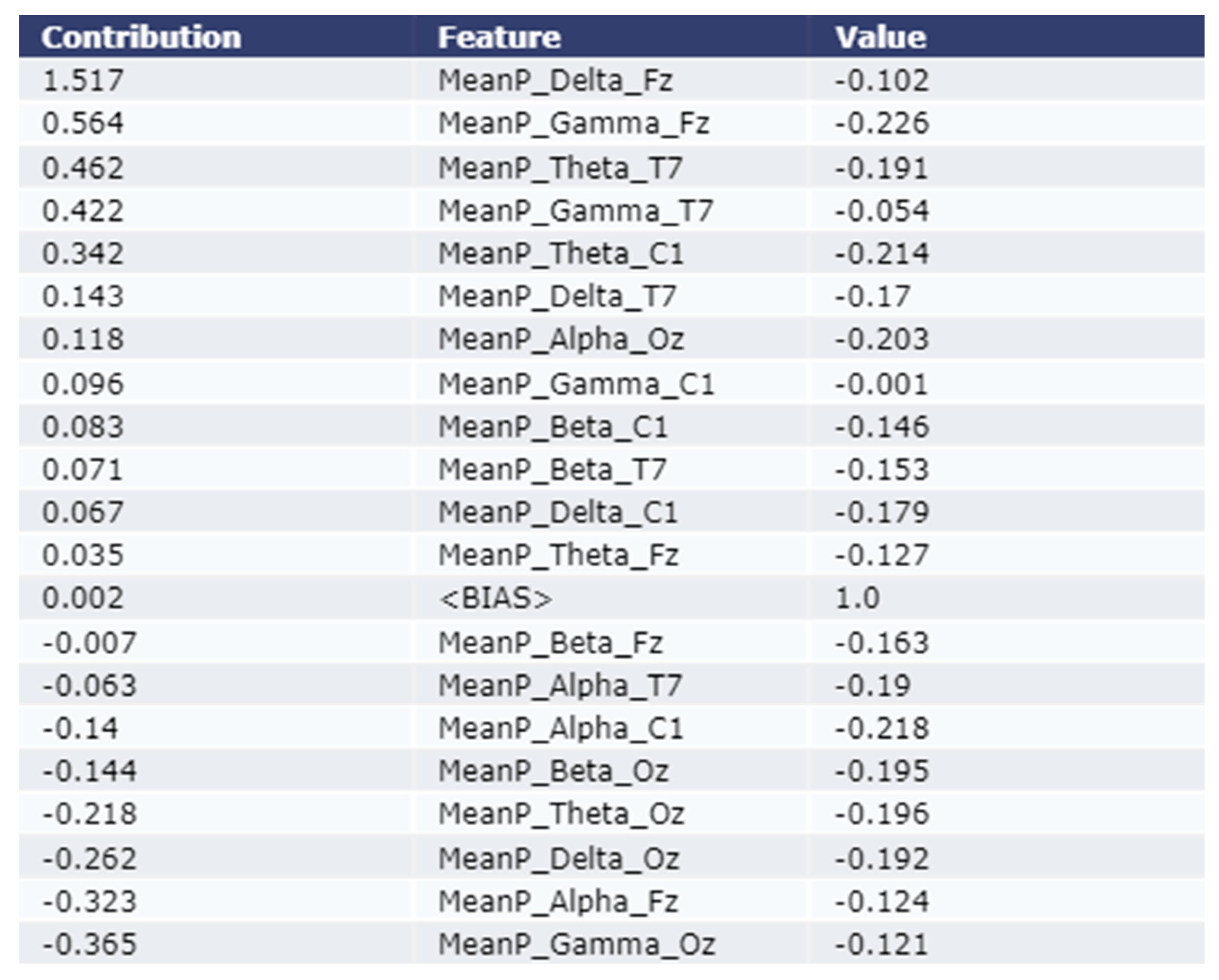
3.2.1. Model Explanation using Eli5
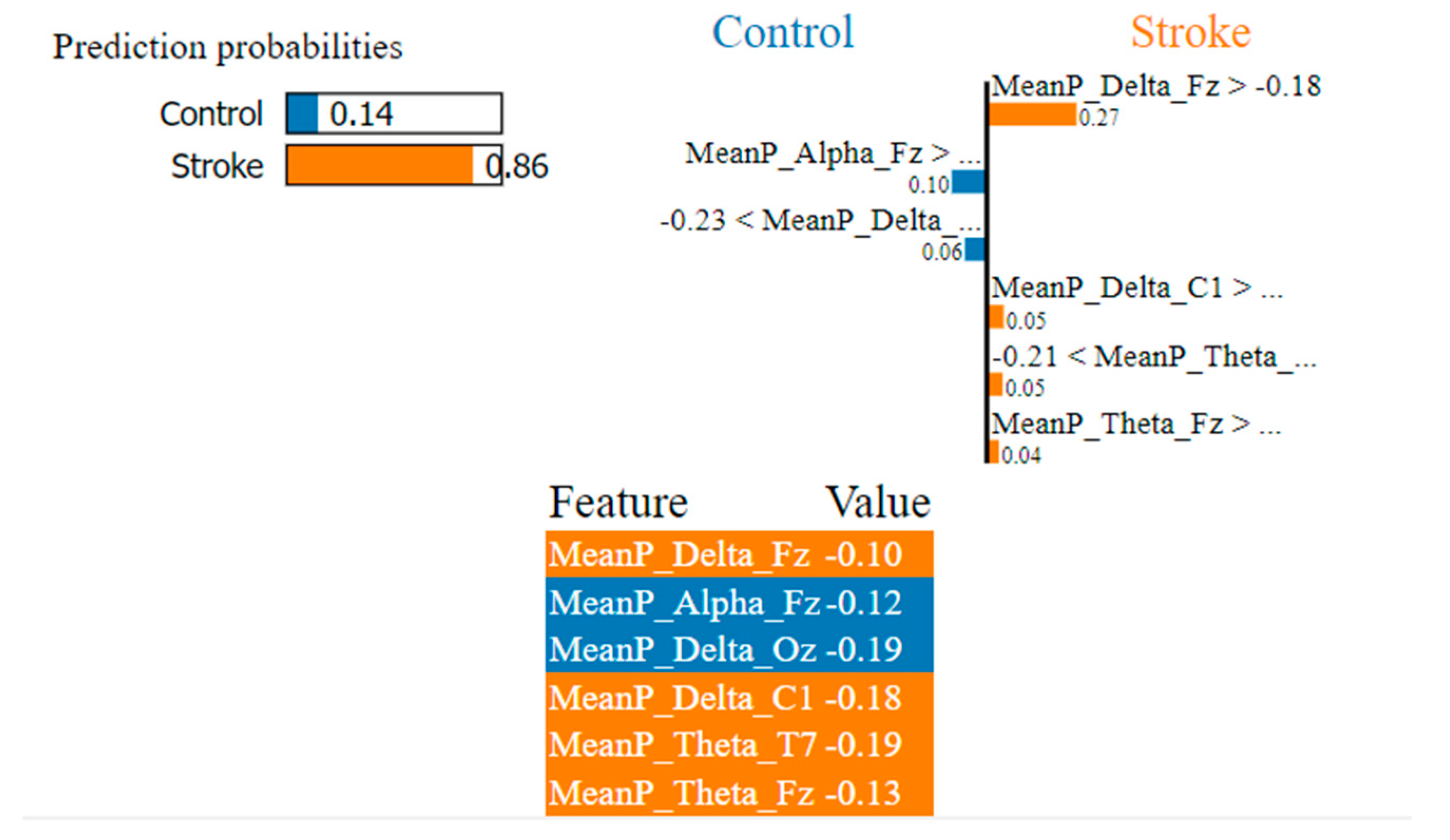
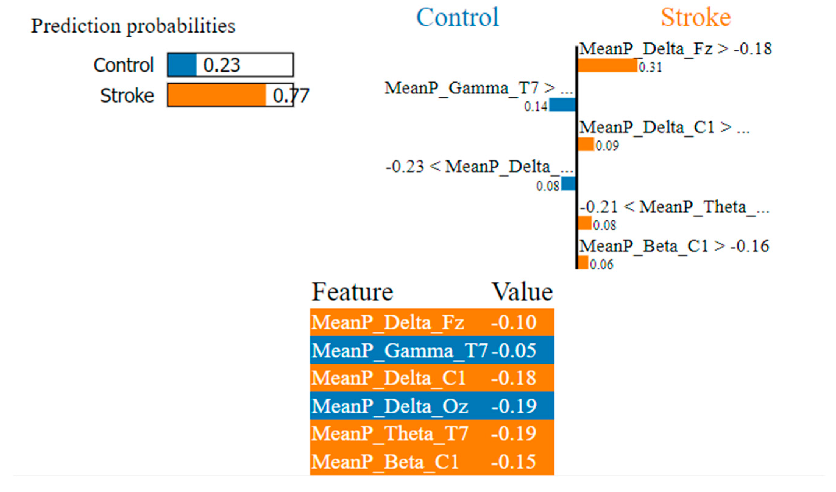
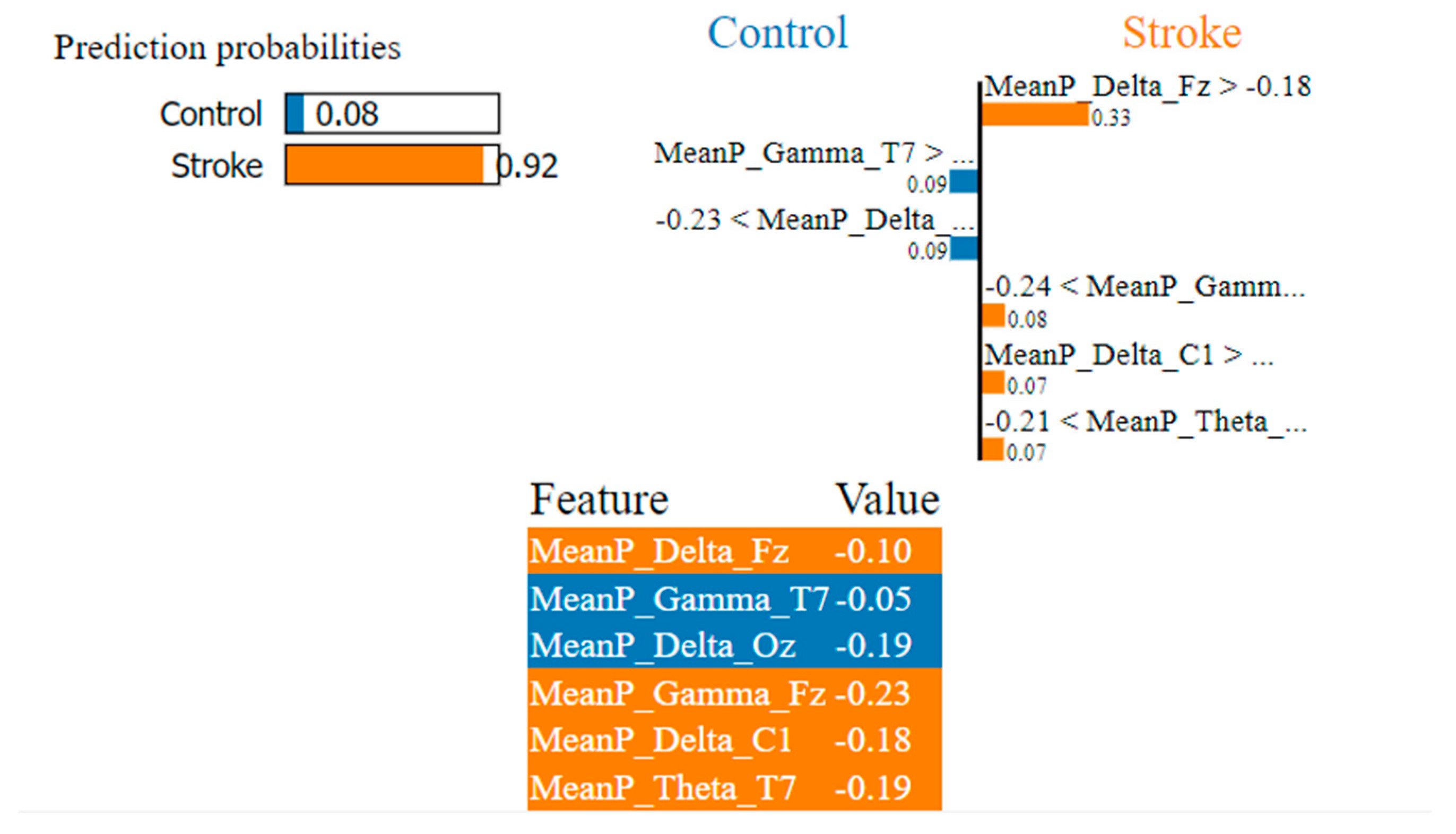
3.2.2. Model Explanation using LIME
4. Discussion
5. Conclusions
Author Contributions
Funding
Institutional Review Board Statement
Informed Consent Statement
Data Availability Statement
Acknowledgments
Conflicts of Interest
References
- Balami, J.S.; Chen, R.-L.; Grunwald, I.Q.; Buchan, A.M. Neurological complications of acute ischaemic stroke. Lancet Neurol. 2011, 10, 357–371. [Google Scholar] [CrossRef] [PubMed]
- Campbell, B.C.; De Silva, D.A.; Macleod, M.R.; Coutts, S.B.; Schwamm, L.H.; Davis, S.M.; Donnan, G.A. Ischaemic stroke. Nat. Rev. Dis. Prim. 2019, 5, 1–22. [Google Scholar] [CrossRef] [PubMed]
- Park, S.J.; Hong, S.; Kim, D.; Seo, Y.; Hussain, I.; Hur, J.H.; Jin, W. Development of a Real-Time Stroke Detection System for Elderly Drivers Using Quad-Chamber Air Cushion and IoT Devices. SAE Int. 2018. [Google Scholar] [CrossRef]
- Park, S.; Hong, S.; Kim, D.; Yu, J.; Hussain, I.; Park, H.; Benjamin, H. Development of Intelligent Stroke Monitoring System for the Elderly during Sleeping. Sleep Med. 2019, 64, S294. [Google Scholar] [CrossRef]
- Hussain, I.; Park, S.-J. Quantitative Evaluation of Task-Induced Neurological Outcome after Stroke. Brain Sci. 2021, 11, 900. [Google Scholar] [CrossRef]
- Aminov, A.; Rogers, J.M.; Johnstone, S.J.; Middleton, S.; Wilson, P.H. Acute single channel EEG predictors of cognitive function after stroke. PLoS ONE 2017, 12, e0185841. [Google Scholar] [CrossRef] [Green Version]
- Hussain, I.; Young, S.; Kim, C.H.; Benjamin, H.C.M.; Park, S.J. Quantifying Physiological Biomarkers of a Microwave Brain Stimulation Device. Sensors 2021, 21, 1896. [Google Scholar] [CrossRef]
- Park, S.J.; Hong, S.; Kim, D.; Hussain, I.; Seo, Y. Intelligent In-Car Health Monitoring System for Elderly Drivers in Connected Car. In Proceedings of the 20th Congress of the International Ergonomics Association (IEA 2018), Florence, Italy, 26–30 August 2018; pp. 40–44. [Google Scholar]
- Park, S.J.; Hong, S.; Kim, D.; Seo, Y.; Hussain, I. Knowledge Based Health Monitoring during Driving; Springer International Publishing: Cham, Switzerland, 2018; pp. 387–392. [Google Scholar]
- Hong, S.; Kim, D.; Park, H.; Seo, Y.; Iqram, H.; Park, S. Gait Feature Vectors for Post-stroke Prediction using Wearable Sensor. Korean Soc. Emot. Sensib. 2019, 22, 55–64. [Google Scholar] [CrossRef]
- Park, H.; Hong, S.; Hussain, I.; Kim, D.; Seo, Y.; Park, S.J. Gait Monitoring System for Stroke Prediction of Aging Adults. In Proceedings of the International Conference on Applied Human Factors and Ergonomics, Washington, DC, USA, 24–28 July 2019; pp. 93–97. [Google Scholar]
- van Putten, M.J.A.M.; Tavy, D.L.J. Continuous Quantitative EEG Monitoring in Hemispheric Stroke Patients Using the Brain Symmetry Index. Stroke 2004, 35, 2489–2492. [Google Scholar] [CrossRef] [Green Version]
- Xin, X.; Chang, J.; Gao, Y.; Shi, Y. Correlation Between the Revised Brain Symmetry Index, an EEG Feature Index, and Short-term Prognosis in Acute Ischemic Stroke. J. Clin. Neurophysiol. 2017, 34, 162–167. [Google Scholar] [CrossRef]
- Finnigan, S.P.; Rose, S.E.; Walsh, M.; Griffin, M.; Janke, A.L.; McMahon, K.L.; Gillies, R.; Strudwick, M.W.; Pettigrew, C.M.; Semple, J.; et al. Correlation of Quantitative EEG in Acute Ischemic Stroke with 30-Day NIHSS Score. Stroke 2004, 35, 899–903. [Google Scholar] [CrossRef] [PubMed]
- Finnigan, S.; Wong, A.; Read, S. Defining abnormal slow EEG activity in acute ischaemic stroke: Delta/alpha ratio as an optimal QEEG index. Clin. Neurophysiol. 2016, 127, 1452–1459. [Google Scholar] [CrossRef] [PubMed] [Green Version]
- Fanciullacci, C.; Bertolucci, F.; Lamola, G.; Panarese, A.; Artoni, F.; Micera, S.; Rossi, B.; Chisari, C. Delta Power Is Higher and More Symmetrical in Ischemic Stroke Patients with Cortical Involvement. Front. Hum. Neurosci. 2017, 11, 385. [Google Scholar] [CrossRef] [PubMed] [Green Version]
- Kim, D.; Hong, S.; Hussain, I.; Seo, Y.; Park, S.J. Analysis of Bio-signal Data of Stroke Patients and Normal Elderly People for Real-Time Monitoring. In Proceedings of the 20th Congress of the International Ergonomics Association, Florence, Italy, 26–30 August 2018; pp. 208–213. [Google Scholar]
- Surya, S.; Yamini, B.; Rajendran, T.; Narayanan, K. A Comprehensive Method for Identification of Stroke using Deep Learning. Turk. J. Comput. Math. Educ. 2021, 12, 647–652. [Google Scholar]
- Hussain, I.; Park, S.J.; Hossain, M.A. Cloud-Based Clinical Physiological Monitoring System for Disease Prediction. In Proceedings of 2nd International Conference on Smart Computing and Cyber Security; Springer: Singapore, 2022; pp. 268–273. [Google Scholar]
- Hussain, I.; Park, S.J. Big-ECG: Cardiographic predictive cyber-physical system for Stroke management. IEEE Access 2021, 9, 123146–123164. [Google Scholar] [CrossRef]
- Hussain, I.; Park, S.J. HealthSOS: Real-Time Health Monitoring System for Stroke Prognostics. IEEE Access 2020, 8, 213574–213586. [Google Scholar] [CrossRef]
- Hussain, I.; Hossain, M.A.; Park, S.J. A Healthcare Digital Twin for Diagnosis of Stroke. In Proceedings of the 2021 IEEE International Conference on Biomedical Engineering, Computer and Information Technology for Health (BECITHCON), Dhaka, Bangladesh, 4–5 December 2021; pp. 18–21. [Google Scholar]
- Hussain, I.; Park, S.-J. Prediction of Myoelectric Biomarkers in Post-Stroke Gait. Sensors 2021, 21, 5334. [Google Scholar] [CrossRef]
- Park, S.J.; Hussain, I.; Hong, S.; Kim, D.; Park, H.; Benjamin, H.C.M. Real-time gait monitoring system for consumer stroke prediction service. In Proceedings of the 2020 IEEE International Conference on Consumer Electronics (ICCE), Las Vegas, NV, USA, 4–6 January 2020. [Google Scholar]
- Phadikar, S.; Sinha, N.; Ghosh, R.; Ghaderpour, E. Automatic Muscle Artifacts Identification and Removal from Single-Channel EEG Using Wavelet Transform with Meta-Heuristically Optimized Non-Local Means Filter. Sensors 2022, 22, 2948. [Google Scholar] [CrossRef]
- Hyvarinen, A. Fast and robust fixed-point algorithms for independent component analysis. IEEE Trans. Neural Netw. 1999, 10, 626–634. [Google Scholar] [CrossRef] [Green Version]
- Ahmed, M.Z.I.; Sinha, N.; Phadikar, S.; Ghaderpour, E. Automated Feature Extraction on AsMap for Emotion Classification Using EEG. Sensors 2022, 22, 2346. [Google Scholar] [CrossRef]
- Park, S.J.; Hong, S.; Kim, D.; Hussain, I.; Seo, Y.; Kim, M.K. Physiological Evaluation of a Non-invasive Wearable Vagus Nerve Stimulation (VNS) Device. In Advances in Human Factors in Wearable Technologies and Game Design. AHFE 2019; Proceedings ofthe International Conference on Applied Human Factors and Ergonomics, Washington, DC, USA, 24–28 July 2019; Ahram, T., Ed.; Springer: Cham, Switzerland, 2019; pp. 57–62. [Google Scholar]
- Welch, P. The use of fast Fourier transform for the estimation of power spectra: A method based on time averaging over short, modified periodograms. IEEE Trans. Audio Electroacoust. 1967, 15, 70–73. [Google Scholar] [CrossRef]
- Pedregosa, F.; Varoquaux, G.; Gramfort, A.; Michel, V.; Thirion, B.; Grisel, O.; Blondel, M.; Prettenhofer, P.; Weiss, R.; Dubourg, V.; et al. Scikit-learn: Machine Learning in Python. J. Mach. Learn. Res. 2011, 12, 2825–2830. [Google Scholar]
- Freund, Y.; Schapire, R.E. Experiments with a new boosting algorithm. In Proceedings of the Thirteenth International Conference on International Conference on Machine Learning, Bari, Italy, 3–6 July 1996; pp. 148–156. [Google Scholar]
- Chen, T.; Guestrin, C. XGBoost: A Scalable Tree Boosting System. In Proceedings of the 22nd ACM SIGKDD International Conference on Knowledge Discovery and Data Mining, San Francisco, CA, USA, 13–17 August 2016; pp. 785–794. [Google Scholar]
- Ke, G.; Meng, Q.; Finley, T.; Wang, T.; Chen, W.; Ma, W.; Ye, Q.; Liu, T.-Y. Lightgbm: A highly efficient gradient boosting decision tree. In Proceedings of the Annual Conference on Neural Information Processing Systems 2017, Long Beach, CA, USA, 4–9 December 2017. [Google Scholar]
- Korobov, M.; Lopuhin, K. ELI5. 2016. Available online: eli5.readthedocs.io/ (accessed on 5 November 2022).
- Ribeiro, M.T.; Singh, S.; Guestrin, C. “Why should i trust you?” Explaining the predictions of any classifier. In Proceedings of Proceedings of the 22nd ACM SIGKDD International Conference on Knowledge Discovery and Data Mining, San Francisco, CA, USA, 13–17 August 2016; pp. 1135–1144. [Google Scholar]
- Kaplan, P.W.; Rossetti, A.O. EEG Patterns and Imaging Correlations in Encephalopathy: Encephalopathy Part II. J. Clin. Neurophysiol. 2011, 28, 233–251. [Google Scholar] [CrossRef] [PubMed]
- Finnigan, S.; van Putten, M.J. EEG in ischaemic stroke: Quantitative EEG can uniquely inform (sub-) acute prognoses and clinical management. Clin. Neurophysiol. 2013, 124, 10–19. [Google Scholar] [CrossRef]
- KÖPruner, V.; Pfurtscheller, G.; Auer, L.M. Quantitative EEG in Normals and in Patients with Cerebral Ischemia. In Progress in Brain Research; Pfurtscheller, G., Jonkman, E.H., Lopes Da Silva, F.H., Eds.; Elsevier: Amsterdam, The Netherlands, 1984; Volume 62, pp. 29–50. [Google Scholar]
- Sheorajpanday, R.V.A.; Nagels, G.; Weeren, A.J.T.M.; van Putten, M.J.A.M.; De Deyn, P.P. Quantitative EEG in ischemic stroke: Correlation with functional status after 6 months. Clin. Neurophysiol. 2011, 122, 874–883. [Google Scholar] [CrossRef]
- Mitchell, D.J.; McNaughton, N.; Flanagan, D.; Kirk, I.J. Frontal-midline theta from the perspective of hippocampal “theta”. Prog. Neurobiol. 2008, 86, 156–185. [Google Scholar] [CrossRef]


| ML Model Hyperparameters | AdaBoost | XGBoost | LightGBM |
|---|---|---|---|
| max_features | -- | -- | -- |
| max_depth | -- | 3 | -- |
| criterion | -- | -- | -- |
| learning_rate | 0.1 | 0.1 | 0.1 |
| n_estimators | 300 | 300 | 300 |
| base_estimator__max _depth | 8 | -- | -- |
| base_estimator__min _samples_leaf | 10 | -- | -- |
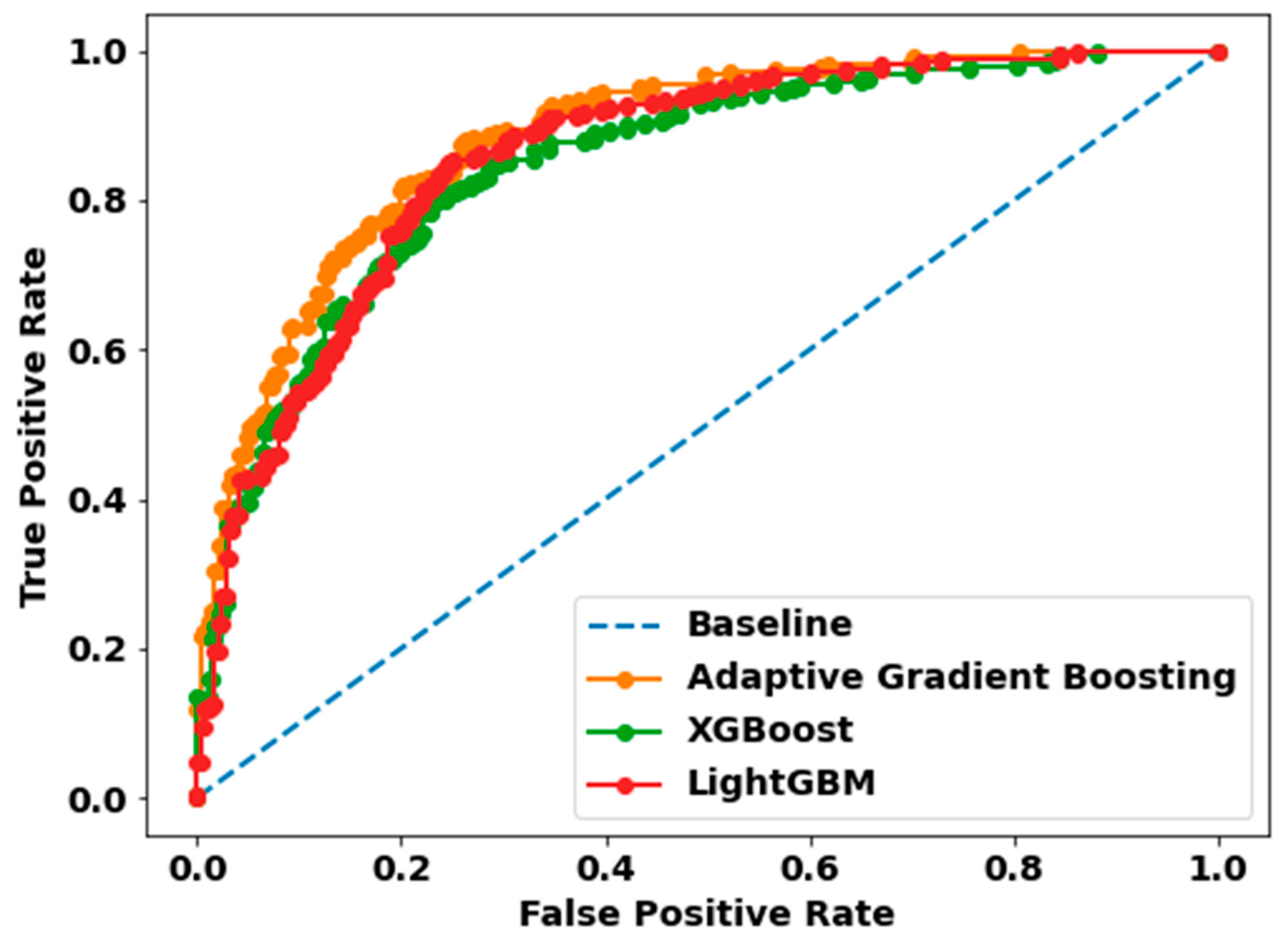
| Model | Precision | Recall | F1-Score | Accuracy | AUC |
|---|---|---|---|---|---|
| Adaptive Gradient Boosting | 0.82 | 0.78 | 0.80 | 0.80 | 0.80 |
| XGBoost | 0.79 | 0.74 | 0.77 | 0.77 | 0.77 |
| LightGBM | 0.80 | 0.76 | 0.78 | 0.78 | 0.78 |
Publisher’s Note: MDPI stays neutral with regard to jurisdictional claims in published maps and institutional affiliations. |
© 2022 by the authors. Licensee MDPI, Basel, Switzerland. This article is an open access article distributed under the terms and conditions of the Creative Commons Attribution (CC BY) license (https://creativecommons.org/licenses/by/4.0/).
Share and Cite
Islam, M.S.; Hussain, I.; Rahman, M.M.; Park, S.J.; Hossain, M.A. Explainable Artificial Intelligence Model for Stroke Prediction Using EEG Signal. Sensors 2022, 22, 9859. https://doi.org/10.3390/s22249859
Islam MS, Hussain I, Rahman MM, Park SJ, Hossain MA. Explainable Artificial Intelligence Model for Stroke Prediction Using EEG Signal. Sensors. 2022; 22(24):9859. https://doi.org/10.3390/s22249859
Chicago/Turabian StyleIslam, Mohammed Saidul, Iqram Hussain, Md Mezbaur Rahman, Se Jin Park, and Md Azam Hossain. 2022. "Explainable Artificial Intelligence Model for Stroke Prediction Using EEG Signal" Sensors 22, no. 24: 9859. https://doi.org/10.3390/s22249859