
A Tiled Ultrasound Matrix Transducer for Volumetric Imaging of the Carotid Artery
 , ,
, ,  , , , , and
Abstract
:1. Introduction
2. Materials and Methods
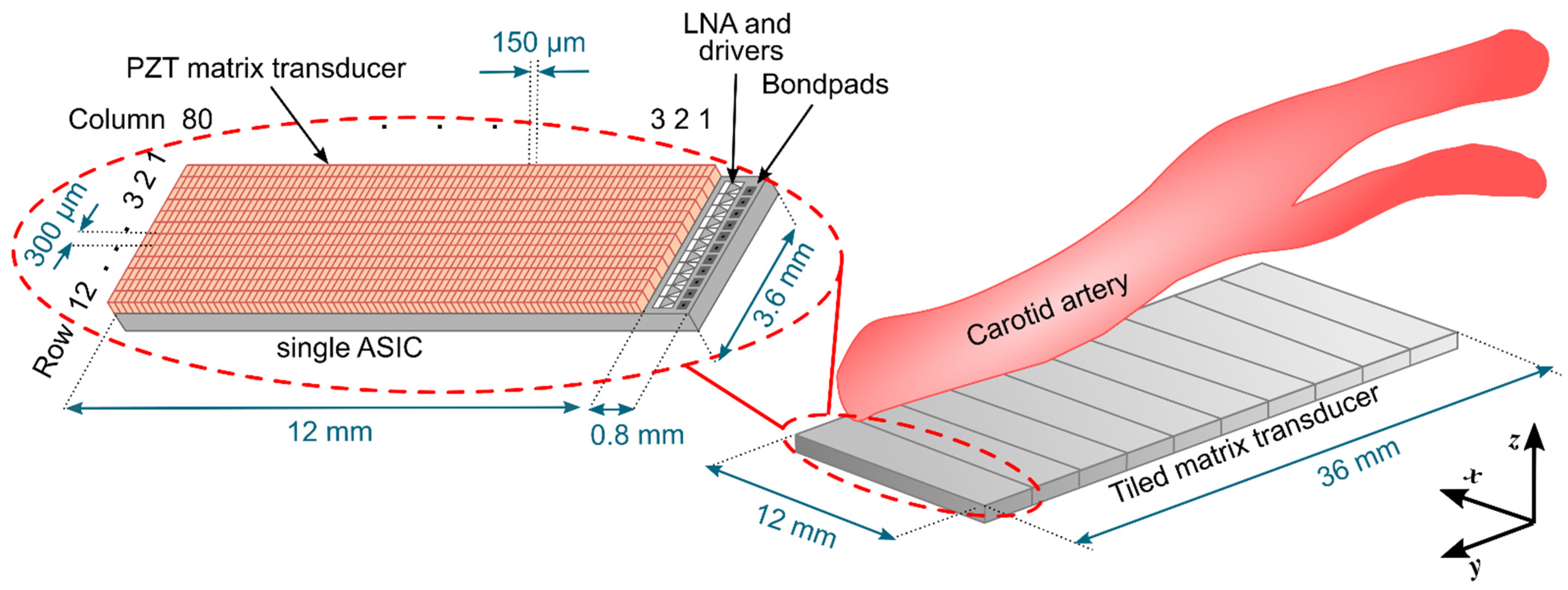
2.1. Design Choices
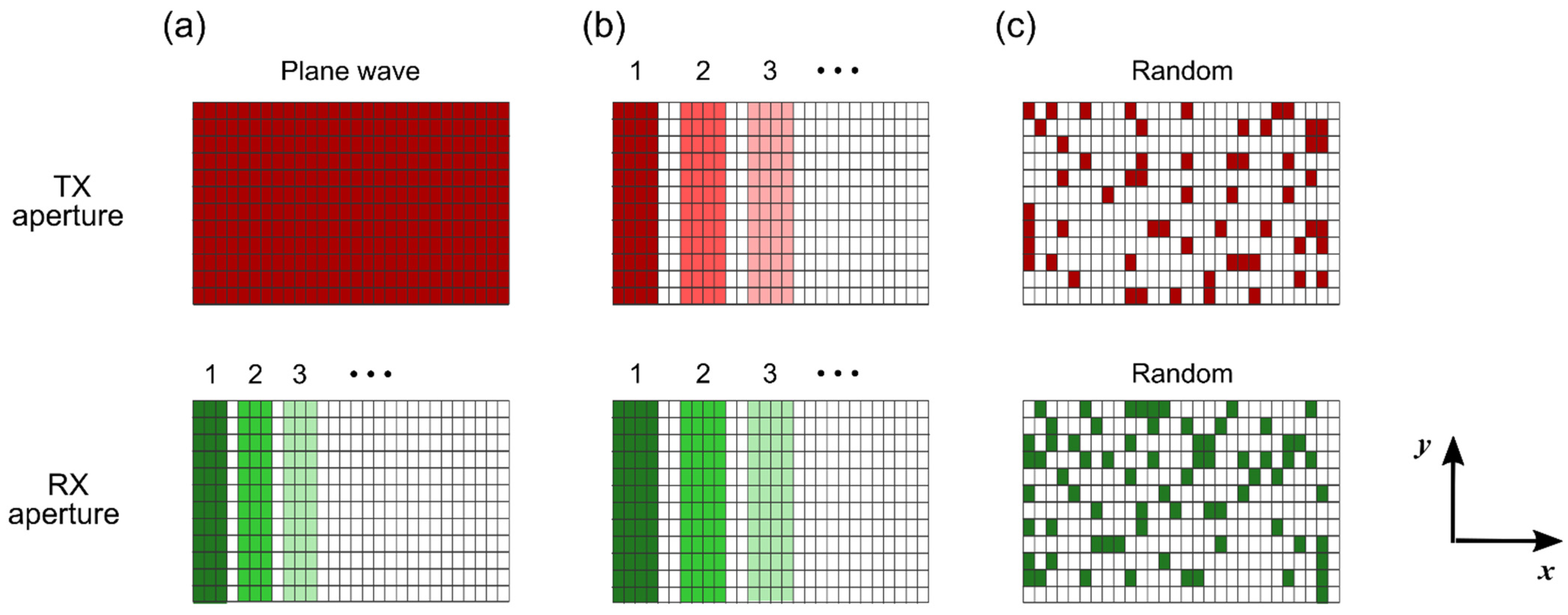
2.2. Imaging Scheme
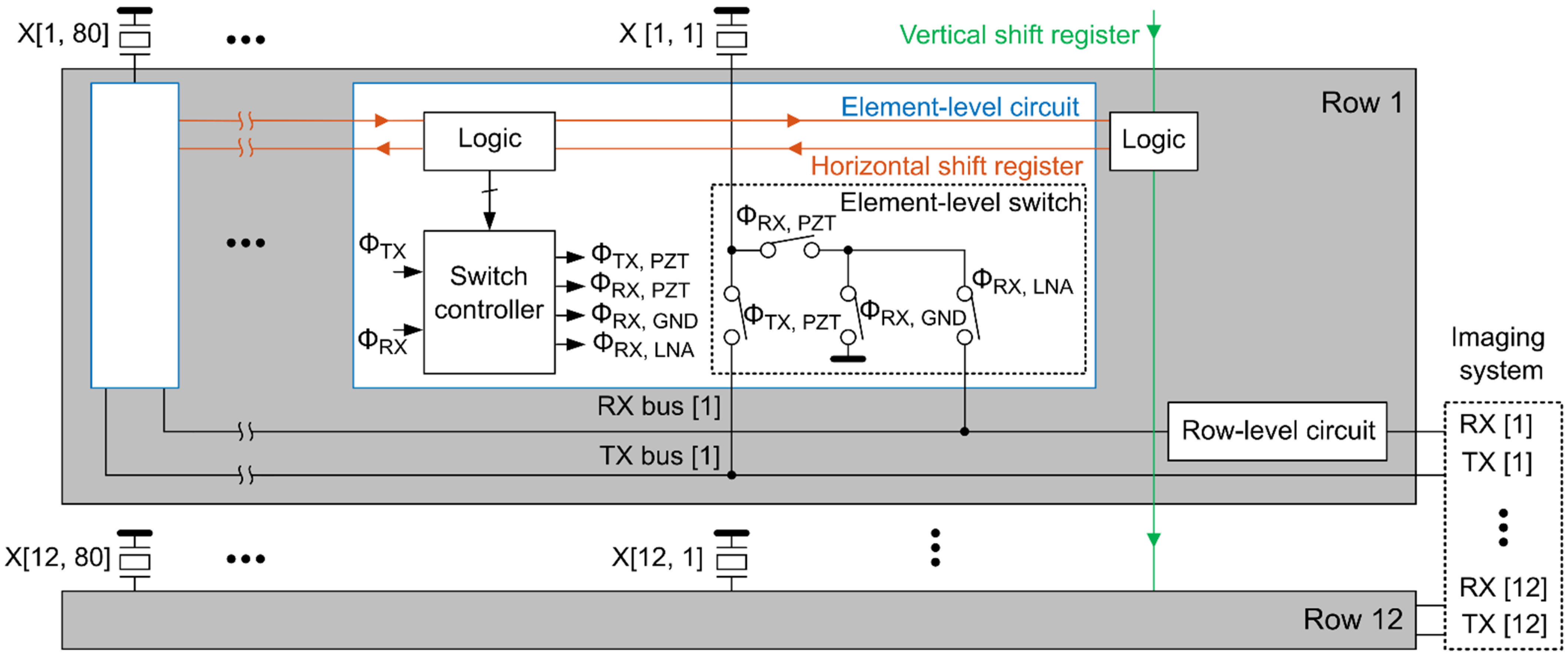
2.3. ASIC Design and Implementation
2.4. Acoustic Stack Design and Fabrication
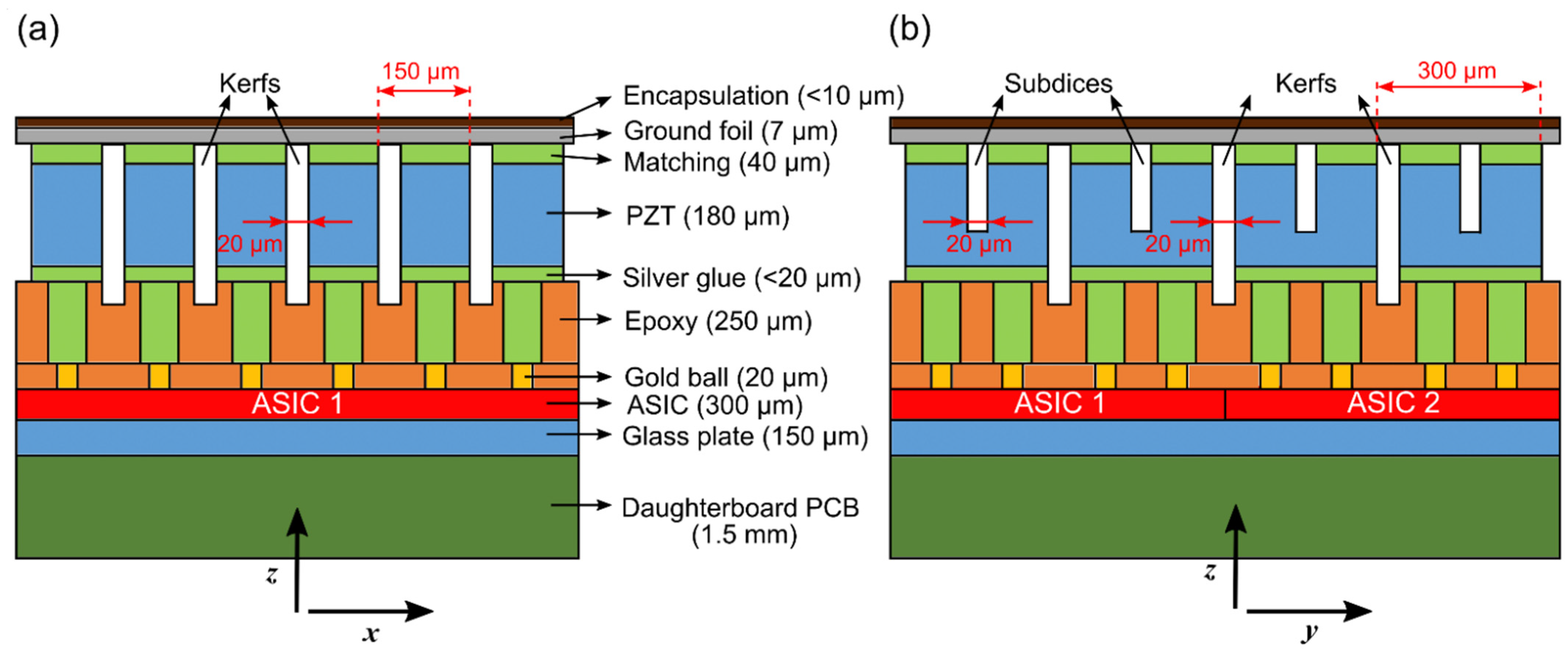
2.4.1. Stack Design
2.4.2. Stack Fabrication
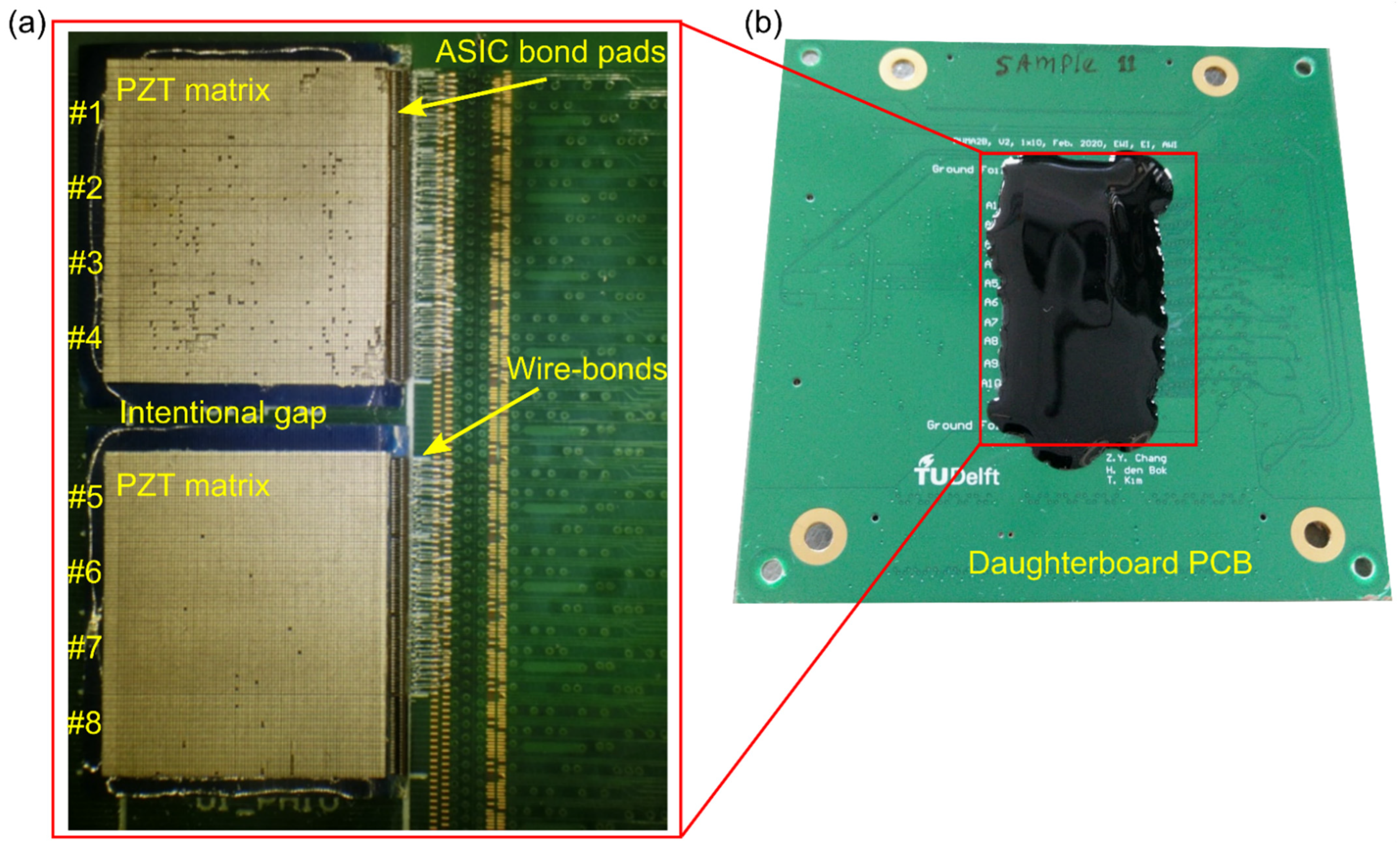
2.4.3. Electrical Connections
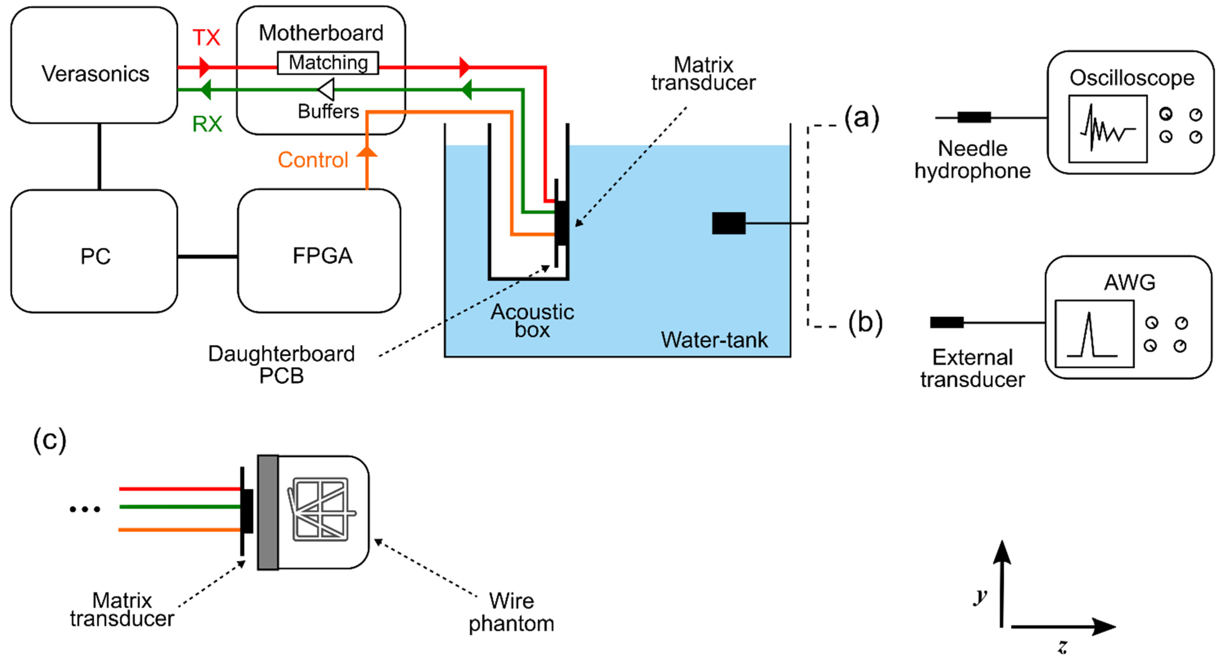
2.5. Measurement Setup
2.5.1. Electrical Characterization
2.5.2. Acoustical Characterization
2.5.3. Imaging
3. Results
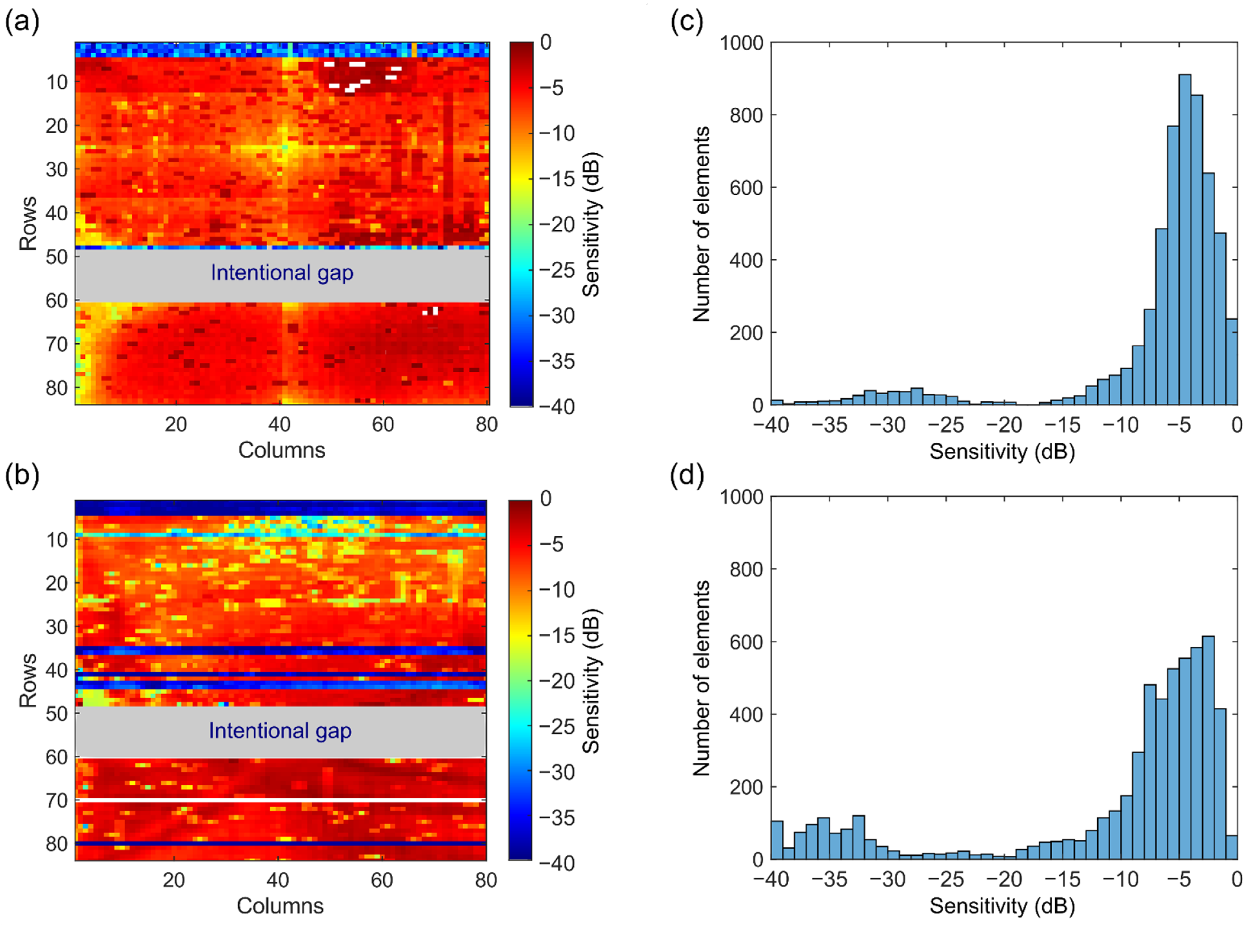
3.1. Sensitivity
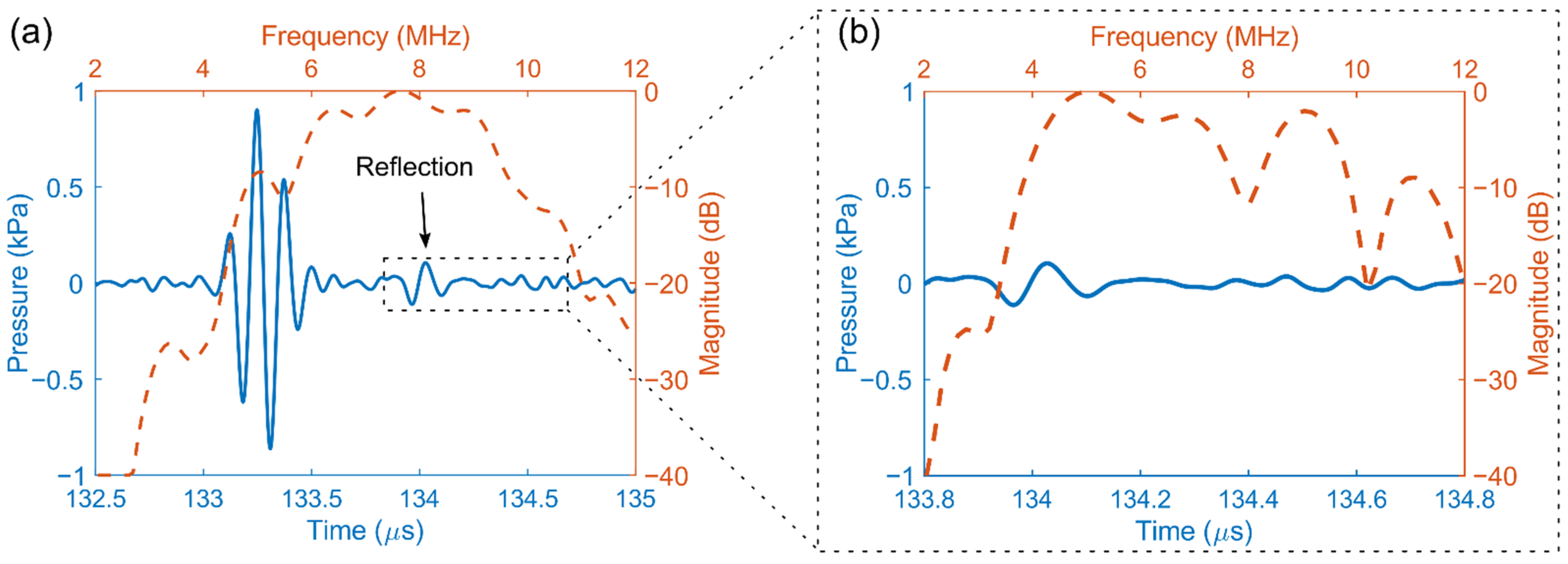
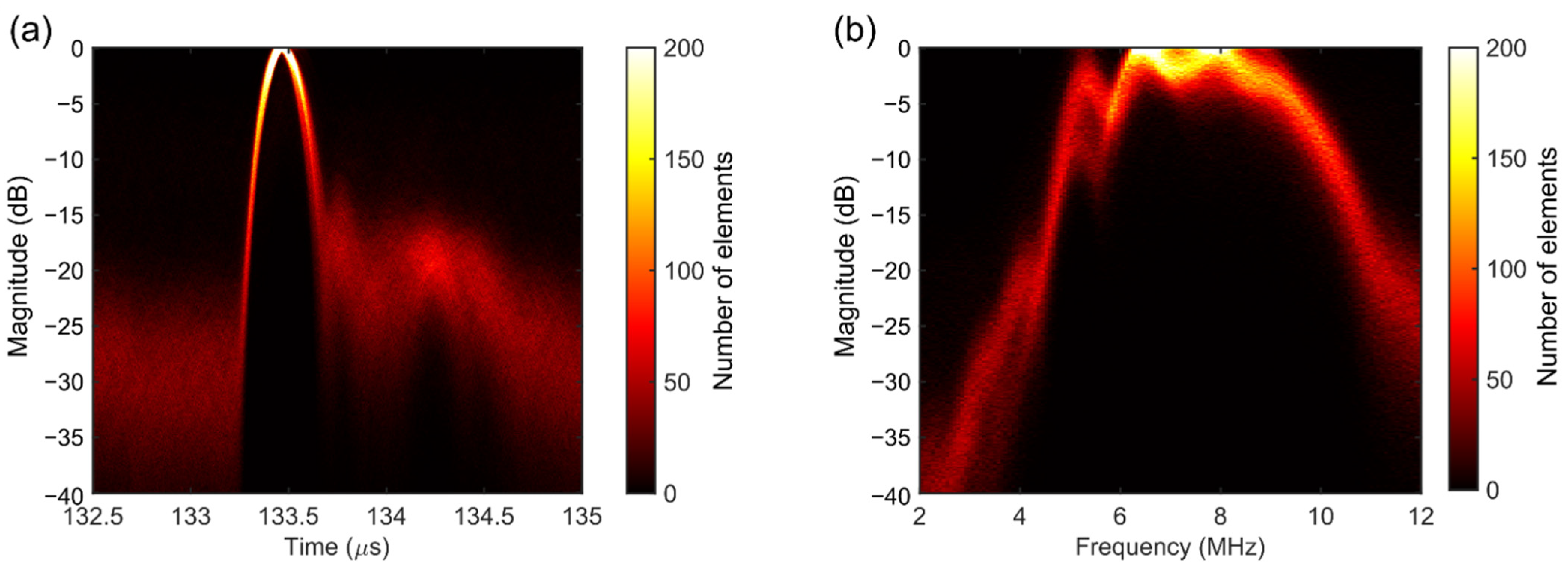
3.2. Time and Frequency Response
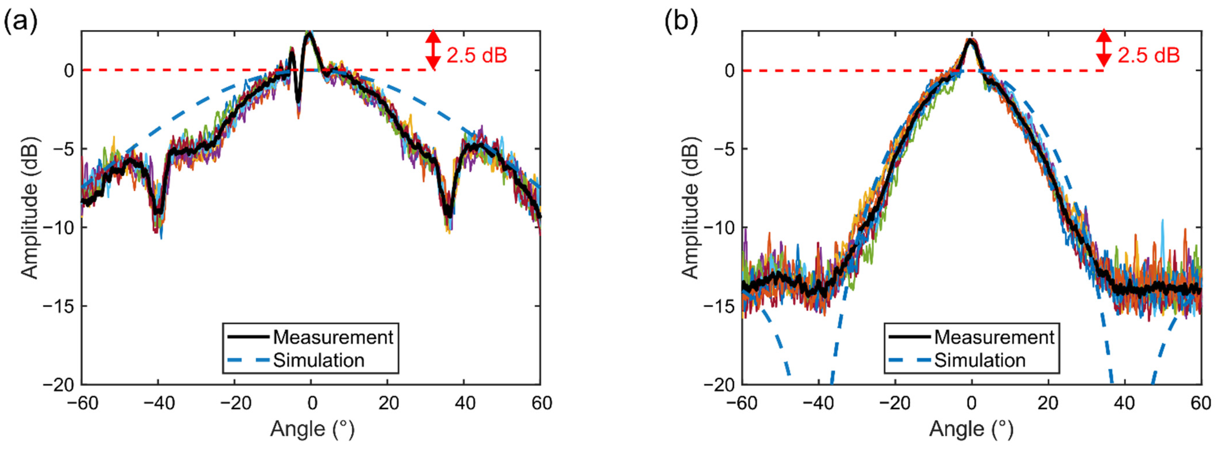
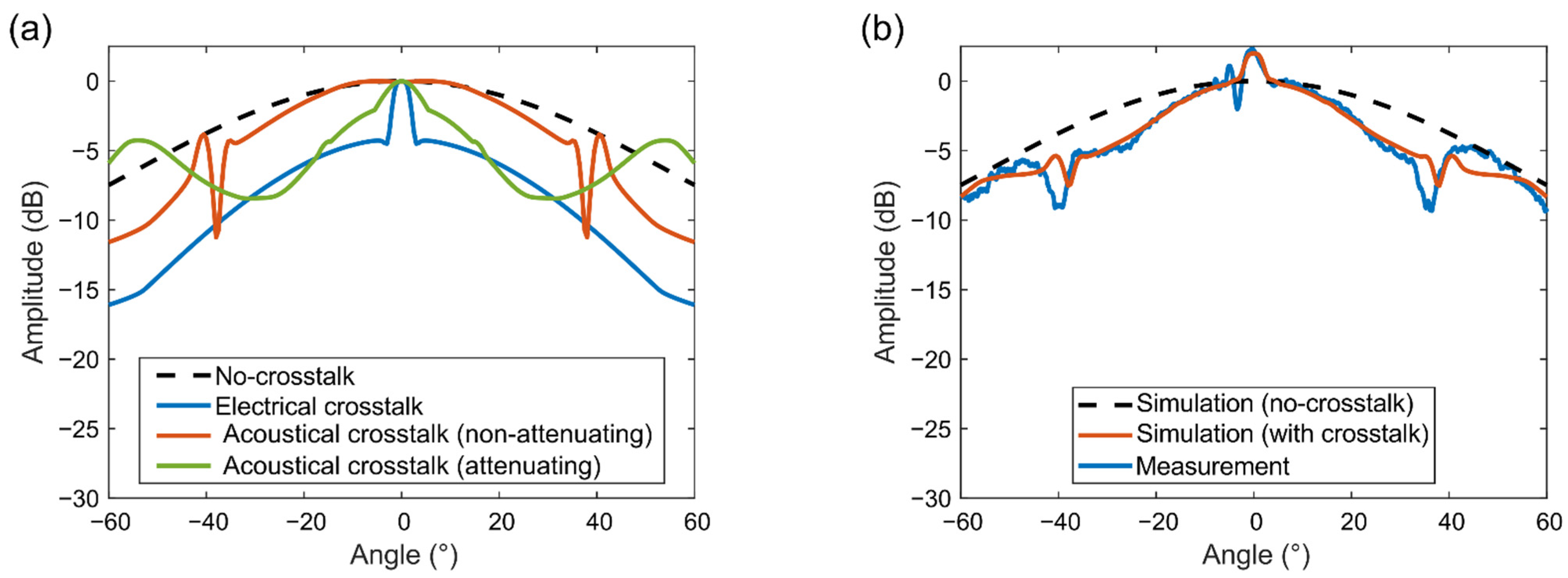
3.3. Directivity Pattern
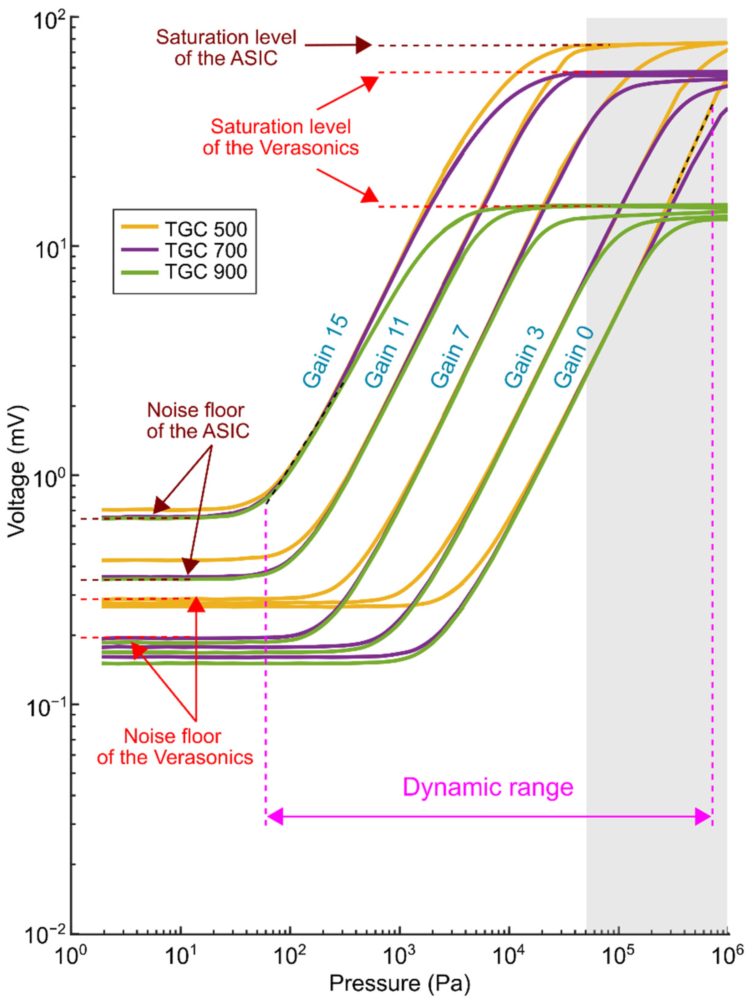
3.4. Dynamic Range
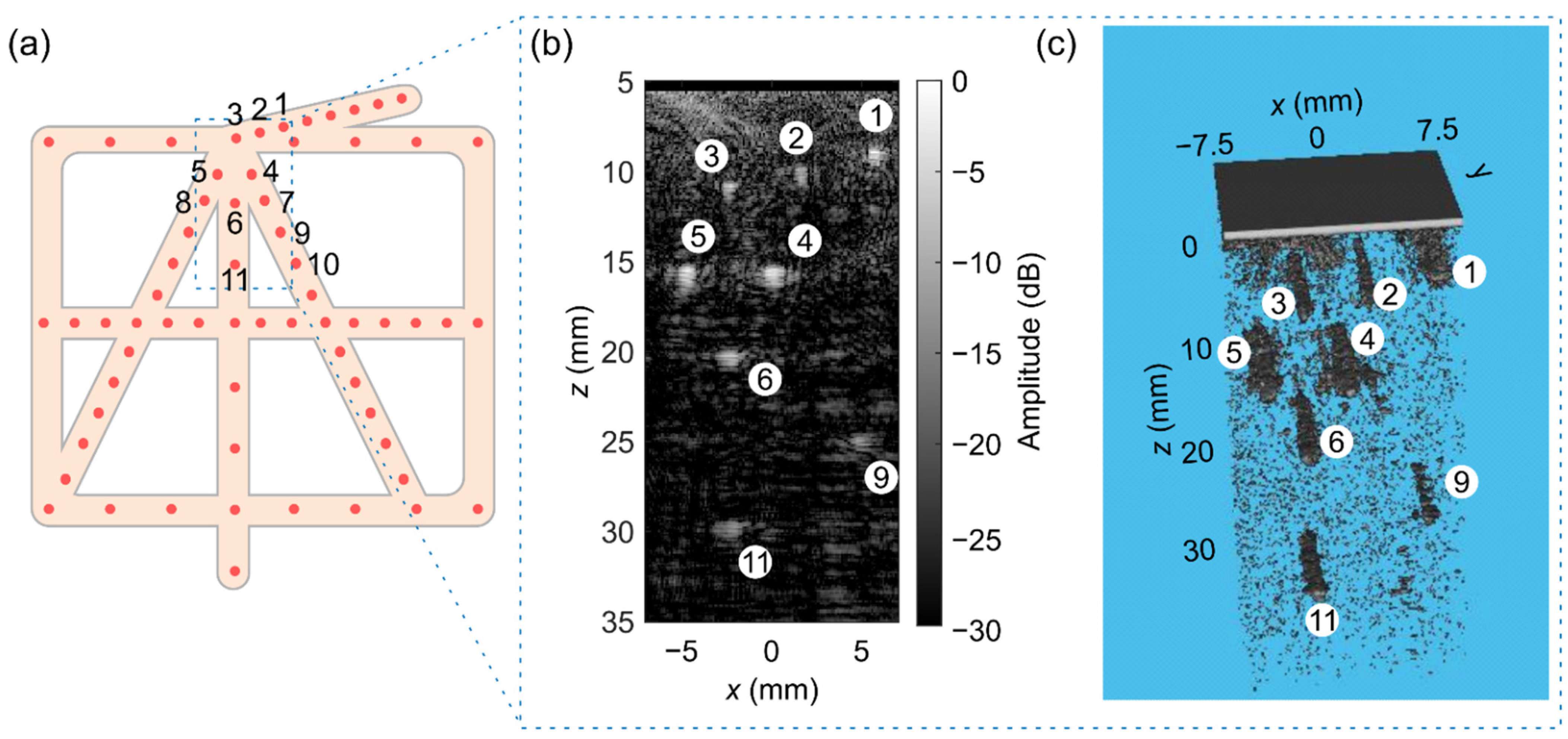
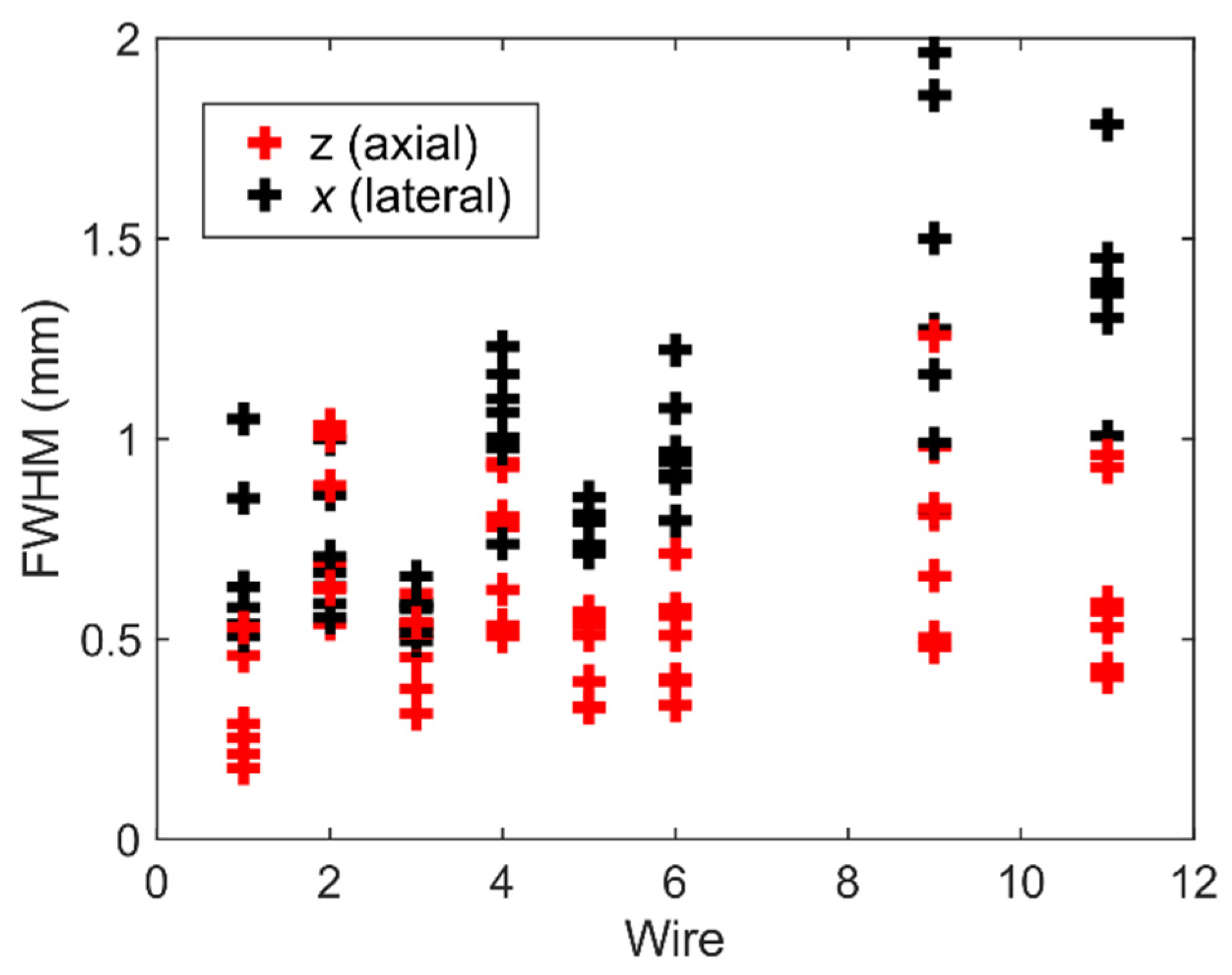
3.5. Imaging
4. Discussion
5. Conclusions
Author Contributions
Funding
Institutional Review Board Statement
Informed Consent Statement
Data Availability Statement
Conflicts of Interest
Appendix A. Electrical Characterization


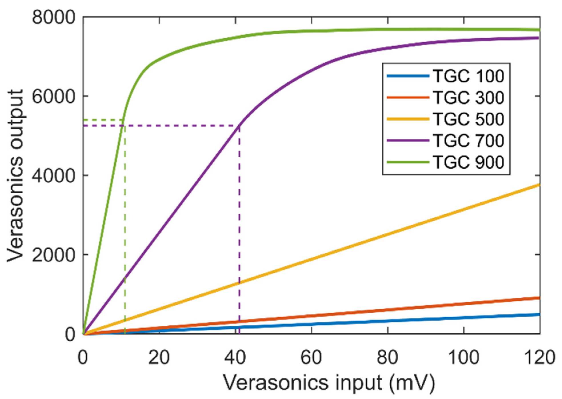
| TGC | Maximum Input (mV) | Verasonics Output | Slope (1/mV) |
|---|---|---|---|
| 100 | 310 | 1245 | 4.1 |
| 300 | 310 | 2315 | 7.6 |
| 500 | 185 | 5497 | 31.4 |
| 700 | 45 | 5514 | 129.3 |
| 900 | 11 | 5602 | 543.3 |
Appendix B. Crosstalk Analysis


| Electrical | Acoustical (Non-Attenuating) | Acoustical (Attenuating) | |
|---|---|---|---|
| Amplitude | −30 dB | −20 dB | −3.5 dB * |
| Time delay * | - | 0.0612 µs | 0.0833 µs |
| Propagation speed | - | 2450 m/s | 1800 m/s |
References
- Dakok, K.K.; Matjafri, M.Z.; Suardi, N.; Oglat, A.A.; Nabasu, S.E. A Review of Carotid Artery Phantoms for Doppler Ultrasound Applications. J. Med. Ultrasound 2021, 29, 157–166. [Google Scholar] [CrossRef]
- Delcker, A.; Tegeler, C. Influence of ECG-Triggered Data Acquisition on Reliability for Carotid Plaque Volume Measurements with a Magnetic Sensor Three-Dimensional Ultrasound System. Ultrasound Med. Biol. 1998, 24, 601–605. [Google Scholar] [CrossRef]
- Kruizinga, P.; Mastik, F.; de Jong, N.; van der Steen, A.F.W.; van Soest, G. High Frame Rate Ultrasound Imaging of Human Carotid Artery Dynamics. In Proceedings of the 2012 IEEE International Ultrasonics Symposium, Dresden, Germany, 7–10 October 2012; pp. 1177–1180. [Google Scholar]
- Landry, A.; Spence, J.D.; Fenster, A. Measurement of Carotid Plaque Volume by 3-Dimensional Ultrasound. Stroke 2004, 35, 864–869. [Google Scholar] [CrossRef] [Green Version]
- Spence, J.D.; Eliasziw, M.; DiCicco, M.; Hackam, D.G.; Galil, R.; Lohmann, T. Carotid Plaque Area. Stroke 2002, 33, 2916–2922. [Google Scholar] [CrossRef] [Green Version]
- Fenster, A.; Downey, D.B.; Cardinal, H.N. Three-Dimensional Ultrasound Imaging. Phys. Med. Biol. 2001, 46, R67–R99. [Google Scholar] [CrossRef]
- Prager, R.W.; Ijaz, U.Z.; Gee, A.H.; Treece, G.M. Three-Dimensional Ultrasound Imaging. Proc. Inst. Mech. Eng. Part H J. Eng. Med. 2010, 224, 193–223. [Google Scholar] [CrossRef]
- Schminke, U.; Motsch, L.; Griewing, B.; Gaull, M.; Kessler, C. Three-Dimensional Power-Mode Ultrasound for Quantification of the Progression of Carotid Artery Atherosclerosis. J. Neurol. 2000, 247, 106–111. [Google Scholar] [CrossRef]
- Delcker, A.; Diener, H.C. Quantification of Atherosclerotic Plaques in Carotid Arteries by Three-Dimensional Ultrasound. Br. J. Radiol. 1994, 67, 672–678. [Google Scholar] [CrossRef]
- Harloff, A. Carotid Plaque Hemodynamics. Interv. Neurol. 2012, 1, 44–54. [Google Scholar] [CrossRef]
- Holbek, S.; Pihl, M.J.; Ewertsen, C.; Nielsen, M.B.; Jensen, J.A. In Vivo 3-D Vector Velocity Estimation with Continuous Data. In Proceedings of the 2015 IEEE International Ultrasonics Symposium (IUS), Taipei, Taiwan, 21–24 October 2015; pp. 1–4. [Google Scholar]
- Provost, J.; Papadacci, C.; Arango, J.E.; Imbault, M.; Fink, M.; Gennisson, J.L.; Tanter, M.; Pernot, M. 3D Ultrafast Ultrasound Imaging in Vivo. Phys. Med. Biol. 2014, 59, L1–L13. [Google Scholar] [CrossRef]
- Heiles, B.; Correia, M.; Hingot, V.; Pernot, M.; Provost, J.; Tanter, M.; Couture, O. Ultrafast 3D Ultrasound Localization Microscopy Using a 32 × 32 Matrix Array. IEEE Trans. Med. Imaging 2019, 38, 2005–2015. [Google Scholar] [CrossRef]
- Mozaffarzadeh, M.; Soozande, M.; Fool, F.; Pertijs, M.A.P.; Vos, H.J.; Verweij, M.D.; Bosch, J.G.; de Jong, N. Receive/Transmit Aperture Selection for 3D Ultrasound Imaging with a 2D Matrix Transducer. Appl. Sci. 2020, 10, 5300. [Google Scholar] [CrossRef]
- Kim, T.; Fool, F.; dos Santos, D.S.; Chang, Z.-Y.; Noothout, E.; Vos, H.J.; Bosch, J.G.; Verweij, M.D.; de Jong, N.; Pertijs, M.A.P. Design of an Ultrasound Transceiver ASIC with a Switching-Artifact Reduction Technique for 3D Carotid Artery Imaging. Sensors 2020, 21, 150. [Google Scholar] [CrossRef]
- Roux, E.; Ramalli, A.; Robini, M.; Liebgott, H.; Cachard, C.; Tortoli, P. Spiral Array Inspired Multi-Depth Cost Function for 2D Sparse Array Optimization. In Proceedings of the 2015 IEEE International Ultrasonics Symposium (IUS), Taipei, Taiwan, 21–24 October 2015; pp. 1–4. [Google Scholar]
- Ellens, N.; Pulkkinen, A.; Song, J.; Hynynen, K. The Utility of Sparse 2D Fully Electronically Steerable Focused Ultrasound Phased Arrays for Thermal Surgery: A Simulation Study. Phys. Med. Biol. 2011, 56, 4913–4932. [Google Scholar] [CrossRef]
- Ramaekers, P.; de Greef, M.; Berriet, R.; Moonen, C.T.W.; Ries, M. Evaluation of a Novel Therapeutic Focused Ultrasound Transducer Based on Fermat’s Spiral. Phys. Med. Biol. 2017, 62, 5021–5045. [Google Scholar] [CrossRef]
- Ramalli, A.; Boni, E.; Savoia, A.S.; Tortoli, P. Density-Tapered Spiral Arrays for Ultrasound 3-D Imaging. IEEE Trans. Ultrason. Ferroelectr. Freq. Control 2015, 62, 1580–1588. [Google Scholar] [CrossRef]
- Wygant, I.O.; Jamal, N.S.; Lee, H.J.; Nikoozadeh, A.; Oralkan, O.; Karaman, M.; Khuri-yakub, B.T. An Integrated Circuit with Transmit Beamforming Flip-Chip Bonded to a 2-D CMUT Array for 3-D Ultrasound Imaging. IEEE Trans. Ultrason. Ferroelectr. Freq. Control 2009, 56, 2145–2156. [Google Scholar] [CrossRef]
- Wei, L.; Wahyulaksana, G.; Meijlink, B.; Ramalli, A.; Noothout, E.; Verweij, M.D.; Boni, E.; Kooiman, K.; Van Der Steen, A.F.W.; Tortoli, P.; et al. High Frame Rate Volumetric Imaging of Microbubbles Using a Sparse Array and Spatial Coherence Beamforming. IEEE Trans. Ultrason. Ferroelectr. Freq. Control 2021, 68, 3069–3081. [Google Scholar] [CrossRef]
- Roux, E.; Varray, F.; Petrusca, L.; Cachard, C.; Tortoli, P.; Liebgott, H. Experimental 3-D Ultrasound Imaging with 2-D Sparse Arrays Using Focused and Diverging Waves. Sci. Rep. 2018, 8, 1–12. [Google Scholar] [CrossRef] [Green Version]
- Rasmussen, M.F.; Jensen, J.A. 3-D Ultrasound Imaging Performance of a Row-Column Addressed 2-D Array Transducer: A Measurement Study. In Proceedings of the 2013 IEEE International Ultrasonics Symposium (IUS), Prague, Czech Republic, 21–25 July 2013; pp. 1460–1463. [Google Scholar]
- Chen, K.; Lee, H.S.; Sodini, C.G. A Column-Row-Parallel ASIC Architecture for 3-D Portable Medical Ultrasonic Imaging. IEEE J. Solid-State Circuits 2016, 51, 738–751. [Google Scholar] [CrossRef]
- Flesch, M.; Pernot, M.; Provost, J.; Ferin, G.; Nguyen-Dinh, A.; Tanter, M.; Deffieux, T. 4D In Vivo Ultrafast Ultrasound Imaging Using a Row-Column Addressed Matrix and Coherently-Compounded Orthogonal Plane Waves. Phys. Med. Biol. 2017, 62, 4571–4588. [Google Scholar] [CrossRef]
- Janjic, J.; Tan, M.; Daeichin, V.; Noothout, E.; Chen, C.; Chen, Z.; Chang, Z.Y.; Beurskens, R.H.S.H.; Van Soest, G.; Van Der Steen, A.F.W.; et al. A 2-D Ultrasound Transducer with Front-End ASIC and Low Cable Count for 3-D Forward-Looking Intravascular Imaging: Performance and Characterization. IEEE Trans. Ultrason. Ferroelectr. Freq. Control 2018, 65, 1832–1844. [Google Scholar] [CrossRef] [Green Version]
- Wildes, D.; Lee, W.; Haider, B.; Cogan, S.; Sundaresan, K.; Mills, D.M.; Yetter, C.; Hart, P.H.; Haun, C.R.; Concepcion, M.; et al. 4-D ICE: A 2-D Array Transducer with Integrated ASIC in a 10-Fr Catheter for Real-Time 3-D Intracardiac Echocardiography. IEEE Trans. Ultrason. Ferroelectr. Freq. Control. 2016, 63, 2159–2173. [Google Scholar] [CrossRef]
- Savord, B.; Solomon, R. Fully Sampled Matrix Transducer for Real Time 3D Ultrasonic Imaging. Proc. IEEE Ultrason. Symp. 2003, 1, 945–953. [Google Scholar] [CrossRef]
- Chen, C.; Chen, Z.; Bera, D.; Noothout, E.; Chang, Z.-Y.; Tan, M.; Vos, H.J.; Bosch, J.G.; Verweij, M.D.; de Jong, N.; et al. A Pitch-Matched Front-End ASIC With Integrated Subarray Beamforming ADC for Miniature 3-D Ultrasound Probes. IEEE J. Solid-State Circuits 2018, 53, 3050–3064. [Google Scholar] [CrossRef]
- Carpenter, T.M.; Rashid, M.W.; Ghovanloo, M.; Cowell, D.M.J.; Freear, S.; Degertekin, F.L. Direct Digital Demultiplexing of Analog TDM Signals for Cable Reduction in Ultrasound Imaging Catheters. IEEE Trans. Ultrason. Ferroelectr. Freq. Control 2016, 63, 1078–1085. [Google Scholar] [CrossRef] [Green Version]
- Kang, E.; Ding, Q.; Shabanimotlagh, M.; Kruizinga, P.; Chang, Z.-Y.; Noothout, E.; Vos, H.J.; Bosch, J.G.; Verweij, M.D.; de Jong, N.; et al. A Reconfigurable Ultrasound Transceiver ASIC With 24 × 40 Elements for 3-D Carotid Artery Imaging. IEEE J. Solid-State Circuits 2018, 53, 2065–2075. [Google Scholar] [CrossRef] [Green Version]
- Chen, C.; Chen, Z.; Bera, D.; Raghunathan, S.B.; Shabanimotlagh, M.; Noothout, E.; Chang, Z.Y.; Ponte, J.; Prins, C.; Vos, H.J.; et al. A Front-End ASIC with Receive Sub-Array Beamforming Integrated with a 32 × 32 PZT Matrix Transducer for 3-D Transesophageal Echocardiography. IEEE J. Solid-State Circuits 2017, 52, 994–1006. [Google Scholar] [CrossRef] [Green Version]
- Philips. The XMATRIX Transducer Technology. Available online: https://www.usa.philips.com/healthcare/resources/feature-detail/xmatrix/ (accessed on 28 July 2022).
- Butterfly. New Butterfly IQ+. Available online: https://www.butterflynetwork.eu/ (accessed on 14 September 2022).
- Rothberg, J.M.; Ralston, T.S.; Rothberg, A.G.; Martin, J.; Zahorian, J.S.; Alie, S.A.; Sanchez, N.J.; Chen, K.; Chen, C.; Thiele, K.; et al. Ultrasound-on-Chip Platform for Medical Imaging, Analysis, and Collective Intelligence. Proc. Natl. Acad. Sci. USA 2021, 118, e2019339118. [Google Scholar] [CrossRef]
- Fujifilm. Technologies. Available online: https://hce.fujifilm.com/products/ultrasound/technologies.html (accessed on 14 September 2022).
- Fool, F.; Verweij, M.D.; Vos, H.J.; Shabanimotlagh, M.; Soozande, M.; Mozaffarzadeh, M.; Kim, T.; Kang, E.; Pertijs, M.; Jong, N. De 3D High Frame Rate Flow Measurement Using a Prototype Matrix Transducer for Carotid Imaging. In Proceedings of the 2019 IEEE International Ultrasonics Symposium (IUS), Glasgow, UK, 6–9 October 2019; pp. 2242–2245. [Google Scholar]
- Tahmasebpour, H.R.; Buckley, A.R.; Cooperberg, P.L.; Fix, C.H. Sonographic Examination of the Carotid Arteries. Radiographics 2005, 25, 1561–1575. [Google Scholar] [CrossRef]
- Nguyen, H.-V.; Eggen, T.; Sten-Nilsen, B.; Imenes, K.; Aasmundtveit, K.E. Assembly of Multiple Chips on Flexible Substrate Using Anisotropie Conductive Film for Medical Imaging Applications. In Proceedings of the 2014 IEEE 64th Electronic Components and Technology Conference (ECTC), Lake Buena Vista, FL, USA, 27–30 May 2014; pp. 498–503. [Google Scholar]
- Boni, E.; Bassi, L.; Dallai, A.; Guidi, F.; Meacci, V.; Ramalli, A.; Ricci, S.; Tortoli, P. ULA-OP 256: A 256-Channel Open Scanner for Development and Real-Time Implementation of New Ultrasound Methods. IEEE Trans. Ultrason. Ferroelectr. Freq. Control 2016, 63, 1488–1495. [Google Scholar] [CrossRef]
- Verasonics. The Vantage System. Available online: https://verasonics.com/the-vantage-advantage/ (accessed on 5 May 2022).
- de Jong, N.; Bom, N.; Souquet, J.; Faber, G. Vibration Modes, Matching Layers and Grating Lobes. Ultrasonics 1985, 23, 176–182. [Google Scholar] [CrossRef]
- Janjic, J.; Shabanimotlagh, M.; van Soest, G.; van der Steen, A.F.W.; de Jong, N.; Verweij, M.D. Improving the Performance of a 1-D Ultrasound Transducer Array by Subdicing. IEEE Trans. Ultrason. Ferroelectr. Freq. Control 2016, 63, 1161–1171. [Google Scholar] [CrossRef]
- dos Santos, D.S.; Fool, F.; Kim, T.; Noothout, E.; Vos, H.J.; Bosch, J.G.; Pertijs, M.A.P.; Verweij, M.D.; de Jong, N. Experimental Investigation of the Effect of Subdicing on an Ultrasound Matrix Transducer. In Proceedings of the 2021 IEEE International Ultrasonics Symposium (IUS), Xi’an, China, 11 September 2021; pp. 1–3. [Google Scholar]
- Tortoli, P.; Lenge, M.; Righi, D.; Ciuti, G.; Liebgott, H.; Ricci, S. Comparison of Carotid Artery Blood Velocity Measurements by Vector and Standard Doppler Approaches. Ultrasound Med. Biol. 2015, 41, 1354–1362. [Google Scholar] [CrossRef]
- Kruizinga, P.; Kang, E.; Shabanimotlagh, M.; Ding, Q.; Noothout, E.; Chang, Z.Y.; Vos, H.J.; Bosch, J.G.; Verweij, M.D.; Pertijs, M.A.P.; et al. Towards 3D Ultrasound Imaging of the Carotid Artery Using a Programmable and Tileable Matrix Array. In Proceedings of the 2017 IEEE International Ultrasonics Symposium (IUS), Washington, DC, USA, 6–9 September 2017; pp. 1–3. [Google Scholar]
- Shabanimotlagh, M.; Daeichin, V.; Raghunathan, S.B.; Kruizinga, P.; Vos, H.J.; Bosch, J.G.; Pertijs, M.; De Jong, N.; Verweij, M. Optimizing the Directivity of Piezoelectric Matrix Transducer Elements Mounted on an ASIC. In Proceedings of the 2017 IEEE International Ultrasonics Symposium (IUS), Washington, DC, USA, 6–9 September 2017; pp. 1–4. [Google Scholar] [CrossRef]
- Lee, S.; Choi, K.; Lee, K.; Kim, Y.; Park, S. A Quarter-Wavelength Vibration Mode Transducer Using Clamped Boundary Backing Layer. In proceedings of the 2012 World Congress on Advances in Civil, Environmental, and Materials Research (ACEM’12), Seoul, Korea, 26–30 August 2012. pp. 1634–1639.
- Wodnicki, R.; Kang, H.; Chen, R.; Cabrera-Munoz, N.E.; Jung, H.; Jiang, L.; Foiret, J.; Liu, Y.; Chiu, V.; Stephens, D.N.; et al. Co-Integrated PIN-PMN-PT 2-D Array and Transceiver Electronics by Direct Assembly Using a 3-D Printed Interposer Grid Frame. IEEE Trans. Ultrason. Ferroelectr. Freq. Control 2020, 67, 387–401. [Google Scholar] [CrossRef]
- McGough, R.J. Rapid Calculations of Time-Harmonic Nearfield Pressures Produced by Rectangular Pistons. J. Acoust. Soc. Am. 2004, 115, 1934–1941. [Google Scholar] [CrossRef] [Green Version]
- Ranganathan, K.; Santy, M.K.; Blalock, T.N.; Hossack, J.A.; Walker, W.F. Direct Sampled I/Q Beamforming for Compact and Very Low-Cost Ultrasound Imaging. IEEE Trans. Ultrason. Ferroelectr. Freq. Control 2004, 51, 1082–1094. [Google Scholar] [CrossRef]
- Mozaffarzadeh, M.; Verschuur, E.; Verweij, M.D.; De Jong, N.; Renaud, G. Accelerated 2D Real-Time Refraction-Corrected Transcranial Ultrasound Imaging. IEEE Trans. Ultrason. Ferroelectr. Freq. Control. 2022, 69, 2599–2610. [Google Scholar] [CrossRef]
- Lynser, D.; Daniala, C.; Khan, A.Y.; Marbaniang, E.; Thangkhiew, I. Effects of Dynamic Range Variations on the Doppler Flow Velocities of Common Carotid Arteries. Artery Res. 2018, 22, 18–23. [Google Scholar] [CrossRef]
- Celmer, M.; Opieliński, K.J. Research and Modeling of Mechanical Crosstalk in Linear Arrays of Ultrasonic Transducers. Arch. Acoust. 2016, 41, 599–612. [Google Scholar] [CrossRef]
- Bybi, A.; Khouili, D.; Granger, C.; Garoum, M.; Mzerd, A.; Hladky-Hennion, A.-C. Experimental Characterization of a Piezoelectric Transducer Array Taking into Account Crosstalk Phenomenon. Int. J. Eng. Technol. Innov. 2020, 10, 1–14. [Google Scholar] [CrossRef]


| Parameter | Value |
|---|---|
| Element center frequency | 7.5 MHz |
| Element size | 300 µm × 150 µm |
| Excitation type | Hanning weighted pulse |
| Number of cycles | 1 |
| Sound speed | 1480 m/s |
| Parameter | Value |
|---|---|
| Peak pressure (kPa) | 0.6 ± 0.2 |
| Center frequency (MHz) | 7.5 ± 0.6 |
| Bandwidth −6 dB (%) | 46 ± 14 |
| Ringing time −20 dB (µs) | 0.3 ± 0.15 |
| ASIC Gain | Minimum Pressure (kPa) | Maximum Pressure (kPa) | Receive Sensitivity (µV/Pa) |
|---|---|---|---|
| 0 | 30 | 700 * | 0.06 |
| 3 | 2 | 200 * | 0.15 |
| 7 | 0.3 | 70 * | 0.72 |
| 11 | 0.2 | 20 | 2.73 |
| 15 | 0.06 | 4 | 8.79 |
Publisher’s Note: MDPI stays neutral with regard to jurisdictional claims in published maps and institutional affiliations. |
© 2022 by the authors. Licensee MDPI, Basel, Switzerland. This article is an open access article distributed under the terms and conditions of the Creative Commons Attribution (CC BY) license (https://creativecommons.org/licenses/by/4.0/).
Share and Cite
dos Santos, D.S.; Fool, F.; Mozaffarzadeh, M.; Shabanimotlagh, M.; Noothout, E.; Kim, T.; Rozsa, N.; Vos, H.J.; Bosch, J.G.; Pertijs, M.A.P.; et al. A Tiled Ultrasound Matrix Transducer for Volumetric Imaging of the Carotid Artery. Sensors 2022, 22, 9799. https://doi.org/10.3390/s22249799
dos Santos DS, Fool F, Mozaffarzadeh M, Shabanimotlagh M, Noothout E, Kim T, Rozsa N, Vos HJ, Bosch JG, Pertijs MAP, et al. A Tiled Ultrasound Matrix Transducer for Volumetric Imaging of the Carotid Artery. Sensors. 2022; 22(24):9799. https://doi.org/10.3390/s22249799
Chicago/Turabian Styledos Santos, Djalma Simões, Fabian Fool, Moein Mozaffarzadeh, Maysam Shabanimotlagh, Emile Noothout, Taehoon Kim, Nuriel Rozsa, Hendrik J. Vos, Johan G. Bosch, Michiel A. P. Pertijs, and et al. 2022. "A Tiled Ultrasound Matrix Transducer for Volumetric Imaging of the Carotid Artery" Sensors 22, no. 24: 9799. https://doi.org/10.3390/s22249799