
X-Band Radar System to Detect Bathymetric Changes at River Mouths during Storm Surges: A Case Study of the Arno River

Abstract
:1. Introduction
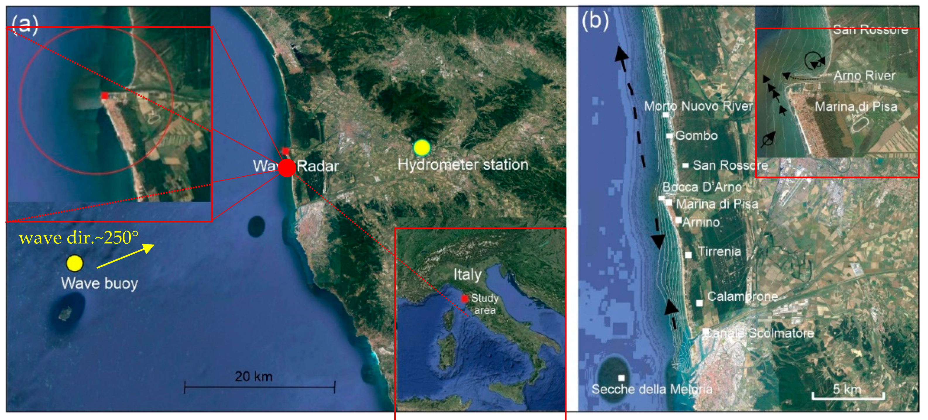
2. Study Area
3. Materials and Methods
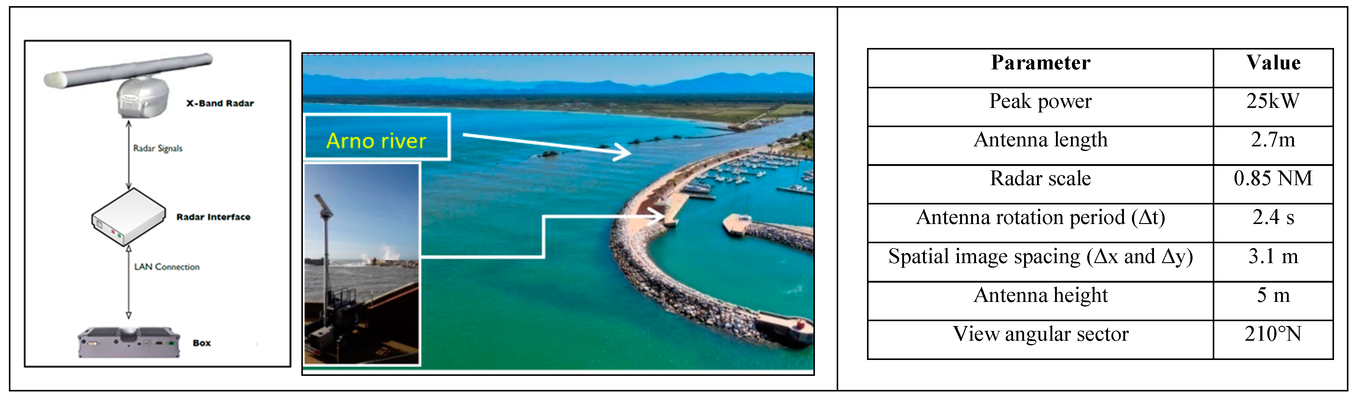
3.1. Wave Radar Systems
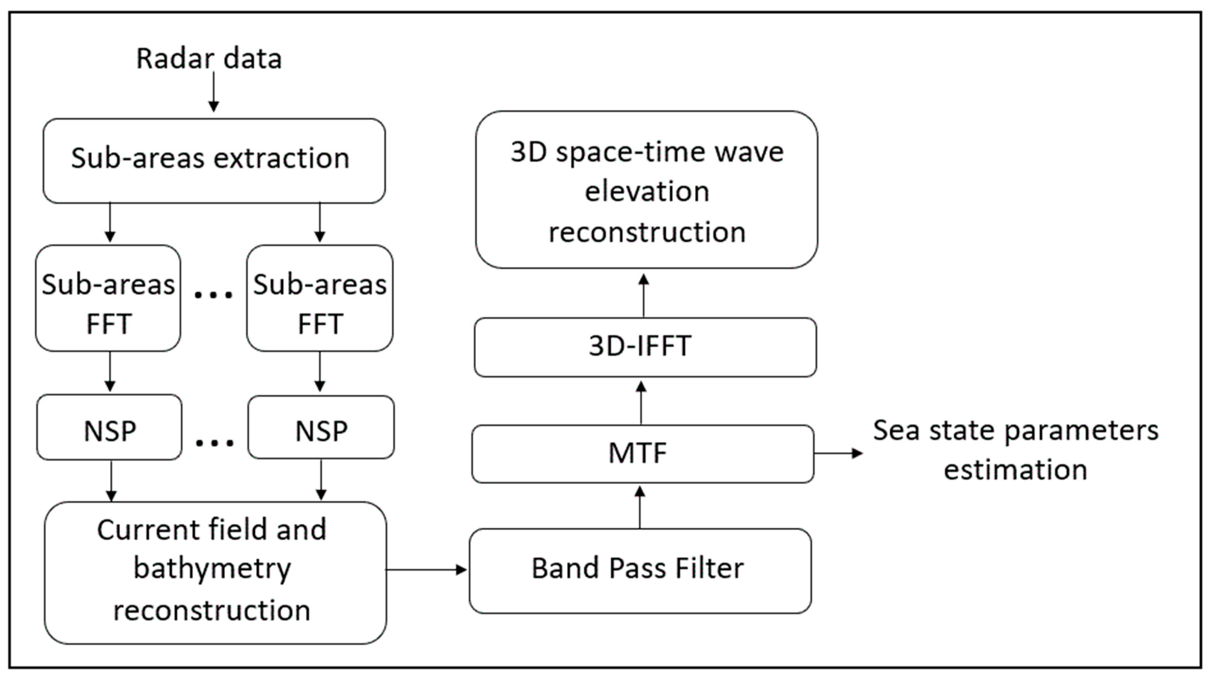
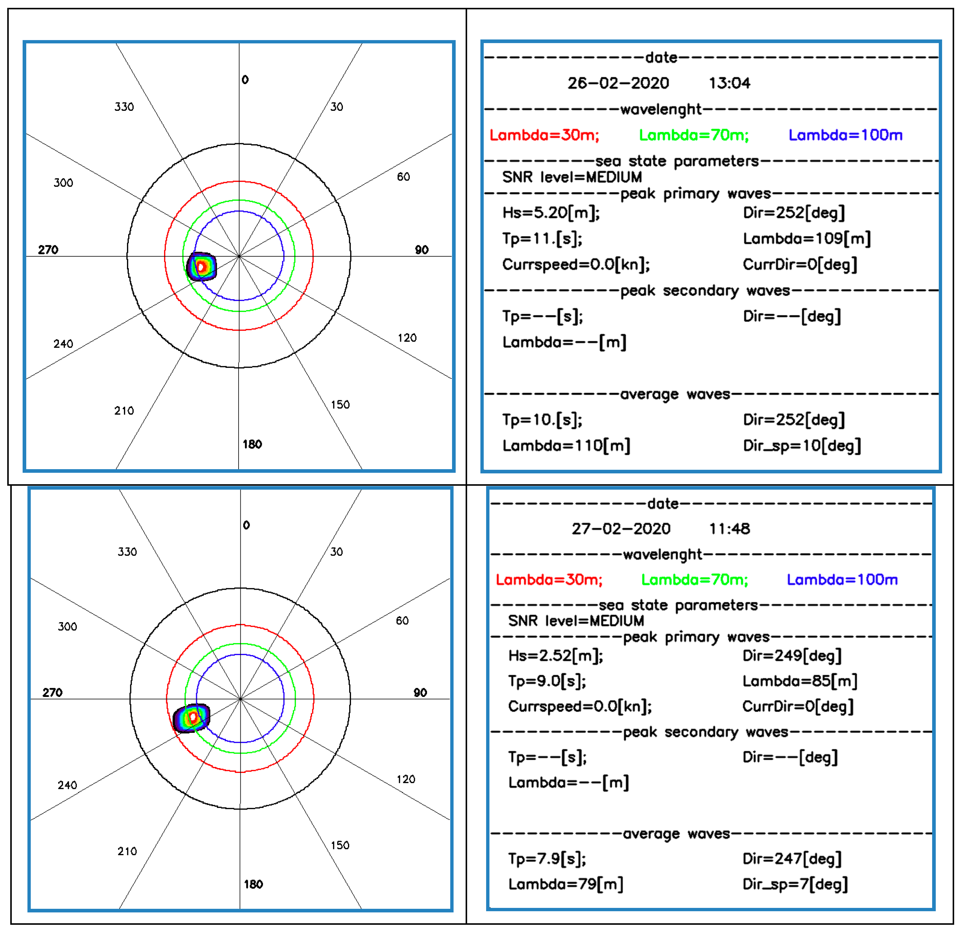
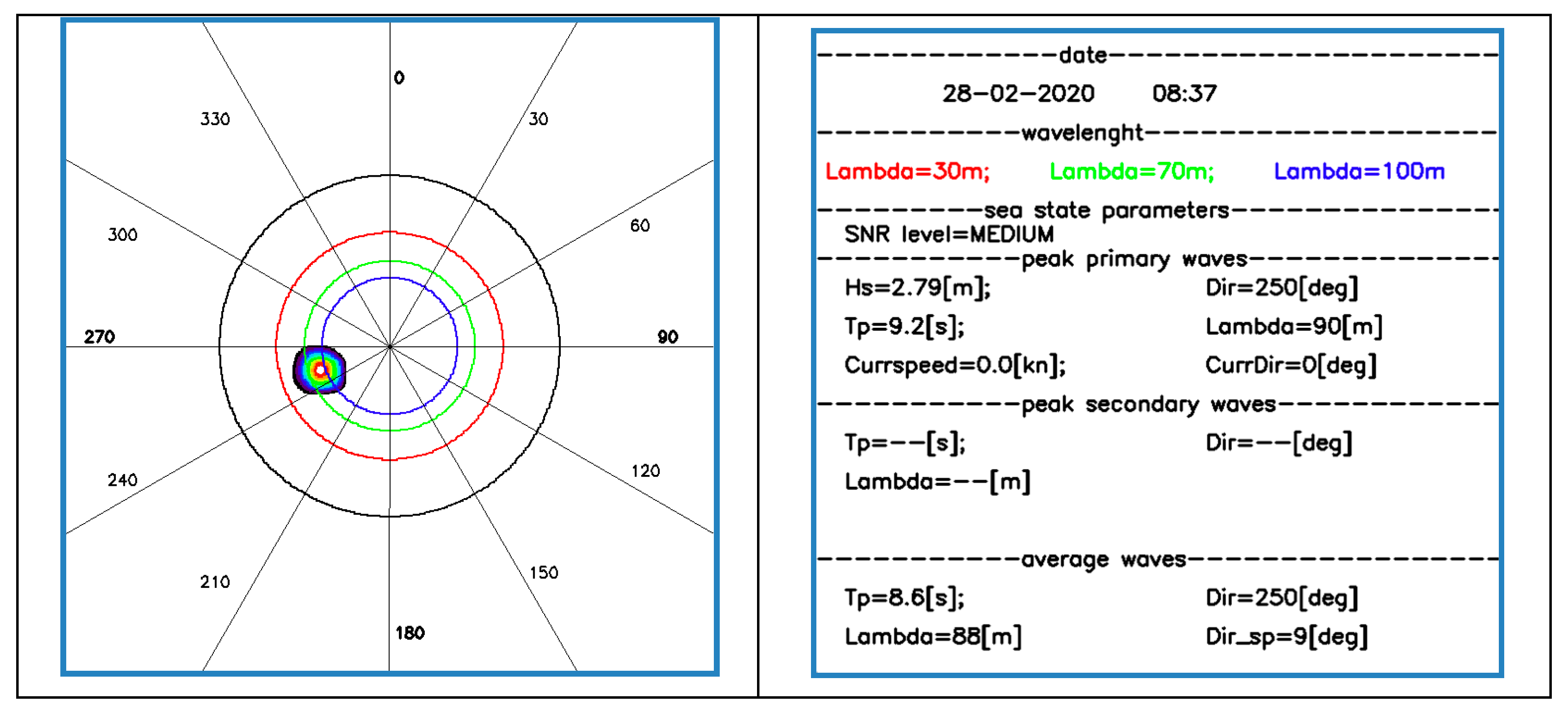
3.2. Sea State Parameters Measurements
3.3. Echosounder Survey
3.4. Hydrometer Measurements
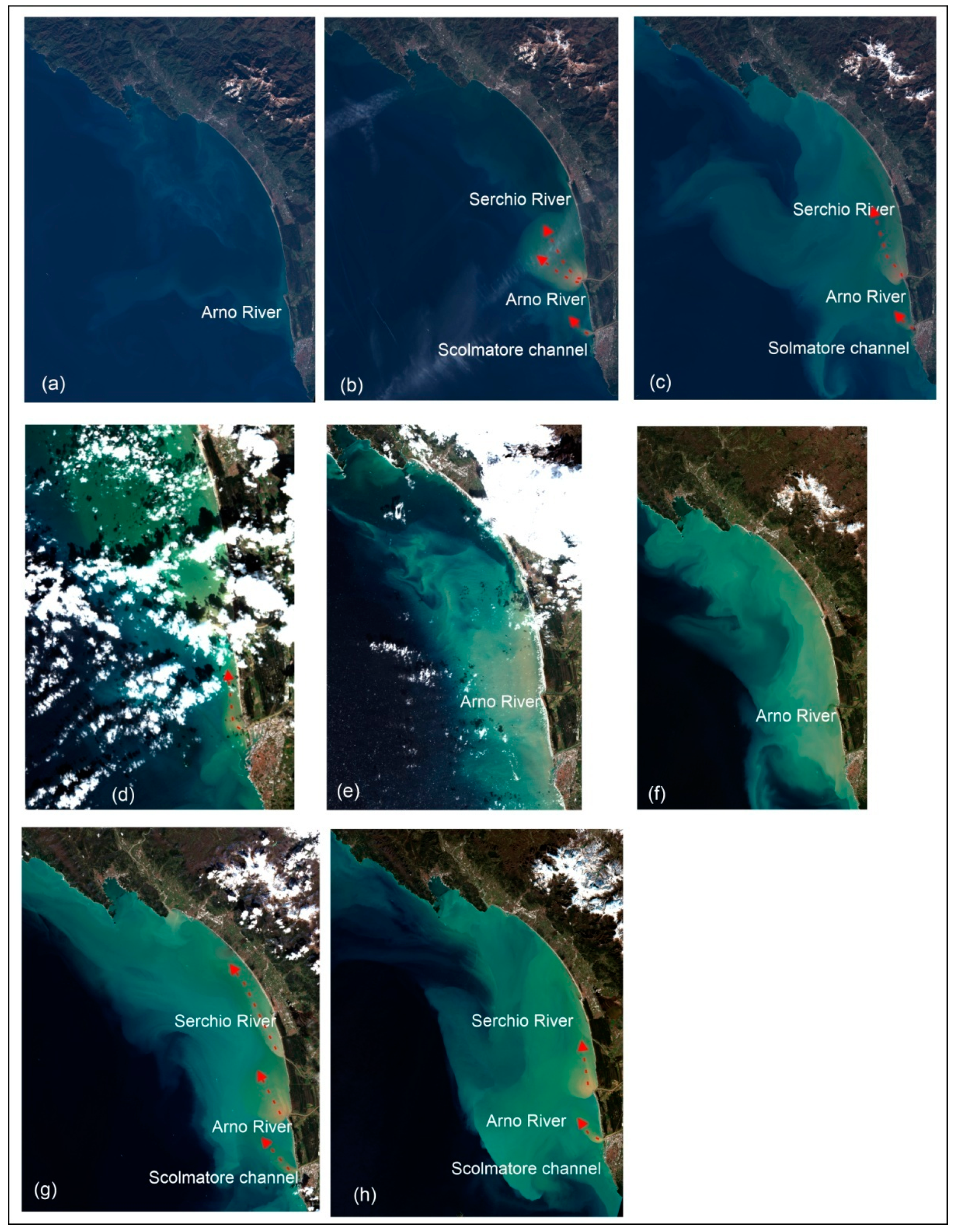
3.5. Satellite Images
4. Data Analysis
5. Discussion and Conclusions
Author Contributions
Funding
Data Availability Statement
Acknowledgments
Conflicts of Interest
References
- Masselink, G.; Russell, P. Impacts of climate change on coastal erosion. MCCIP Sci. Rev. 2013, 2013, 71–86. [Google Scholar]
- Coelho, C.; Silva, R.; Veloso-Gomes, F.; Taveira-Pinto, F. Potential effects of climate change on northwest Portuguese coastal zones. ICES J. Mar. Sci. 2009, 66, 1497–1507. [Google Scholar] [CrossRef] [Green Version]
- Pranzini, E.; Rosas, V. Pocket beach response to high magnitude—Low frequency floods (Elba Island, Italy). J. Coast. Res. 2007, 50, 969–977. [Google Scholar]
- Violante, C.; Biscarini, C.; Esposito, E.; Molisso, F.; Porfido, S.; Sacchi, M. The consequences of hydrological events on steep coastal watersheds: The Costa d’Amalfi, eastern Tyrrhenian Sea. In Proceedings of the Role of Hydrology in Water Resources Management Conference, Capri, Italy, 13–16 October 2008; IAHS Publ.: Foz do Iguaçu, Brazil, 2008; p. 327. [Google Scholar]
- Alberico, I.; Casalbore, D.; Pelosi, N.; Tonielli, R.; Calidonna, C.; Dominici, R.; De Rosa, R. Remote sensing and field survey data integration to investigate on the evolution of the coastal area. The case study of BagnaraCalabra (Southern Italy). Remote Sens. 2022, 14, 2459. [Google Scholar] [CrossRef]
- Alberico, I.; Iavarone, R.; Angrisani, A.C.; Castiello, A.; Incarnato, R.; Barra, R. The potential vulnerability indices as tools for natural risk reduction. The Volturno coastal plain case study. J. Coast. Conserv. 2017, 21, 743–758. [Google Scholar] [CrossRef]
- Sterzel, T.; Ludeke, M.K.B.; Walther, C.; Kok, M.T.; Sietz, D.; Lucas, P.L. Typology of coastal urban vulnerability under rapid urbanization. PLoS ONE 2020, 15, e0220936. [Google Scholar] [CrossRef] [Green Version]
- Wright, L.D.; Short, A.D. Morphodynamic variability of surf zones and beaches: A synthesis. Mar. Geol. 1984, 56, 93–118. [Google Scholar] [CrossRef]
- Cowell, P.J.; Thom, B.G. Morphodynamics of coastal evolution. In Coastal Evolution: Late Quaternary Shoreline Morphodynamics; Woodroffe, R.W.G., Carter, C.D., Eds.; Cambridge University Press: Cambridge, UK; New York, NY, USA, 1994; pp. 33–86. [Google Scholar]
- Hapke, C.J.; Himmelstoss, E.A.; Kratzmann, M.G.; List, J.H.; Thieler, E.R. National Assessment of Shoreline Change: Historical Shoreline Change Along the New England and Mid-Atlantic Coasts; U.S. Geological Survey: Reston, VI, USA, 2011; 57p. [Google Scholar]
- Li, X.; Zhou, Y.; Zhang, L.; Kuang, R. Shoreline change of Chongming Dongtan and response to river sediment load: A remote sensing assessment. J. Hydrol. 2014, 511, 432–442. [Google Scholar] [CrossRef]
- Mentaschi, L.; Vousdoukas, M.I.; Pekel, J.F.; Voukouvalas, E.; Feyen, L. Global long-term observations of coastal erosion and accretion. Sci. Rep. 2018, 8, 12876. [Google Scholar] [CrossRef] [Green Version]
- Li, D.; Tang, C.; Hou, X.; Zhang, H. Morphological changes in the Qinzhou Bay, Southwest China. J. Coast. Conserv. 2019, 23, 829–841. [Google Scholar] [CrossRef]
- Tătui, F.; Vespremeanu-Stroe, A.; Preoteasa, L. Alongshore Variations in Beach-Dune System Response to Major Storm Events on the Danube Delta Coast. J. Coas. Res. 2014, 70, 693–699. [Google Scholar] [CrossRef]
- Castelle, B.; Marieu, V.; Bujan, S.; Splinter, K.D.; Robinet, A.; Sénéchal, N.; Ferreira, S. Impact of the winter 2013–2014 series of severe Western Europe storms on a double-barred sandy coast: Beach and dune erosion and megacuspembayments. Geomorphology 2015, 238, 135–148. [Google Scholar] [CrossRef]
- Dissanayake, P.; Brown, J.; Karunarathna, H. Impacts of storm chronology on the morphological changes of the Formby beach and dune system. Nat. Hazards Earth Syst. Sci. 2015, 15, 1533–1543. [Google Scholar] [CrossRef] [Green Version]
- Johnson, J.M.; Moore, L.J.; Ells, K.; Murray, A.B.; Adams, P.N.; MacKenzie, R.A.; Jaeger, J.M. Recent shifts in coastline change and shoreline stabilization linked to storm climate change. Earth Surf. Process. Landf. 2014, 40, 585. [Google Scholar] [CrossRef]
- Senechal, N.; Coco, G.; Castelle, B.; Marieu, V. Storm impact on the seasonal shoreline dynamics of a meso- to macrotidal open sandy beach (Biscarrosse, France). Geomorphology 2015, 228, 448–461. [Google Scholar] [CrossRef]
- Ruiz de Alegria-Arzaburu, A.; Masselink, G. Storm response and beach rotation on a gravel beach, Slapton Sands. Mar. Geol. 2010, 278, 77–99. [Google Scholar] [CrossRef]
- Scott, D.; Charles Simpson, M.; Sim, R. The vulnerability of Caribbean coastal tourism to scenarios of climate change related sea level rise. J. Sustain. Tour. 2012, 20, 883–898. [Google Scholar] [CrossRef]
- Bird, C.O.; Bell, P.S.; Plater, A.J. Application of marine radar to monitoring seasonal and event-based changes in intertidal morphology. Geomorphology 2017, 285, 1–15. [Google Scholar] [CrossRef] [Green Version]
- Takewaka, S.; Tomoyuki, O. X-band radar observation of morphological changes due to flood events at the mouth of Tenryu River, Japan. Coast. Eng. J. 2018, 60, 387–399. [Google Scholar] [CrossRef]
- Rogowski, P.; de Paolo, T.; Terrill, E.; McNinch, J. X-band radar mapping of morphological changes at a dynamic coastal inlet. J. Geophys. Res. Earth Surf. 2018, 123, 3034–3054. [Google Scholar] [CrossRef]
- Rutten, J.; de Jong, S.M.; Ruessink, G. Accuracy of Nearshore Bathymetry Inverted From X-Band Radar and Optical Video Data. IEEE Trans. Geosci. Remote Sens. 2017, 55, 1106–1116. [Google Scholar] [CrossRef]
- Atkinson, J.; Esteves, L.S.; Williams, J.J.; Bell, P.S.; McCann, D.L. Nearshore monitoring with X-band radar: Maximizing utility in dynamic and complex environments. J. Geophys. Res. Oceans 2021, 126, e2020JC016841. [Google Scholar] [CrossRef]
- Holman, R.; Haller, M.C. Remote sensing of the nearshore. Annu. Rev. Mar. Sci. 2013, 5, 95–113. [Google Scholar] [CrossRef] [PubMed] [Green Version]
- Punzo, M.; Lanciano, C.; Tarallo, D.; Bianco, F.; Cavuoto, G.; De Rosa, R.; Di Fiore, V.; Cianflone, G.; Dominici, R.; Iavarone, M.; et al. Application of X-Band Wave Radar for Coastal Dynamic Analysis: Case Test of BagnaraCalabra (South Tyrrhenian Sea, Italy). J. Sens. 2016, 2016, 6236925. [Google Scholar] [CrossRef] [Green Version]
- Wallbridge, S.; Dolphin, T.; Taylor, C.J.L. X-band radar as a tool for monitoring natural coastal behaviour and potential development impacts. J. Oper. Oceanogr. 2018, 12, S199–S211. [Google Scholar] [CrossRef] [Green Version]
- Young, I.R.; Rosenthal, W.; Ziemer, F. A three-dimensional analysis of marine radar images for the determination of ocean wave directionality and surface currents. J. Geophys. Res. Oceans 1985, 90, 1049–1059. [Google Scholar] [CrossRef] [Green Version]
- Nieto-Borge, J.C.; RodrÍguez, G.R.; Hessner, K.; González, P.I. Inversion of marine radar images for surface wave analysis. J. Atmos. Ocean. Technol. 2004, 21, 1291–1300. [Google Scholar] [CrossRef]
- Nieto-Borge, J.C.; Hessner, K.; Jarabo-Amores, P.; de La Mata-Moya, D. Signal-to-noise ratio analysis to estimate ocean wave heights from X-band marine radar image time series. IET Radar Sonar Navig. 2008, 2, 35–41. [Google Scholar] [CrossRef] [Green Version]
- Senet, C.M.; Seemann, J.; Ziemer, F. The near-surface current velocity determined from image sequences of the sea surface. IEEE Trans. Geosci. Remote Sens. 2001, 39, 492–505. [Google Scholar] [CrossRef]
- Senet, C.M.; Seemann, J.; Flampouris, S.; Ziemer, F. Determination of bathymetric and current maps by the method DiSC based on the analysis of nautical X-band radar image sequences of the sea surface. IEEE Trans. Geosci. Remote Sens. 2008, 46, 2267–2279. [Google Scholar] [CrossRef]
- Hessner, K.; Nieto-Borge, J.C.; Bell, P.S. Nautical radar measurements in Europe: Applications of WaMoS II as a sensor for sea state, current and bathymetry. In Remote Sensing of the European Seas; Barale, V., Gade, M., Eds.; Springer: Dordrecht, The Netherlands, 2008; pp. 435–446. [Google Scholar] [CrossRef] [Green Version]
- Hessner, K.; Reichert, K.; Borge, J.C.N.; Stevens, C.L.; Smith, M.J. High-resolution X-band radar measurements of currents, bathymetry and sea state in highly inhomogeneous coastal areas. Ocean Dyn. 2014, 64, 989–998. [Google Scholar] [CrossRef]
- Ludeno, G.; Reale, F.; Dentale, F.; Pugliese Carratelli, E.; Natale, A.; Soldovieri, F.; Serafino, F. An X-Band Radar System for Bathymetry and Wave Field Analysis in a Harbour Area. Sensors 2015, 15, 1691–1707. [Google Scholar] [CrossRef] [PubMed] [Green Version]
- Serafino, F.; Ludeno, G.; Flampouris, S.; Soldovieri, F. Analysis of nautical X-band radar images for the generation of bathymetric map by the NSP method. In Proceedings of the Geoscience and Remote Sensing Symposium (IGARSS), Munich, Germany, 22–27 July 2012; pp. 2829–2832. [Google Scholar] [CrossRef]
- Bell, P.S. Shallow water bathymetry derived from an analysis of X-band marine radar images of waves. Coast. Eng. 1999, 37, 513–527. [Google Scholar] [CrossRef]
- Bell, P.S. Mapping shallow water coastal areas using a standard marine X-Band radar. In Proceedings of the Hydro8, Liverpool, UK, 4–6 November 2008; pp. 1–9. [Google Scholar]
- Bell, P.S.; Williams, J.J.; Clark, S.; Morris, B.D.; Vila-Concej, A. Nested radar systems for remote coastal observations. J. Coast. Res. 2006, 39, 483–487. [Google Scholar]
- Flampouris, S.; Seemann, J.; Ziemer, F. Sharing our experience using wave theories inversion for the determination of the local depth. In Proceedings of the OCEANS 2009—Europe Conference, Bremen, Germany, 11–14 May 2009; pp. 1–7. [Google Scholar] [CrossRef]
- Bell, P.S.; Osler, J.C. Mapping bathymetry using X-band marine radar data recorded from a moving vessel. Ocean Dyn. 2011, 61, 2141–2156. [Google Scholar] [CrossRef]
- Cavazza, S. Regionalizzazione geomorfologica del trasporto solido in sospensione dei corsi d’acqua tra il Magra e l’Ombrone. Atti Della Soc. Toscana Di Sci. Nat. Mem. Ser. A 1984, 91, 119–132. [Google Scholar]
- Gandolfi, G.; Paganelli, L. Il litorale pisano versiliese (area campione Alto Tirreno) composizione provenienza e dispersione delle sabbie. Boll. Soc. Geol. It. 1975, 94, 1273–1295. [Google Scholar]
- Bertoni, D.; Mencaroni, M. Four different coastal settings within the northern tuscany littoral cell: How did we get here? Atti Soc. Tosc. Sci. Nat. Ser. A 2018, 125, 55–68. [Google Scholar] [CrossRef]
- Piccardi, M.; Pranzini, E. Carte a piccola, grande e grandissima scala negli studi sull’evoluzione del litorale. Cosa è successo a Bocca d’Arno tra il XVI e il XIX secolo? L’Universo 2014, 5, 760–790. [Google Scholar]
- Linoli, A. Integrated Land and Water Resources Management. In Proceedings of the Special Session on History, Schriften der DWhG, Sonderband 2, Siegburg, Germany, 16 May 2005; ISBN 3-8334-2463-X. [Google Scholar]
- Pranzini, E. Updrift river mouth migration on cuspate deltas: Two examples from the coast of Tuscany (Italy). Geomorphology 2001, 38, 125–132. [Google Scholar] [CrossRef]
- Pranzini, E. Airborne LIDAR survey applied to the analysis of the historical evolution of the Arno River delta (Italy). J. Coast. Res. 2007, 50, 400–409. [Google Scholar]
- Borghi, L. Apporto Allo Studio Sulle Cause di Variazione del Litorale Pisano. Rass. Period. Cult. E Di Inf. 1970, 1–2, 11–12. [Google Scholar]
- Rapetti, F.; Vittorini, S. Osservazioni sulle variazioni dell’ala destra del Delta dell’Arno. Atti Soc. Tosc. Sci. Nat. Mem. Ser. A 1974, 81, 25–88. [Google Scholar]
- Bowman, D.; Pranzini, E. Reversed response within a segmented detached breakwater—The Gombo case, Tuscany coast, Italy. Coast. Eng. 2003, 49, 263–274. [Google Scholar] [CrossRef]
- Ciampalini, A.; Consoloni, I.; Salvatici, T.; Di Traglia, F.; Fidolini, F.; Sarti, G.; Moretti, S. Characterization of coastal environment by means of hyper-and multispectral techniques. Appl. Geogr. 2015, 57, 120–132. [Google Scholar] [CrossRef]
- Bini, M.; Casarosa, N.; Luppichini, M. Exploring the Relationship between River Discharge and Coastal Erosion: An Integrated Approach Applied to the Pisa Coastal Plain (Italy). Remote Sens. 2021, 13, 226. [Google Scholar] [CrossRef]
- Casarosa, N. Studio dell’evoluzione del litorale pisano tramite rilievi con GPS differenziale. Studi Costieri 2016, 23, 3–20. [Google Scholar]
- Sighieri, E. Le piene dell’Arno: Bonifiche. In Arti Grafiche; Mariotti, P., Ed.; Arti Grafiche Boccia: Salerno, SA, Italy, 1934; pp. 1–96. [Google Scholar]
- Cencetti, C.; Tacconi, P. The Fluvial Dynamics of the Arno River. G. Di Geol. Appl. 2005, 1, 193–202. [Google Scholar]
- Nardi, R. L’Arno e le Sue Acque: Contributo Conoscitivo per L’elaborazione del Piano di Bacino; Quaderno n. 1; Autorità di Bacino del fiume Arno: Firenze, Italy, 1993. [Google Scholar]
- Cipriani, L.E.; Ferri, S.; Iannotta, P.; Paolieri, F.; Pranzini, E. Morfologia e dinamica dei sedimenti del litorale della Toscana settentrionale. Studi Costieri 2001, 4, 119–156. [Google Scholar]
- Rapetti, F.; Vittorini, S. Osservazioni sul clima del litorale pisano. Riv. Geogr. It. 1978, 85, 1–26. [Google Scholar]
- Antonioli, F.; Lo Presti, V.; Rovere, A.; Ferranti, L.; Anzidei, M.; Furlani, S.; Mastronuzzi, G.; Orru, P.E.; Scicchitano, G.; Sannino, G.; et al. Analysis of tidal notches in the Mediterranean Sea. Quat. Sci. Rev. 2015, 119, 66–84. [Google Scholar] [CrossRef]
- Reichert, K.; Hessner, K.; Nieto-Borge, J.C.; Dittmer, J. WaMoS II: A radar based wave and current monitoring system. In Proceedings of the Ninth International Offshore and Polar Engineering Conference, Brest, France, 30 May−4 June 1999; p. 246. [Google Scholar]
- Nieto-Borge, J.C.; GuedesSoares, C. Analysis of directional wave fields using X-band navigation radar. Coast. Eng. 2000, 40, 375–391. [Google Scholar] [CrossRef]
- Ludeno, G.; Reale, F.; Raffa, F.; Dentale, F.; Soldovieri, F.; Pugliese Carratelli, E.; Serafino, F. Integration between X-Band Radar and Buoy Sea State Monitoring. J. Coast. Res. 2018, 34, 1358–1366. [Google Scholar] [CrossRef]
- Serafino, F.; Lugni, C.; Soldovieri, F. A Novel Strategy for the Surface Current Determination from Marine X-Band Radar data. IEEE Geosci. Remote Sens. Lett. 2010, 7, 231–235. [Google Scholar] [CrossRef]
- Ludeno, G.; Flampouris, S.; Lugni, C.; Soldovieri, F.; Serafino, F. A Novel Approach Based on Marine Radar Data Analysis for High-Resolution Bathymetry Map Generation. IEEE Geosci. Remote Sens. Lett. 2014, 11, 234–238. [Google Scholar] [CrossRef]
- Serafino, F.; Lugni, C.; Ludeno, G.; Arturi, D.; Uttieri, M.; Buonocore, B.; Zambianchi, E.; Budillon, G.; Soldovieri, F. REMOCEAN: A Flexible X-Band Radar System for Sea-State Monitoring and Surface Current Estimation. IEEE Geosci. Remote Sens. Lett. 2012, 9, 822–826. [Google Scholar] [CrossRef]
- Osadchiev, A.; Sedakov, R. Spreading dynamics of small river plumes off the northeastern coast of the Black Sea observed by Landsat 8 and Sentinel-2. Remote Sens. Environ. 2019, 221, 522–533. [Google Scholar] [CrossRef]


| Date | Hs (m) | Flow Rate (mc/s) | Note |
|---|---|---|---|
| 8 December 2016 | - | - | - |
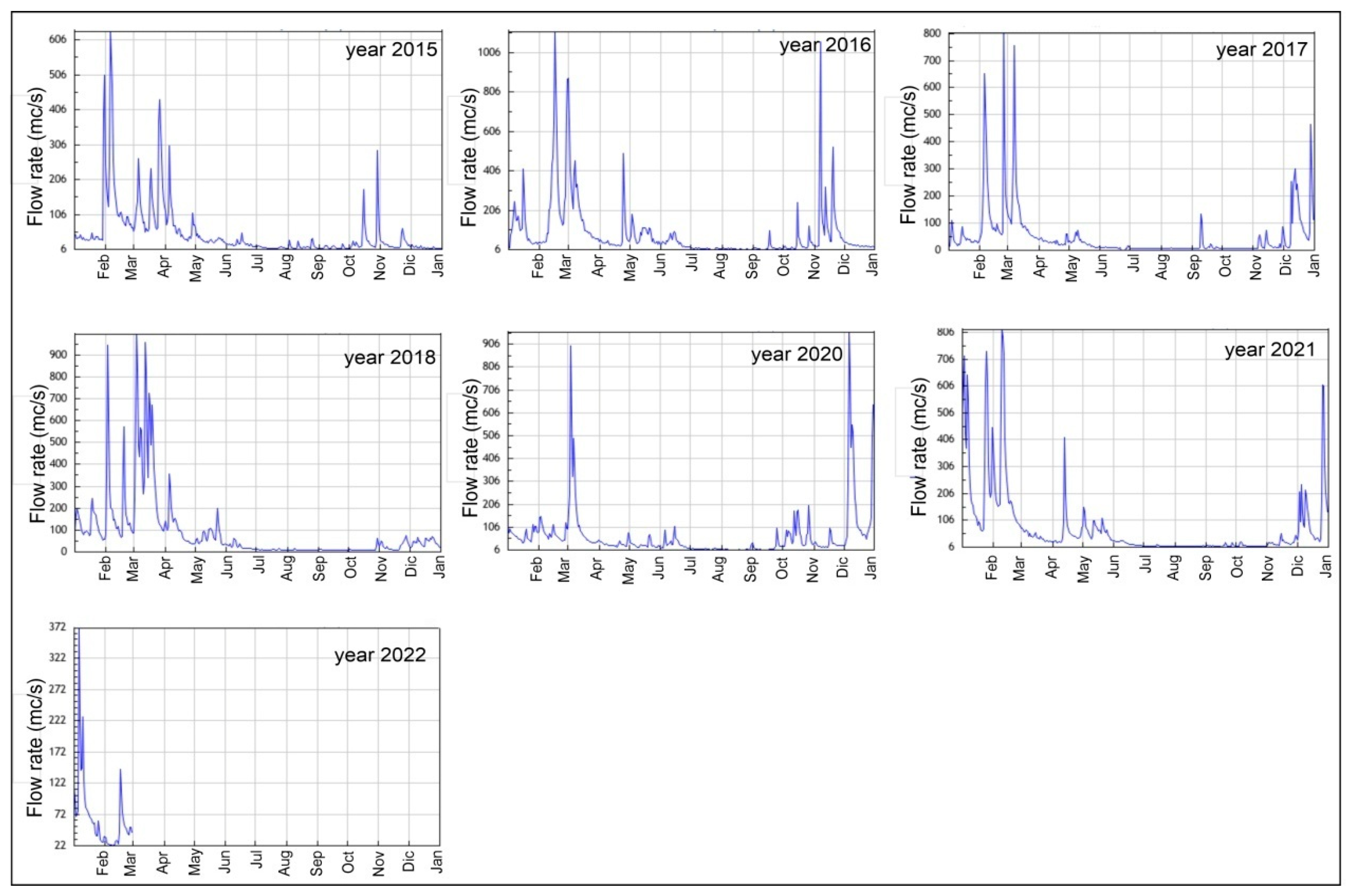
| 26 February 2017 | <1 | 421 | Hs = 2 m on 25 February; flow rate = 800 mc/s on 25 February |
| 8 March 2017 | 1 | 455 | Hs = 5 m from 5 to 7 March flow rate = 756 mc/s on 7 March |
| 8 March 2018 | 2.3 | 556 | flow rate = 567–993 mc/s from 7 to 3 March |
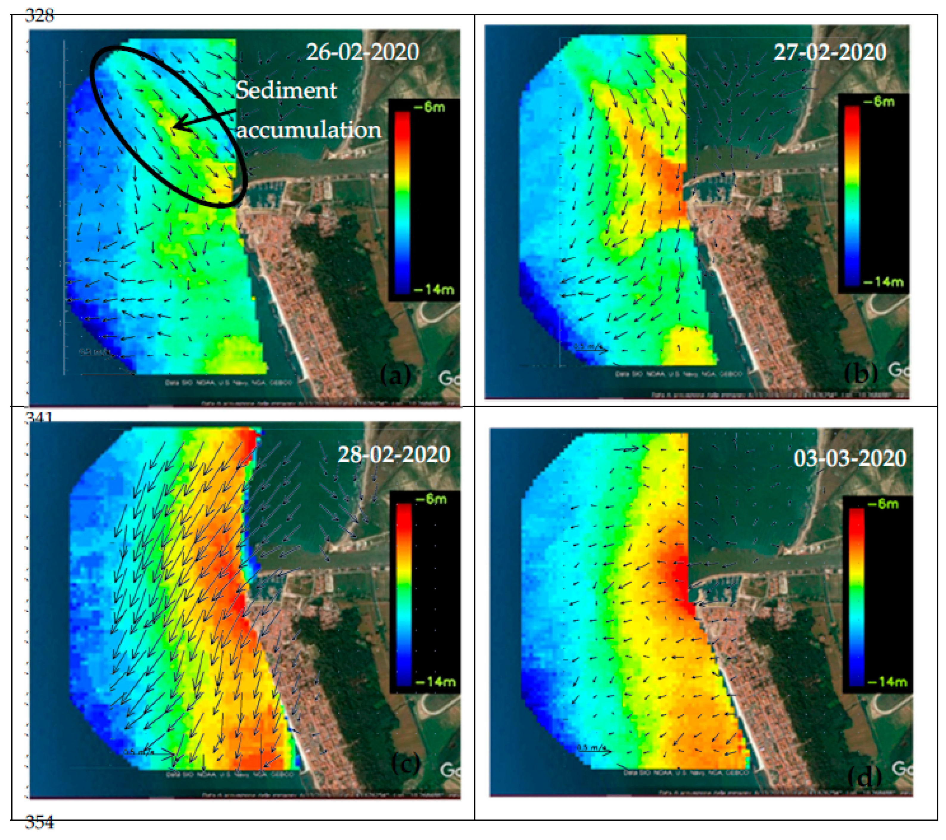
| 26 February 2020 | 5.5 | 48 | |
| 28 February 2020 | 4 | 124 | |
| 4 March 2020 | 3 | 592 | Hs = 3 m for several day before 4 March; flow rate= 897 mc/s on 3 March |
| 26 January 2021 | 1 | 622 | Hs = 5.3 m from 22 to 25 January |
Publisher’s Note: MDPI stays neutral with regard to jurisdictional claims in published maps and institutional affiliations. |
© 2022 by the authors. Licensee MDPI, Basel, Switzerland. This article is an open access article distributed under the terms and conditions of the Creative Commons Attribution (CC BY) license (https://creativecommons.org/licenses/by/4.0/).
Share and Cite
Raffa, F.; Alberico, I.; Serafino, F. X-Band Radar System to Detect Bathymetric Changes at River Mouths during Storm Surges: A Case Study of the Arno River. Sensors 2022, 22, 9415. https://doi.org/10.3390/s22239415
Raffa F, Alberico I, Serafino F. X-Band Radar System to Detect Bathymetric Changes at River Mouths during Storm Surges: A Case Study of the Arno River. Sensors. 2022; 22(23):9415. https://doi.org/10.3390/s22239415
Chicago/Turabian StyleRaffa, Francesco, Ines Alberico, and Francesco Serafino. 2022. "X-Band Radar System to Detect Bathymetric Changes at River Mouths during Storm Surges: A Case Study of the Arno River" Sensors 22, no. 23: 9415. https://doi.org/10.3390/s22239415