
Design of Cost-Efficient Optical Fronthaul for 5G/6G Networks: An Optimization Perspective


Abstract
:1. Introduction
- Formulation of an optimization framework based on ILP to obtain the optimal solution for 5G and beyond optical fronthaul design problems while minimizing the overall cost of the network.
- A proposal of two sub-optimal methods based on the K-means clustering and genetic algorithms, respectively, to overcome the ILP scalability issue.
- Assessment of the applicability of our proposed solutions by using them to optimize the deployment in two different scenarios (dense and sparse configurations).
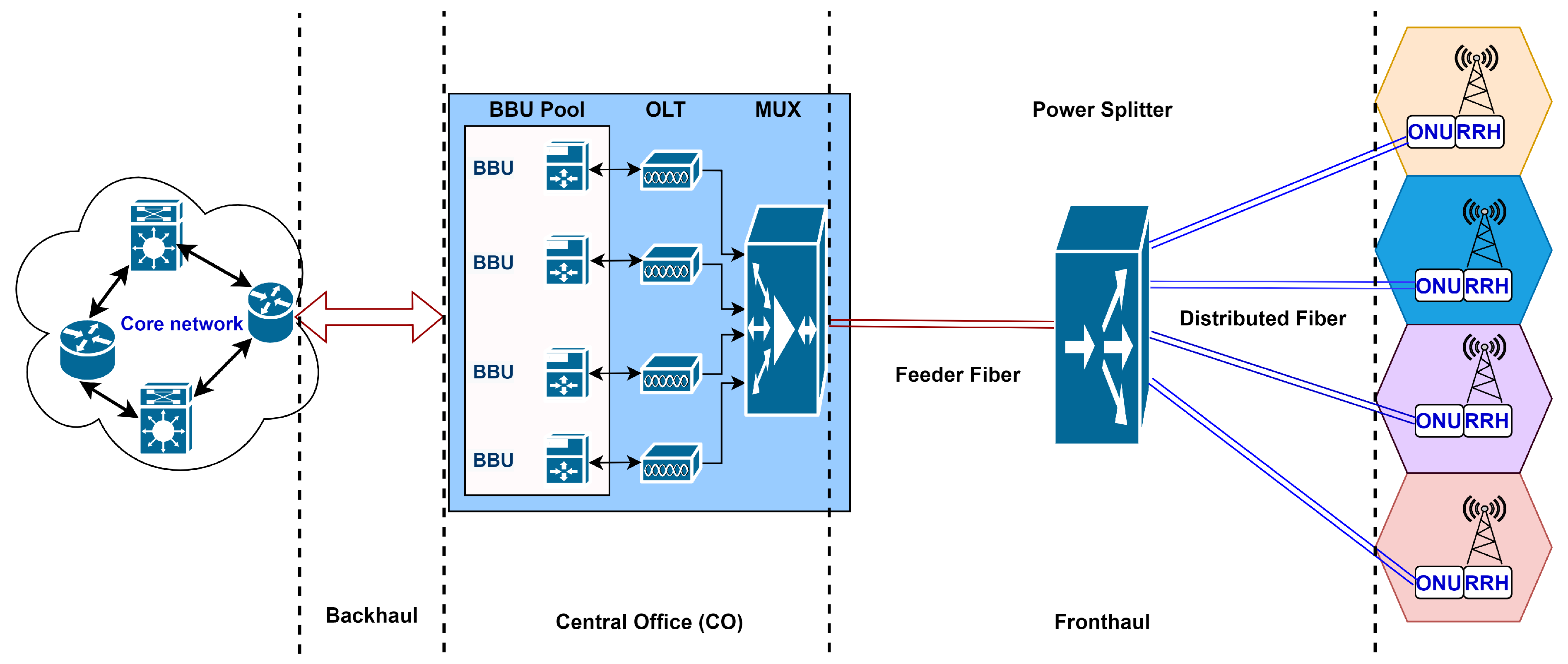
2. xRAN Architecture Developments and Fronthaul Enabling Technologies
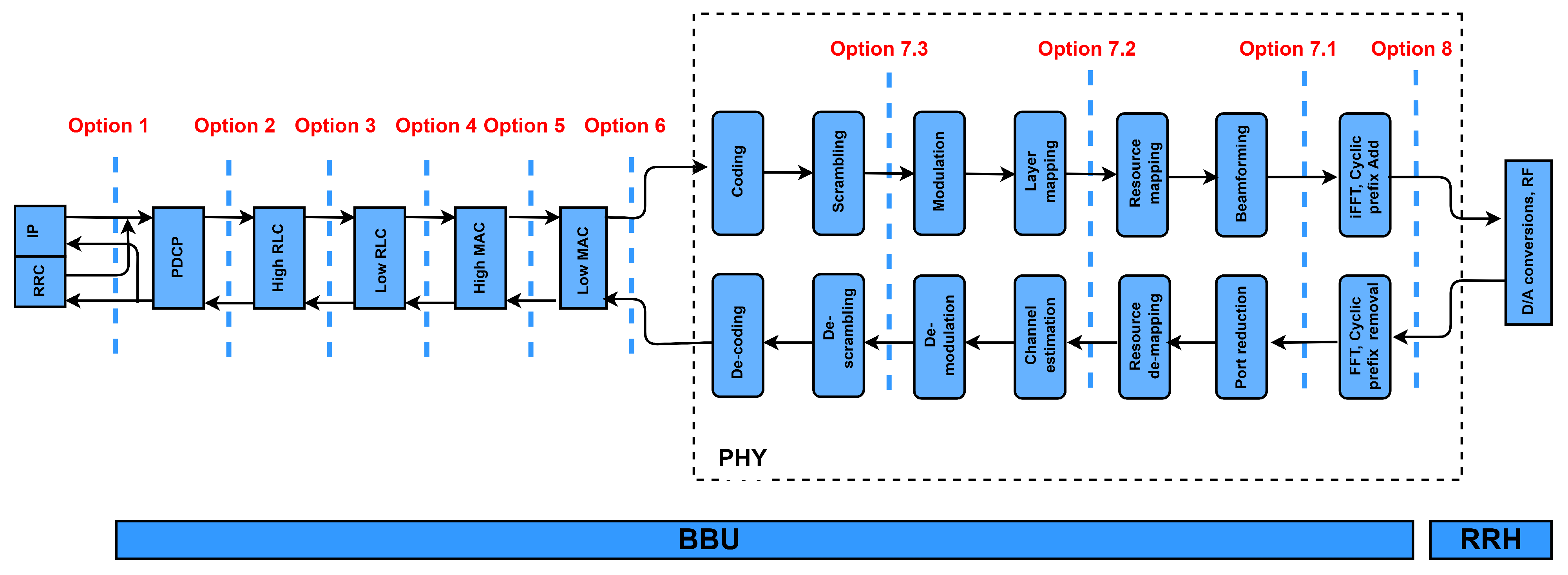
2.1. CRAN Architecture and Functional Splits
- Cost and footprint efficiency as it requires less hardware.
- Low energy consumption.
- Simple and flexible architecture.
- Resource and infrastructure sharing.
- Increased efficiency of network upgrades and enhancements.
- Ease of testing and maintenance.

2.2. Technologies Enabling 5G and beyond Fronthaul
3. Related Work
4. Problem Description
- Power splitter placement: Depending on the RRH location and splitter ratio capacity, we have to determine the best possible location to assign splitters to RRHs according to their maximum ratio capacity. The shortest distance and lowest delay are used to divide all RRHs into groups. This is a clustering problem since each set of RRHs is assigned to one splitter and is known to be NP-complete [47].
- BBU pool placement: According to the splitter locations, the optimal location for the BBU pool is near the center of the splitters group in order to keep the overall length of the link between the splitters and the BBU pool within the group to a minimum.
- Fronthaul deployment: To find the optimal fronthaul deployment over the network, all RRHs must be connected to the splitter based on the shortest path possible, and all splitters must be linked to the BBU pool according to the shortest distance.
- How to establish RRH groups that are all linked to one power splitter?
- How to find the optimal location for the BBU pool while resulting in the minimal cost?
- How to find the shortest path from the RRH to its splitter and from the splitter to the BBU pool?
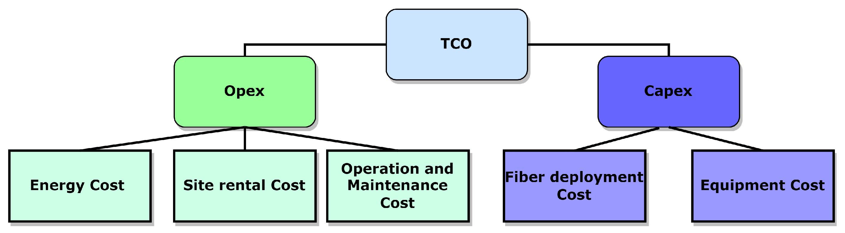
Cost Model
5. ILP Formulation and Heuristic Solutions
5.1. Network Data Sets and Input Parameters
5.2. Decision Variables
5.3. Objective Function
5.4. Constraints
- Topology constraints
- (a)
- The RRH can be connected to one power splitter only:
- (b)
- The number of RRHs that are connected to one splitter can not exceed the splitting ratio:
- (c)
- If there is an optical link from a splitter to an RRH, it should be installed at a viable splitter location:
- (d)
- If a splitter is used at a possible site, it must be connected to at least one RRH:
- (e)
- Each splitter can be served by only one BBU pool:
- (f)
- The number of BBU pools can not exceed the maximum number:
- (g)
- If an optical path exists between a BBU pool and a splitter, the splitter must be connected to at least one RRH:
- (h)
- The number of needed splitters should be calculated as follows:
- (i)
- The number of BBUs should be calculated as follows:
- (j)
- The number of OLTs and the number of AWGs in the network should be equal to the total number of splitters:
- Capacity constraints
- (a)
- The capacity referring to the downlink transmission must be equal to or less than the maximum downlink capacity of TWDM-PON:
- (b)
- The capacity referring to the uplink transmission must be equal to or less than the maximum uplink capacity of TWDM-PON:
- Distance constraints
- (a)
- The maximum length of the distribution fiber should not surpass the maximum specific length:
- (b)
- The distance between each RRH and its serving BBU pool must be less than the maximum distance allowed in PONs:
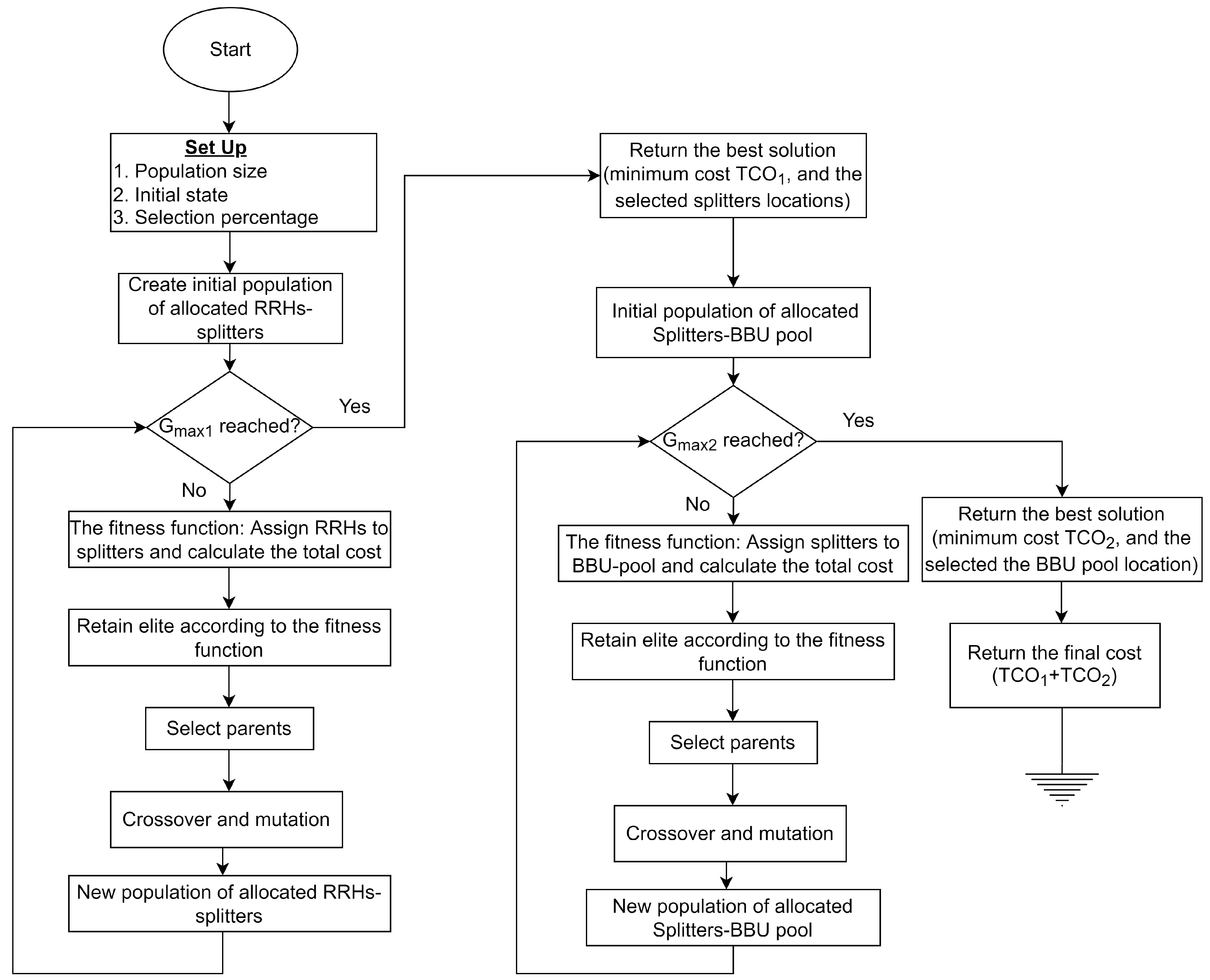
5.5. Heuristic Approach
5.5.1. K-means Clustering Algorithm
| Algorithm 1 Cost-effective optical fronthaul design algorithm based on K-means clustering. |
Input:B, P, N, , , , , , , , , , E, , , , , , , maximum number of replications Output: Optimal optical fronthaul deployment, optimal TCO
|
5.5.2. Genetic Algorithm
| Algorithm 2 Cost-effective optical fronthaul design based on the GA. |
Input:B, P, N,, , , , , , , , , E, , , , , maximum number of replications, population size (), maximum number of generations (), number of elites in each generation (), mutation rate (), , , ,. Output: Optimal optical fronthaul deployment, optimal TCO.
|
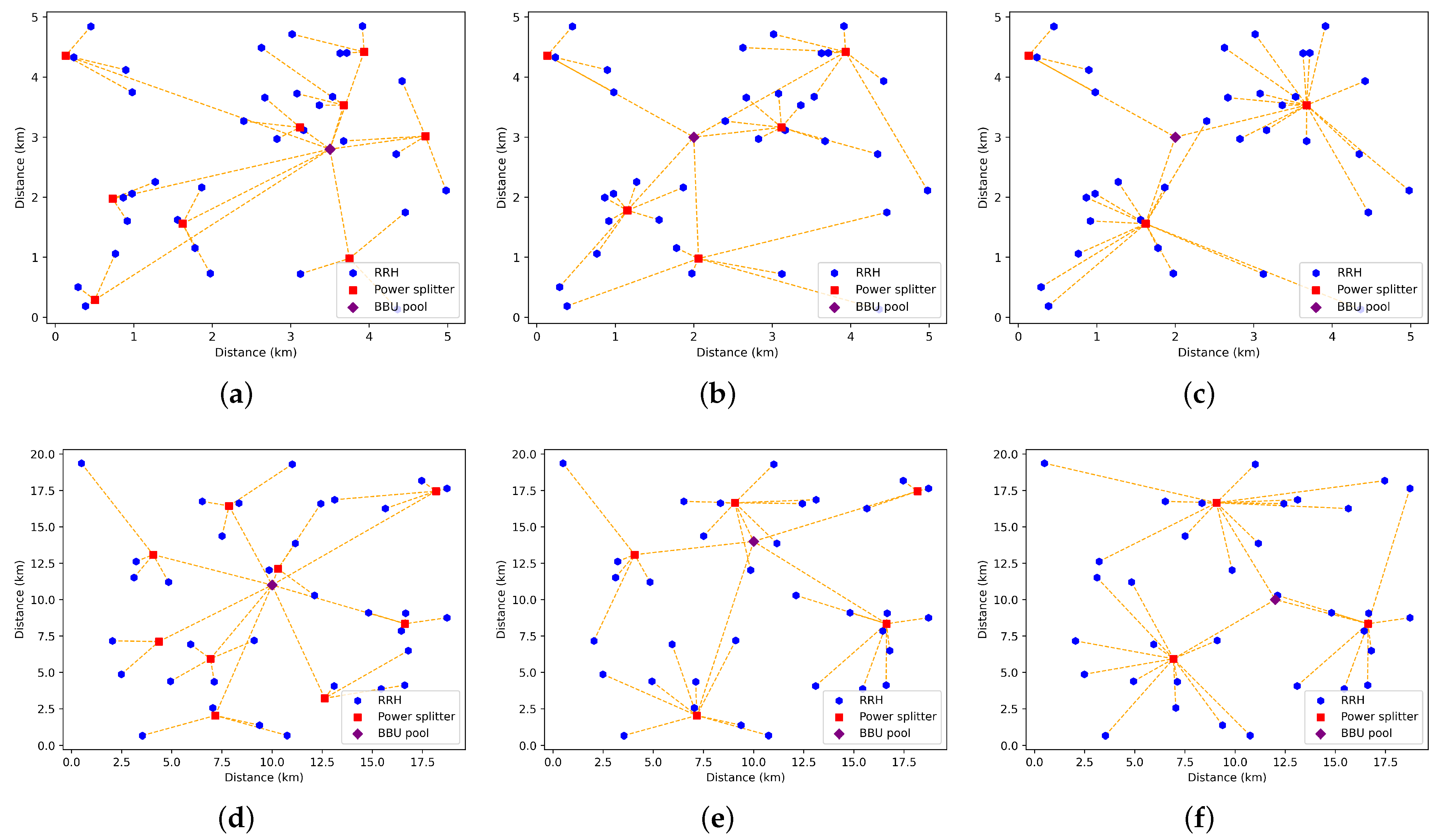
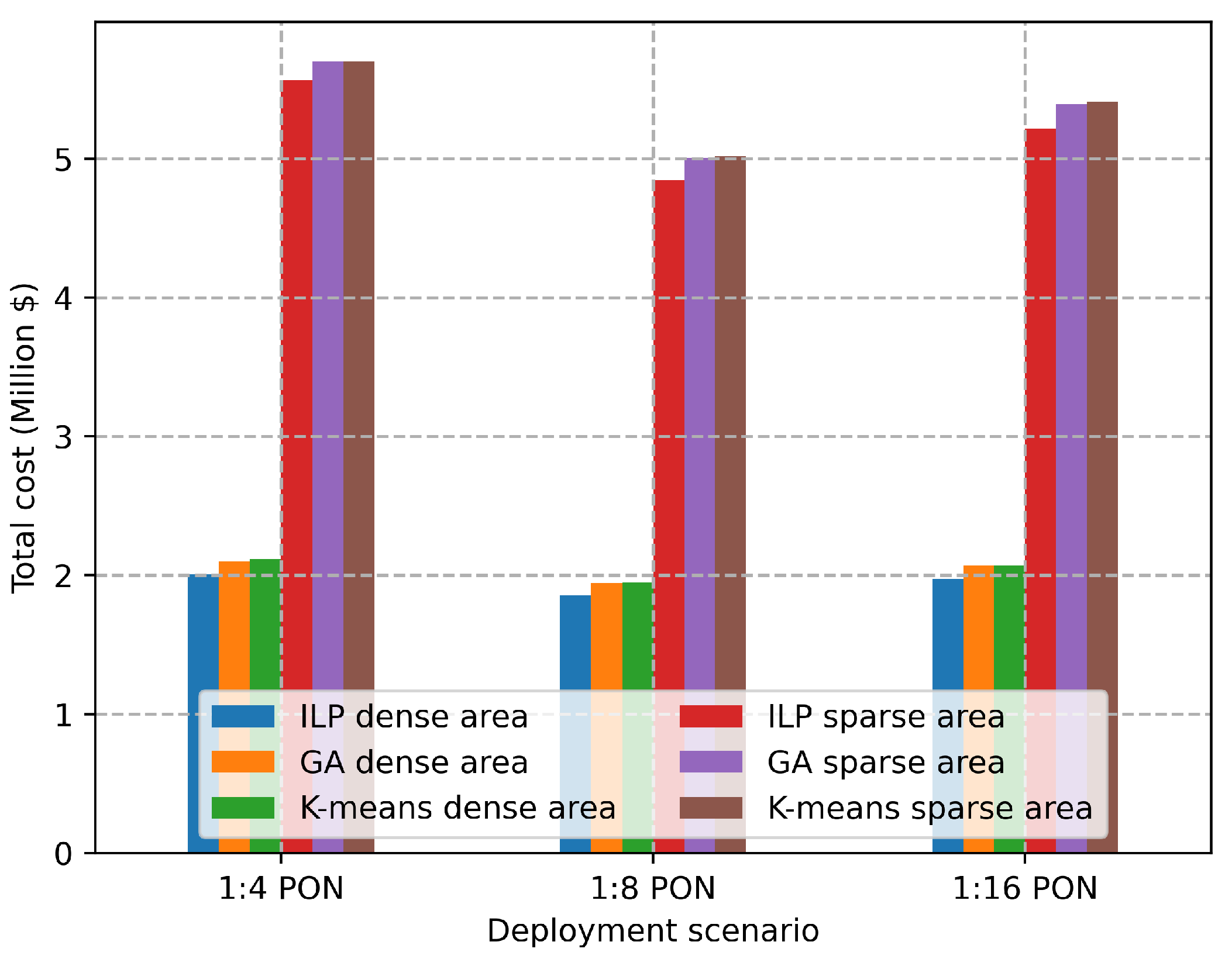
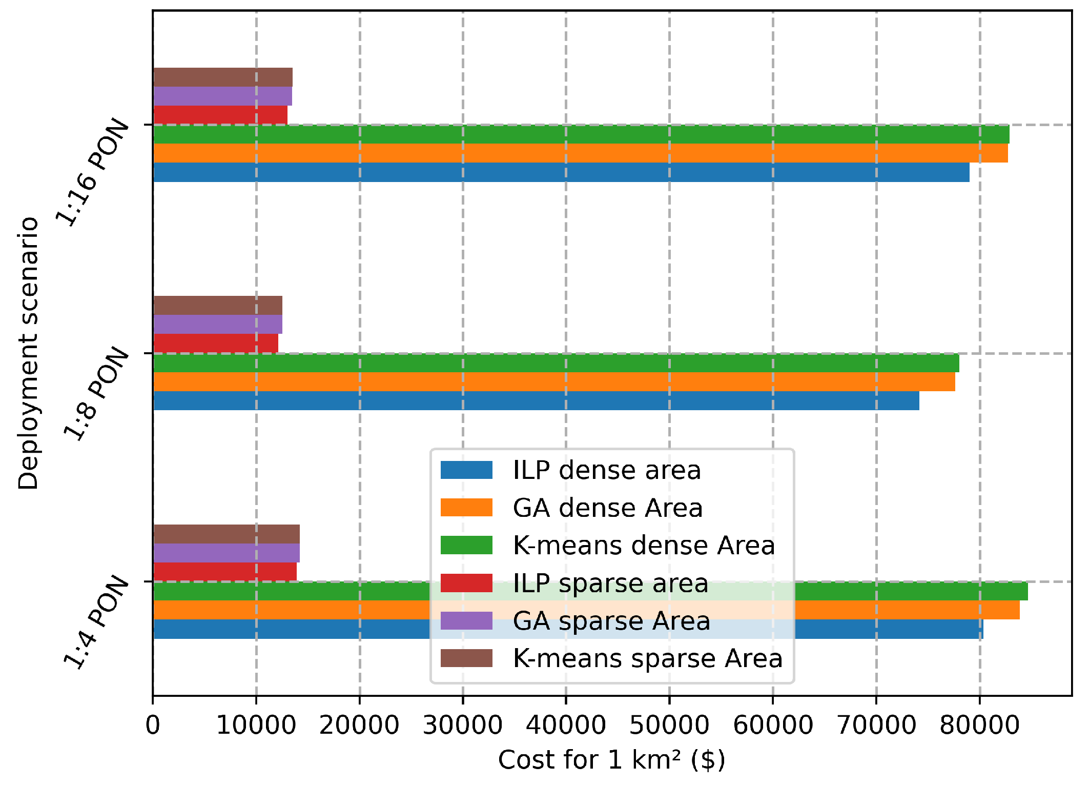
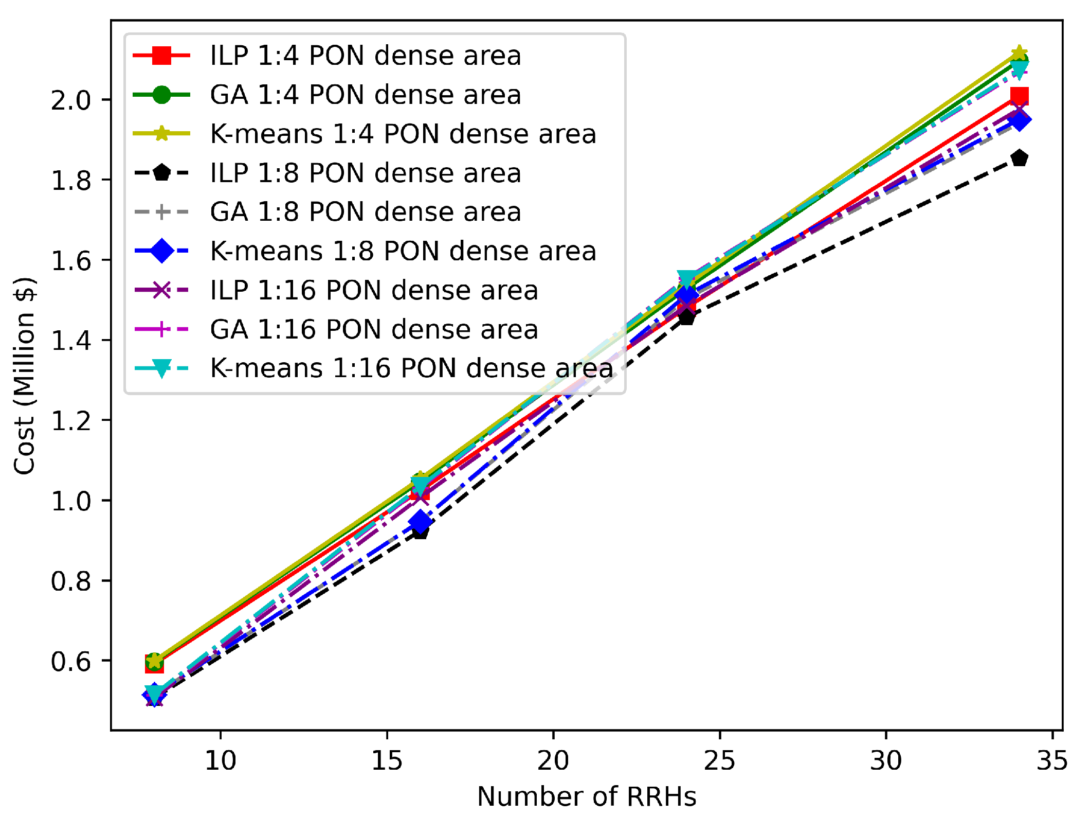
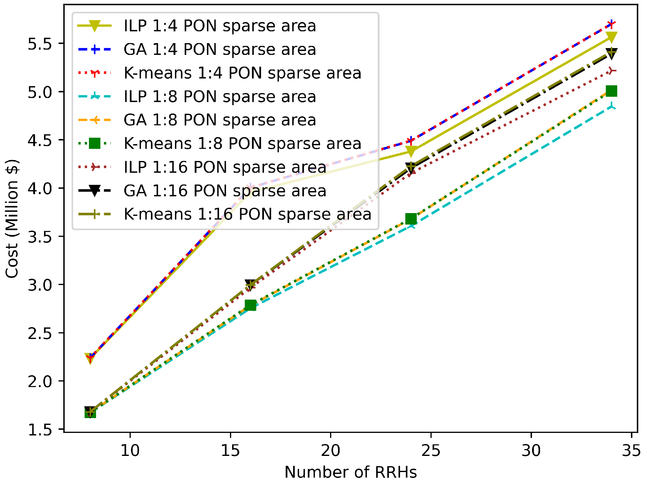
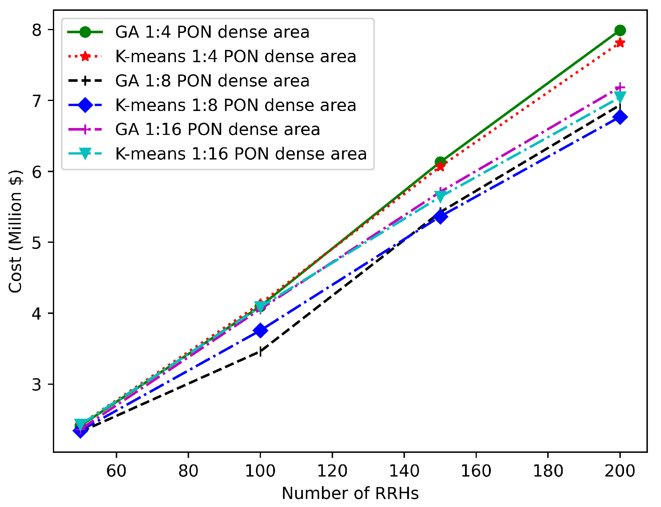
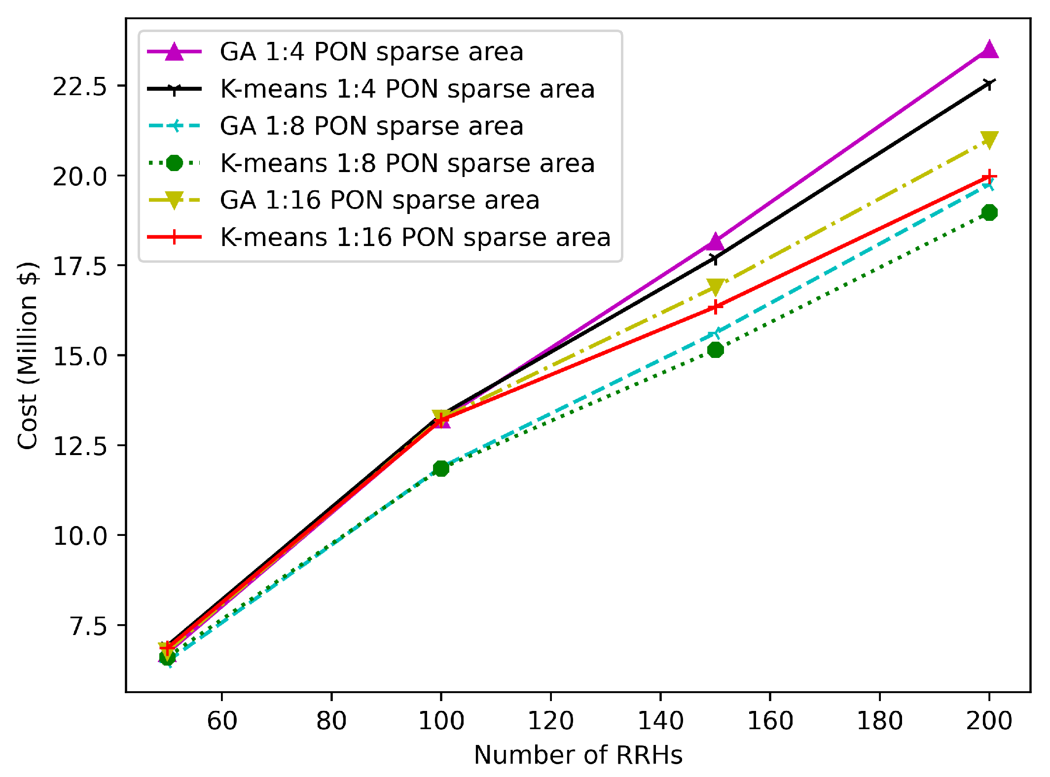
6. Case Study and Numerical Results
6.1. Simulation Setup
6.2. Results and Discussion
7. Conclusions
Author Contributions
Funding
Institutional Review Board Statement
Informed Consent Statement
Data Availability Statement
Acknowledgments
Conflicts of Interest
References
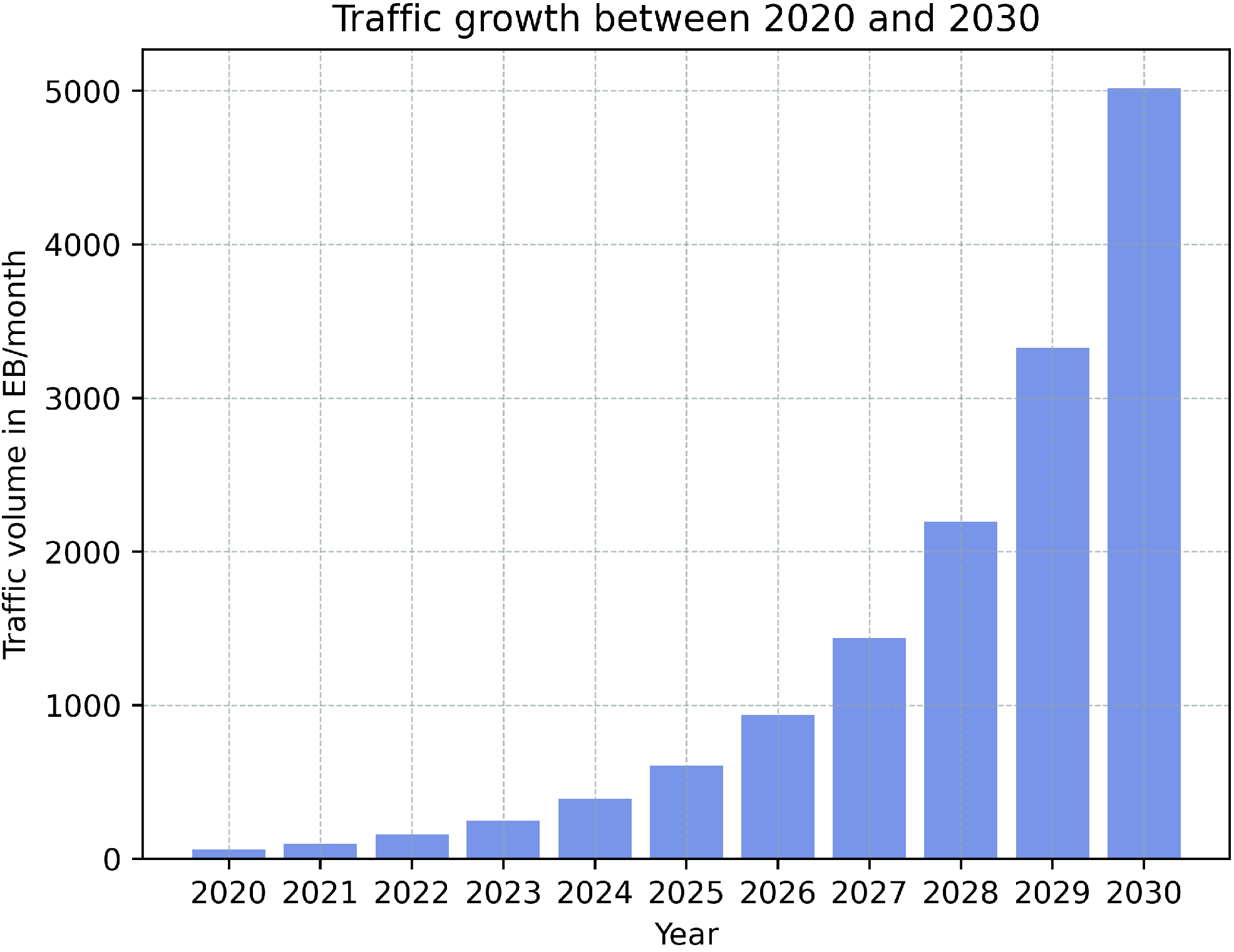
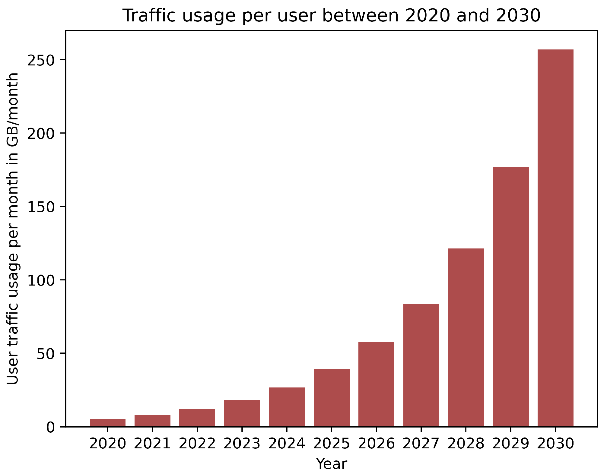
- ITU-R. IMT Traffic Estimates for the Years 2020 to 2030. ITU. Available online: www.itu.int/pub/R-REP-M.2370-2015 (accessed on 11 October 2022).
- Agiwal, M.; Roy, A.; Saxena, N. Next generation 5G wireless networks: A comprehensive survey. IEEE Commun. Surv. Tutor. 2016, 18, 1617–1655. [Google Scholar] [CrossRef]
- Jiang, W.; Han, B.; Habibi, M.A.; Schotten, H.D. The road towards 6G: A comprehensive survey. IEEE Open J. Commun. Soc. 2021, 2, 334–366. [Google Scholar] [CrossRef]
- Khan, W.U.; Mahmood, A.; Bozorgchenani, A.; Jamshed, M.A.; Ranjha, A.; Lagunas, E.; Pervaiz, H.; Chatzinotas, S.; Ottersten, B.; Popovski, P. Opportunities for Intelligent Reflecting Surfaces in 6G-Empowered V2X Communications. arXiv 2022, arXiv:2210.00494. [Google Scholar]
- Hakeem, S.A.A.; Hussein, H.H.; Kim, H. Vision and research directions of 6G technologies and applications. J. King Saud Univ.-Comput. Inf. Sci. 2022, 34, 2419–2442. [Google Scholar]
- Khan, W.U.; Javed, M.A.; Zeadally, S.; Lagunas, E.; Chatzinotas, S. Intelligent and Secure Radio Environments for 6G Vehicular Aided HetNets: Key Opportunities and Challenges. arXiv 2022, arXiv:2210.02172. [Google Scholar]
- Alimi, I.A.; Teixeira, A.L.; Monteiro, P.P. Toward an efficient C-RAN optical fronthaul for the future networks: A tutorial on technologies, requirements, challenges, and solutions. IEEE Commun. Surv. Tutor. 2017, 20, 708–769. [Google Scholar] [CrossRef]
- Katti, R.; Prince, S. A survey on role of photonic technologies in 5G communication systems. Photonic Netw. Commun. 2019, 38, 185–205. [Google Scholar] [CrossRef]
- Lagkas, T.; Klonidis, D.; Sarigiannidis, P.; Tomkos, I. Optimized Joint Allocation of Radio, Optical, and MEC Resources for the 5G and Beyond Fronthaul. IEEE Trans. Netw. Serv. Manag. 2021, 18, 4639–4653. [Google Scholar] [CrossRef]
- Peng, M.; Li, Y.; Jiang, J.; Li, J.; Wang, C. Heterogeneous cloud radio access networks: A new perspective for enhancing spectral and energy efficiencies. IEEE Wirel. Commun. 2014, 21, 126–135. [Google Scholar] [CrossRef] [Green Version]
- Peng, M.; Yan, S.; Zhang, K.; Wang, C. Fog-computing-based radio access networks: Issues and challenges. IEEE Netw. 2016, 30, 46–53. [Google Scholar] [CrossRef] [Green Version]
- Singh, S.K.; Singh, R.; Kumbhani, B. The evolution of radio access network towards open-RAN: Challenges and opportunities. In Proceedings of the 2020 IEEE Wireless Communications and Networking Conference Workshops (WCNCW), Seoul, Republic of Korea, 6–9 April 2020; pp. 1–6. [Google Scholar]
- Transport Network Support of IMT-2020/5G—ITU Hub. ITU Hub. Available online: www.itu.int/hub/publication/t-tut-home-2018 (accessed on 4 October 2022).
- Wang, X.; Cavdar, C.; Wang, L.; Tornatore, M.; Zhao, Y.; Chung, H.S.; Lee, H.H.; Park, S.; Mukherjee, B. Joint allocation of radio and optical resources in virtualized cloud RAN with CoMP. In Proceedings of the 2016 IEEE Global Communications Conference (GLOBECOM), Washington, DC, USA, 4–8 December 2016; pp. 1–6. [Google Scholar]
- 3GPP TR 38.801. Study on New Radio Access Technology: Radio Access Architecture and Interfaces. StandICT.eu. 19 August 2019. Available online: 2020.standict.eu/standards-watch/study-new-radio-access-technology-radio-access-architecture-and-interfaces (accessed on 6 October 2022).
- Gomes, N.J.; Assimakopoulos, P. Optical fronthaul options for meeting 5G requirements. In Proceedings of the 2018 20th International Conference on Transparent Optical Networks (ICTON), Bucharest, Romania, 1–5 July 2018; pp. 1–4. [Google Scholar]
- Larsen, L.M.; Checko, A.; Christiansen, H.L. A survey of the functional splits proposed for 5G mobile crosshaul networks. IEEE Commun. Surv. Tutor. 2018, 21, 146–172. [Google Scholar] [CrossRef] [Green Version]
- Skubic, B.; Fiorani, M.; Tombaz, S.; Furuskär, A.; Mårtensson, J.; Monti, P. Optical transport solutions for 5G fixed wireless access. J. Opt. Commun. Netw. 2017, 9, D10–D18. [Google Scholar] [CrossRef]
- Ranaweera, C.; Monti, P.; Skubic, B.; Wong, E.; Furdek, M.; Wosinska, L.; Machuca, C.M.; Nirmalathas, A.; Lim, C. Optical transport network design for 5G fixed wireless access. J. Light. Technol. 2019, 37, 3893–3901. [Google Scholar] [CrossRef]
- Yaacoub, E.; Alouini, M.S. A key 6G challenge and opportunity—Connecting the base of the pyramid: A survey on rural connectivity. Proc. IEEE 2020, 108, 533–582. [Google Scholar] [CrossRef] [Green Version]
- Ladányi, Á.; Cinkler, T. Resilience–throughput–power trade-off in future 5G photonic networks. Photonic Netw. Commun. 2019, 37, 296–310. [Google Scholar] [CrossRef] [Green Version]
- Fayad, A.; Alqhazaly, Q.; Cinkler, T. Time and Wavelength Division Multiplexing Passive Optical Network comparative analysis: Modulation formats and channel spacings. Int. J. Electron. Commun. Eng. 2021, 15, 231–237. [Google Scholar]
- ITU-T G.989.3: 40-Gigabit-Capable Passive Optical Networks (NG-PON2): Transmission Convergence Layer Specification. 30 September 2021. Available online: www.itu.int/rec/T-REC-G.989.3-202105-I/en (accessed on 26 November 2022).
- Nakayama, Y.; Hisano, D. Wavelength and bandwidth allocation for mobile fronthaul in TWDM-PON. IEEE Trans. Commun. 2019, 67, 7642–7655. [Google Scholar] [CrossRef]
- Fayad, A.; Jha, M.; Cinkler, T.; Rak, J. Planning a Cost-Effective Delay-Constrained Passive Optical Network for 5G Fronthaul. In Proceedings of the 2022 International Conference on Optical Network Design and Modeling (ONDM), Warsaw, Poland, 16–19 May 2022; pp. 1–6. [Google Scholar]
- Mitcsenkov, A.; Paksy, G.; Cinkler, T. Geography-and infrastructure-aware topology design methodology for broadband access networks (FTTx). Photonic Netw. Commun. 2011, 21, 253–266. [Google Scholar] [CrossRef]
- Jaffer, S.S.; Hussain, A.; Qureshi, M.A.; Mirza, J.; Qureshi, K.K. A low cost PON-FSO based fronthaul solution for 5G CRAN architecture. Opt. Fiber Technol. 2021, 63, 102500. [Google Scholar] [CrossRef]
- Kalesnikau, I.; Pióro, M.; Rak, J.; Ivanov, H.; Fitzgerald, E.; Leitgeb, E. Enhancing Resilience of FSO Networks to Adverse Weather Conditions. IEEE Access 2021, 9, 123541–123565. [Google Scholar] [CrossRef]
- Fayad, A.; Cinkler, T. Cost-Effective Delay-Constrained Optical Fronthaul Design for 5G and Beyond. Infocommun. J. 2022, 14, 19–27. [Google Scholar] [CrossRef]
- Rony, R.I.; Lopez-Aguilera, E.; Garcia-Villegas, E. Cost Analysis of 5G Fronthaul Networks Through Functional Splits at the PHY Layer in a Capacity and Cost Limited Scenario. IEEE Access 2021, 9, 8733–8750. [Google Scholar] [CrossRef]
- TEAM, ETSI COMS. “ETSI—ETSI Publishes Report on 5G Wireless Backhaul/X-Haul.” ETSI—ETSI Publishes. Report on 5G Wireless Backhaul/X-Haul. Available online: www.etsi.org/committee?id=1465 (accessed on 11 November 2022).
- Hilt, A. Microwave hop-length and availability targets for the 5G mobile backhaul. In Proceedings of the 2019 42nd International Conference on Telecommunications and Signal Processing (TSP), Budapest, Hungary, 1–3 July 2019; pp. 187–190. [Google Scholar]
- Musumeci, F.; Bellanzon, C.; Carapellese, N.; Tornatore, M.; Pattavina, A.; Gosselin, S. Optimal BBU placement for 5G C-RAN deployment over WDM aggregation networks. J. Light. Technol. 2016, 34, 1963–1970. [Google Scholar] [CrossRef]
- Chen, H.; Li, Y.; Bose, S.K.; Shao, W.; Xiang, L.; Ma, Y.; Shen, G. Cost-minimized design for TWDM-PON-based 5G mobile backhaul networks. J. Opt. Commun. Netw. 2016, 8, B1–B11. [Google Scholar] [CrossRef]
- Klinkowski, M. Planning of 5G C-RAN with optical fronthaul: A scalability analysis of an ILP model. In Proceedings of the 2018 20th International Conference on Transparent Optical Networks (ICTON), Bucharest, Romania, 1–5 July 2018; pp. 1–4. [Google Scholar]
- Ranaweera, C.; Nirmalathas, A.; Wong, E.; Lim, C.; Monti, P.; Furdek, M.; Wosinska, L.; Skubic, B.; Machuca, C.M. Rethinking of Optical Transport Network Design for 5G/6G Mobile Communication. IEEE Future Netw. 2021, 12. Available online: https://futurenetworks.ieee.org/tech-focus/april-2021/rethinking-ofoptical-transport-network-design-for-5g-6g-mobile-communication (accessed on 11 November 2022).
- Masoudi, M.; Lisi, S.S.; Cavdar, C. Cost-effective migration toward virtualized C-RAN with scalable fronthaul design. IEEE Syst. J. 2020, 14, 5100–5110. [Google Scholar] [CrossRef]
- Marotta, A.; Correia, L.M. Cost-effective joint optimisation of BBU placement and fronthaul deployment in brown-field scenarios. EURASIP J. Wirel. Commun. Netw. 2020, 2020, 1–26. [Google Scholar] [CrossRef]
- Ranaweera, C.; Lim, C.; Nirmalathas, A.; Jayasundara, C.; Wong, E. Cost-optimal placement and backhauling of small-cell networks. J. Light. Technol. 2015, 33, 3850–3857. [Google Scholar] [CrossRef]
- Ranaweera, C.; Resende, M.G.; Reichmann, K.; Iannone, P.; Henry, P.; Kim, B.J.; Magill, P.; Oikonomou, K.N.; Sinha, R.K.; Woodward, S. Design and optimization of fiber optic small-cell backhaul based on an existing fiber-to-the-node residential access network. IEEE Commun. Mag. 2013, 51, 62–69. [Google Scholar] [CrossRef]
- Kolydakis, N.; Tomkos, I. A techno-economic evaluation of different strategies for front-/back-hauling of mobile traffic: Wireless versus fiber based solutions. In Proceedings of the 2014 16th International Conference on Transparent Optical Networks (ICTON), Graz, Austria, 6–10 July 2014; pp. 1–4. [Google Scholar]
- Jarray, A.; Jaumard, B.; Houle, A.C. Reducing the CAPEX and OPEX costs of optical backbone networks. In Proceedings of the 2010 IEEE International Conference on Communications, Cape Town, South Africa, 23–27 May 2010; pp. 1–5. [Google Scholar]
- Yeganeh, H.; Vaezpour, E. Fronthaul network design for radio access network virtualization from a CAPEX/OPEX perspective. Ann. Telecommun. 2016, 71, 665–676. [Google Scholar] [CrossRef]
- Tonini, F.; Raffaelli, C.; Wosinska, L.; Monti, P. Cost-optimal deployment of a C-RAN with hybrid fiber/FSO fronthaul. J. Opt. Commun. Netw. 2019, 11, 397–408. [Google Scholar] [CrossRef]
- Arévalo, G.V.; Tipán, M.; Gaudino, R. Techno-economics for optimal deployment of optical fronthauling for 5G in large urban areas. In Proceedings of the 2018 20th International Conference on Transparent Optical Networks (ICTON), Bucharest, Romania, 1–5 July 2018; pp. 1–4. [Google Scholar]
- Carapellese, N.; Tornatore, M.; Pattavina, A.; Gosselin, S. BBU placement over a WDM aggregation network considering OTN and overlay fronthaul transport. In Proceedings of the 2015 European Conference on Optical Communication (ECOC), Valencia, Spain, 27 September–1 October 2015; pp. 1–3. [Google Scholar]
- Corneil, D.G.; Perl, Y. Clustering and domination in perfect graphs. Discret. Appl. Math. 1984, 9, 27–39. [Google Scholar] [CrossRef] [Green Version]
- Qi, J.; Yu, Y.; Wang, L.; Liu, J. K-means: An effective and efficient K-means clustering algorithm. In Proceedings of the 2016 IEEE International Conferences on Big Data and Cloud Computing (BDCloud), Social Computing and Networking (SocialCom), Sustainable Computing and Communications (SustainCom) (BDCloud-SocialCom-SustainCom), Atlanta, GA, USA, 8–10 October 2016; pp. 242–249. [Google Scholar]
- Mirjalili, S. Genetic algorithm. In Evolutionary Algorithms and Neural Networks; Springer: Cham, Switzerland, 2019; pp. 43–55. [Google Scholar]
- IBM Documentation. Available online: www.ibm.com/docs/en/icos/12.10.0 (accessed on 11 November 2022).
- De Andrade, M.; Buttaboni, A.; Tornatore, M.; Boffi, P.; Martelli, P.; Pattavina, A. Optimization of long-reach TDM/WDM passive optical networks. Opt. Switch. Netw. 2015, 16, 36–45. [Google Scholar] [CrossRef]


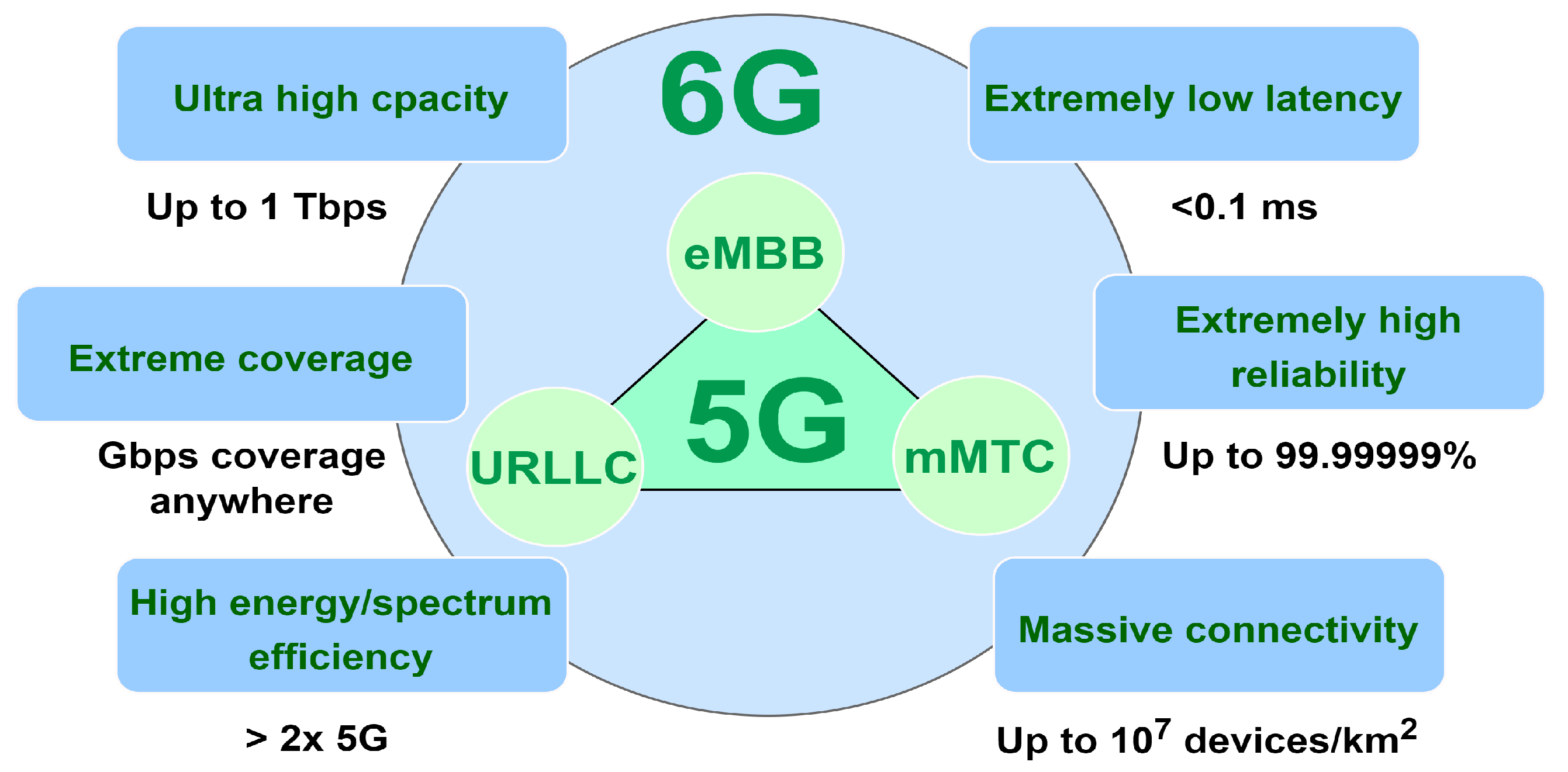
| Aspect | 5G | 6G |
|---|---|---|
| Year | 2020 | 2030 |
| Peak data rate (per device) | 10 Gbps | 1 Tbps |
| Maximum frequency | 300 GHz | 10 THz |
| Downlink data rate | 20 Gbps | 1 Tbps |
| Uplink data rate | 10 Gbps | 1 Tbps |
| Latency | 1 ms | 100 s |
| Jitter | not specified | 1 s |
| Mobility | 500 km/h | 1000 km/h |
| Maximum bandwidth | 1 GHz | 100 GHz |
| Density of devices | devices/km | devices/km |
| Area traffic capacity | 10 Mb/s/m | 1 Gb/s/m |
| Peak spectral efficiency | 30 b/s/Hz | 100 b/s/Hz |
| Reliability | > | > |
| Average Required Capacity (Gbps) | ||||||||||
|---|---|---|---|---|---|---|---|---|---|---|
| Split option | 1 | 2 | 3 | 4 | 5 | 6 | 7.3 | 7.2 | 7.1 | 8 |
| Downlink | 1 | 1 | 1 | 1 | 1 | 1.2 | 2 | 6 | 323 | 885 |
| Uplink | 1 | 1 | 1 | 1 | 1 | 1.2 | 3.2 | 2 | 323 | 885 |
| Fronthaul Technology | Throughput | Latency | Cost | Distance | Topology |
|---|---|---|---|---|---|
| P2P Fiber | 1000 Gbps | Very low | High | 100 km | P2P |
| PON | 40 Gbps | Very low | Low | 40 km | P2mP |
| xDSL | 100 Mbps | Very High | Very low | 500 m | P2P |
| FSO | 10 Gbps | Very Low | Low | 5 km | P2P, P2mP |
| Microwave | 1 Gbps | Moderate | Moderate | 10 km | P2P, P2mP |
| mmWaves | 10 Gbps | Moderate | High | 1 km | P2P, P2mP |
| Notation | Description |
|---|---|
| B | A set of potential locations where the BBU pool, the OLT, and the AWG can be located |
| P | A set of candidate locations for splitters |
| N | A set of RRH locations |
| L | A set of BBUs |
| O | A set of OLTs |
| Number of locations available for BBU pool placement | |
| Number of BBUs | |
| Number of OLTs | |
| Number of AWGs | |
| Number of splitters | |
| Number of RRHs, where =|N| | |
| The maximum number of BBU pools | |
| The maximum number of RRHs that can be served by one BBU | |
| The distance between the BBU pool and the power splitter (the feeder fiber) | |
| The distance between the power splitter and the RRH (the distributed fiber) | |
| The maximum allowed distance for the distributed fiber | |
| The maximum allowed distance for the feeder fiber | |
| Number of splits for the power splitter (splitting ratio) | |
| The cost of fiber optic cable per meter (material and deployment cost) | |
| The cost of the OLT | |
| The power splitter cost | |
| The BBU cost | |
| The RRH cost | |
| The BBU pool cost | |
| The cost of AWG | |
| Operations and maintenance cost | |
| Site rental cost | |
| E | Energy consumption cost |
| Energy consumption of the BBU | |
| Energy consumption of the OLT | |
| Energy consumption of the RRH | |
| Energy consumption of the cooling system | |
| TWDM-OPON downlink capacity | |
| TWDM-PON uplink capacity | |
| The capacity required by each RRH for downlink | |
| The capacity required by each RRH for uplink |
| Variable | Description |
|---|---|
| Equals 1 if the bth BBU pool is used; 0 otherwise | |
| Equals 1 if the nth RRH is active; 0 otherwise. | |
| Equals 1 if the pth power splitter is active; 0 otherwise. | |
| Equals 1 f the bth BBU pool and the pth power splitter are connected; 0 otherwise | |
| Equals 1 if the pth power splitter and the nth RRH are connected; 0 otherwise. |
| Parameter | Value |
|---|---|
| USD 20 per m (USD 4 for purchase and 16 for trenching) [25] | |
| 2500, where is the number of wavelengths (here 4) | |
| USD 75000 [25] | |
| USD 3600 [27] | |
| USD 3500 [25] | |
| [51] | |
| USD (30, 50, 100) for (1:4, 1:8, 1:16) splitting ratios, respectively [25] | |
| 10% of equipment cost [37] | |
| USD 8000 per year per RRH [25] | |
| E | USD 0.15 per Watt |
| 100 W [25] | |
| 155 W [25] | |
| 104 W [25] | |
| 500 W [25] | |
| 10 RRHs | |
| Mutation probability | 0.05 |
| Crossover probability | 0.8 |
| Number of replications | 100 |
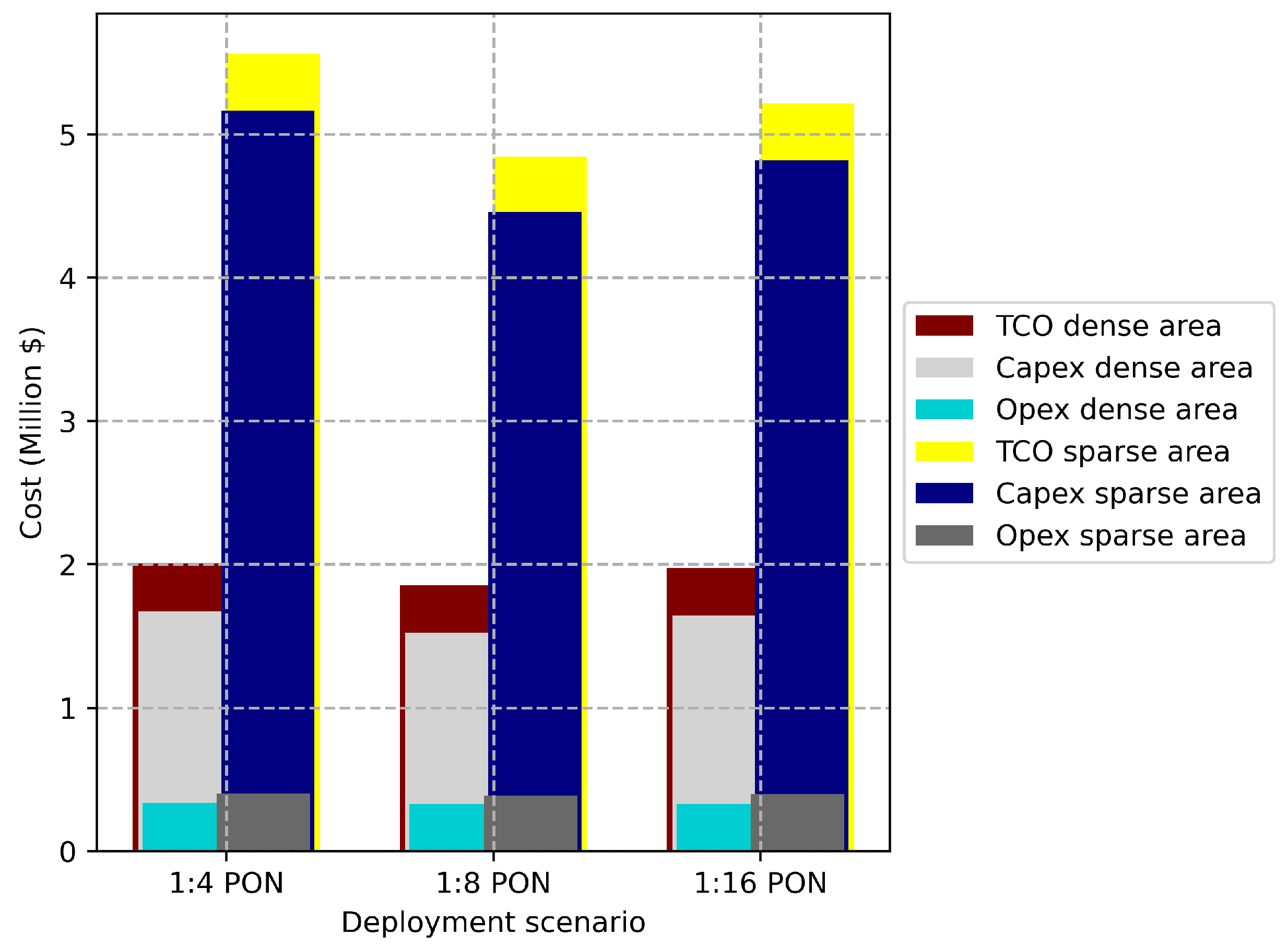
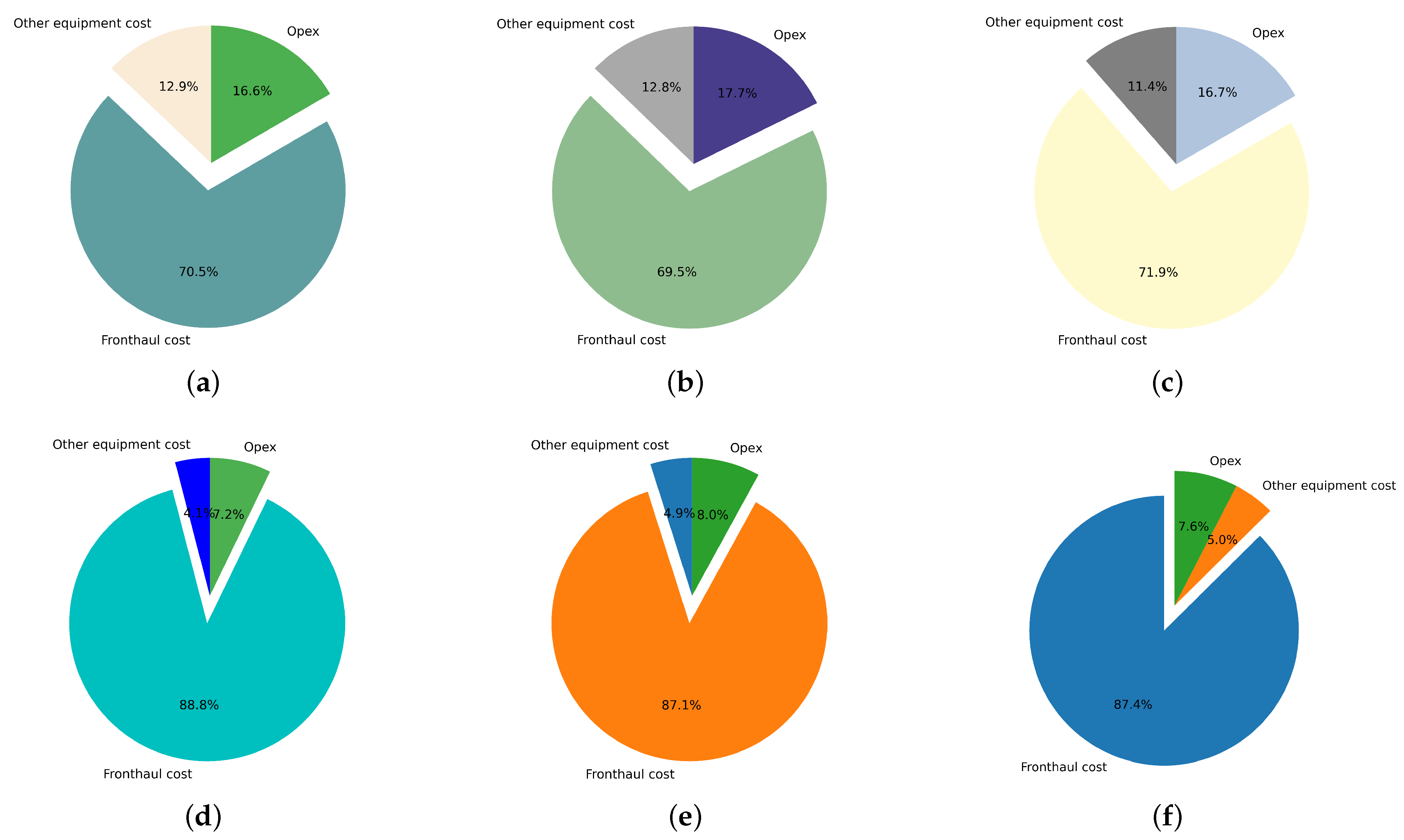
| Deployment Area | Dense | Sparse | ||||
|---|---|---|---|---|---|---|
| PON architecture | 1:4 | 1:8 | 1:16 | 1:4 | 1:8 | 1:16 |
| Fronthaul cost (USD) | 14.15 | 12.88 | 14.12 | 42.39 | 42.21 | 45.60 |
| Opex (USD) | 3.33 | 3.29 | 3.28 | 3.99 | 3.96 | 3.86 |
| Other equipment cost (USD) | 2.59 | 2.37 | 2.25 | 2.59 | 2.37 | 2.25 |
Publisher’s Note: MDPI stays neutral with regard to jurisdictional claims in published maps and institutional affiliations. |
© 2022 by the authors. Licensee MDPI, Basel, Switzerland. This article is an open access article distributed under the terms and conditions of the Creative Commons Attribution (CC BY) license (https://creativecommons.org/licenses/by/4.0/).
Share and Cite
Fayad, A.; Cinkler, T.; Rak, J.; Jha, M. Design of Cost-Efficient Optical Fronthaul for 5G/6G Networks: An Optimization Perspective. Sensors 2022, 22, 9394. https://doi.org/10.3390/s22239394
Fayad A, Cinkler T, Rak J, Jha M. Design of Cost-Efficient Optical Fronthaul for 5G/6G Networks: An Optimization Perspective. Sensors. 2022; 22(23):9394. https://doi.org/10.3390/s22239394
Chicago/Turabian StyleFayad, Abdulhalim, Tibor Cinkler, Jacek Rak, and Manish Jha. 2022. "Design of Cost-Efficient Optical Fronthaul for 5G/6G Networks: An Optimization Perspective" Sensors 22, no. 23: 9394. https://doi.org/10.3390/s22239394