
Treatment of Extended Kalman Filter Implementations for the Gyroless Star Tracker


Abstract
:1. Introduction
- Novel implementation of the multiplicative EKF for the case of the gyroless star tracker.
- Analysis employs both simulation and real night sky testing. Provides a case example of the novel approach of star tracker testing by [33].
- Enabling more compact and lower power attitude determination systems.
- Improving attitude estimation accuracy and precision, a topic of interest for not only satellite attitude control but SSA applications.
- Reducing bias to attitude and rate estimates.
2. Model and Methods
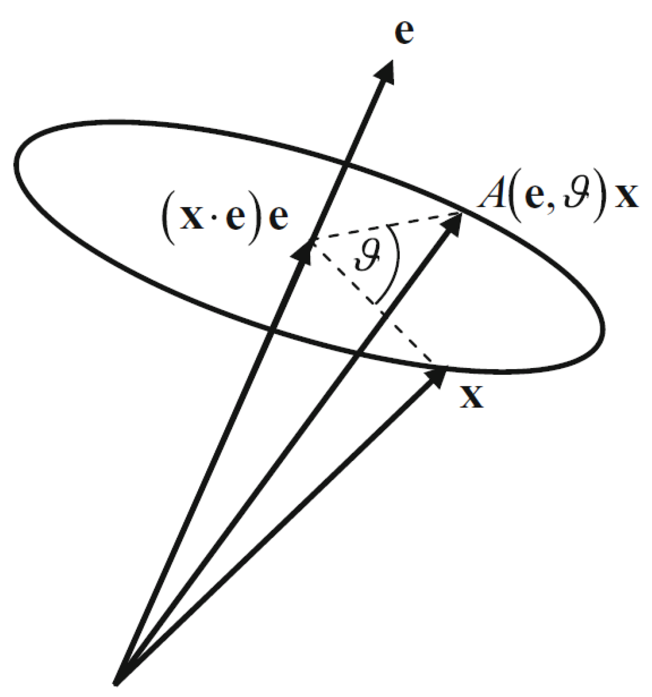
2.1. Attitude Definitions
2.2. Star Tracker Model
2.3. Extended Kalman Filter Model
2.3.1. State-Based Estimation
2.3.2. State Error Estimation
3. Results and Discussion
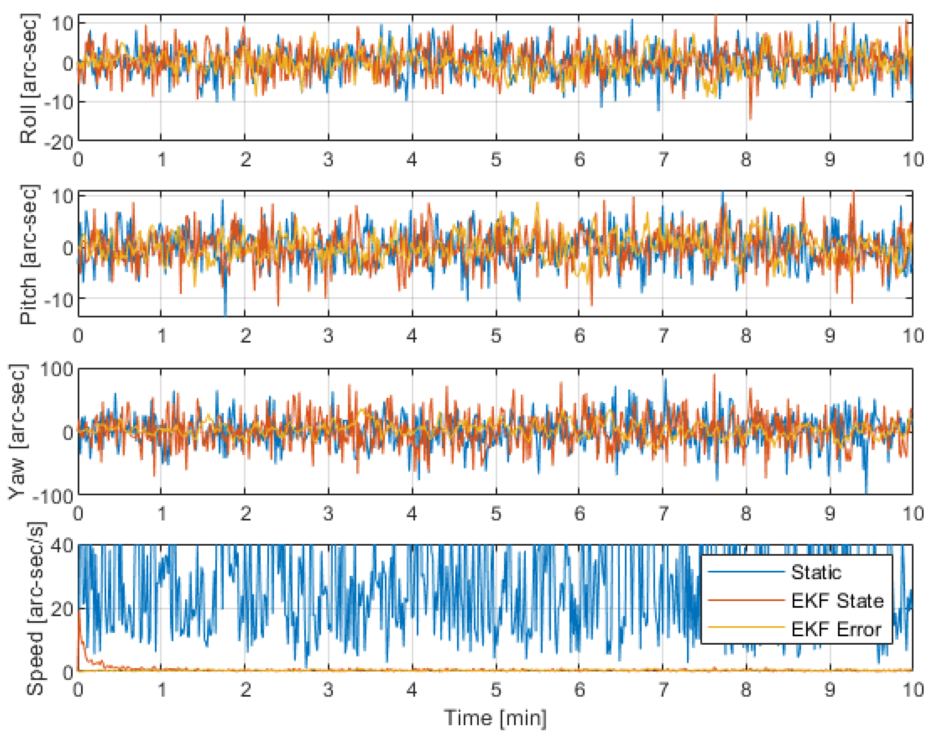
3.1. Simulations
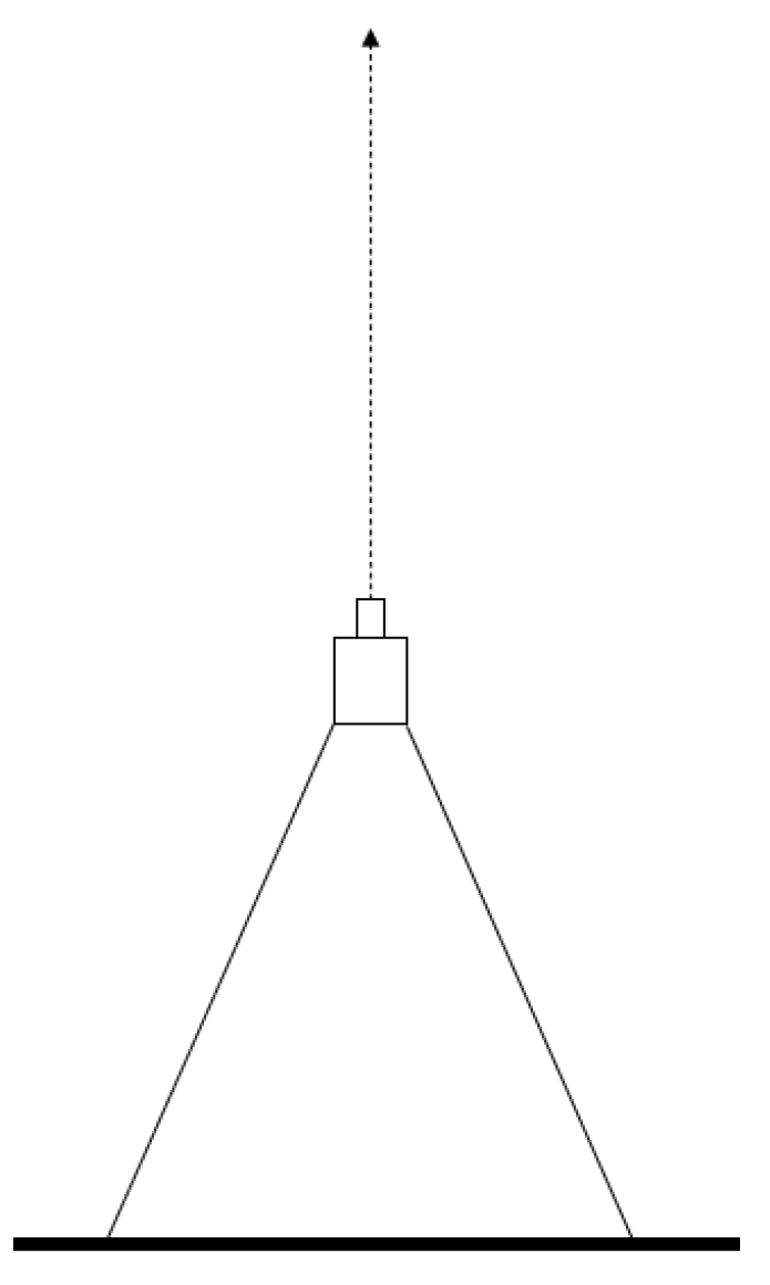
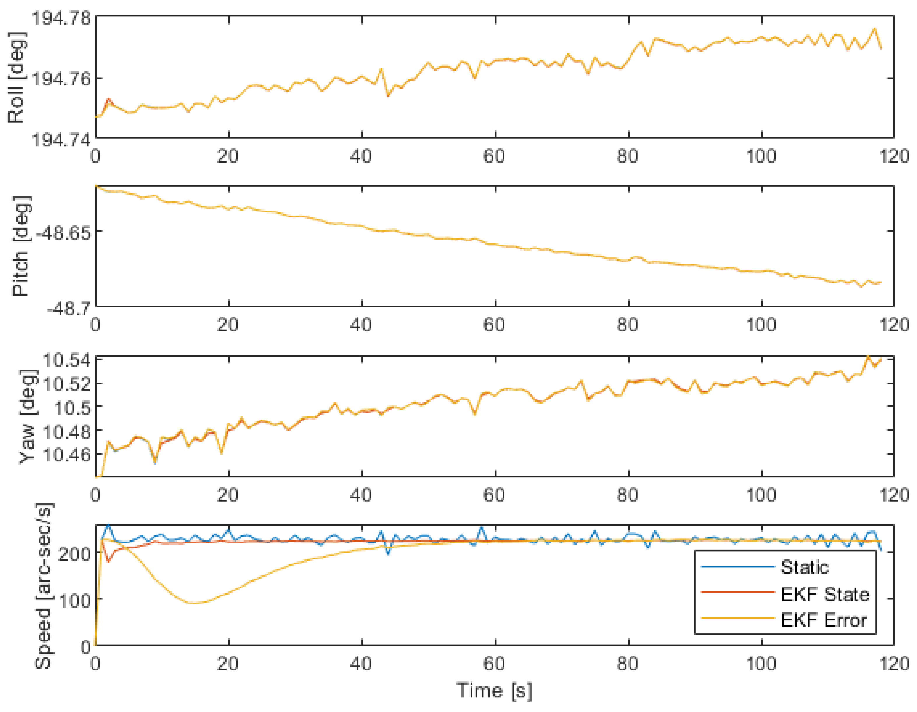
3.2. Real Night Sky
4. Conclusions
Author Contributions
Funding
Acknowledgments
Conflicts of Interest
References
- Kalman, R.E. A new approach to linear filtering and prediction problems. J. Fluids Eng. Trans. ASME 1960, 82, 35–45. [Google Scholar] [CrossRef] [Green Version]
- McLean, J.D.; Schmidt, S.F.; McGee, L.A. Optimal Filtering and Linear Prediction Applied to a Midcourse Navigation System for the Circumlunar Mission; Technical Report; NASA-AMES Research Center: Moffett Field, CA, USA, 1961. [Google Scholar]
- Smith, G.L.; Schmidt, S.F.; McGee, L.A. Application of Statistical Filter Theory to the Optimal Estimation of Position and Velocity on Board a Circumlunar Vehicle; Technical Report; NASA-AMES Research Center: Moffett Field, CA, USA, 1962. [Google Scholar]
- Farrell, J.L. Attitude Determination by Kalman Filtering. Autonatica 1970, 6, 419–430. [Google Scholar] [CrossRef]
- Pauling, D.C.; Jackson, D.B.; Brown, C.D. SPARS algorithms and simulation results. In Proceedings of the Symposium on Spacecraft Attitude Determination, El Segundo, CA, USA, 30 September–2 October 1969; pp. 293–316. [Google Scholar]
- Gai, E.; Daly, K.; Harrison, J.; Lemos, L. Star-Sensor-Based Satellite Attitude/Attitude Rate Estimator. J. Guid. Control Dyn. 1985, 8, 560–565. [Google Scholar] [CrossRef]
- Challa, M.; Natanson, G.A.; Baker, D.E.; Deutschmann, J.K. Advantages of Estimating Rate Corrections During Dynamic Propagation of Spacecraft Rates-Applications to Real-Time Attitude Determination of SAMPEX. In Proceedings of the Flight Mechanics/Estimation Theory Symposium, Greenbelt, MD, USA, 17–19 May 1994; pp. 481–495. [Google Scholar]
- Chu, D.; Harvie, E. Accuracy of the ERBS Definitive Attitude Determination System in the Presence of Propagation Noise. In Proceedings of the Flight Mechanics/Estimation Theory Symposium, Greenbelt, MD, USA, 22–24 May 1990; pp. 97–114. [Google Scholar]
- Crassidis, J.L.; Markley, F.L. Predictive Filtering for Attitude Estimation without Rate Sensors. J. Guid. Control Dyn. 1997, 20, 522–527. [Google Scholar] [CrossRef] [Green Version]
- Hajiyev, C.; Guler, D.C. Review on gyroless attitude determination methods for small satellites. Prog. Aerosp. Sci. 2017, 90, 54–66. [Google Scholar] [CrossRef]
- Shuster, M.D. Kalman Filtering of Spacecraft Attitude and the QUEST Model. J. Astronaut. Sci. 1990, 38, 377–393. [Google Scholar]
- Leffens, E.J.; Markley, F.L.; Shuster, M.D. Kalman filtering for spacecraft attitude estimation. J. Guid. Control Dyn. 1982, 5, 417–429. [Google Scholar] [CrossRef]
- Crassidis, J.L.; Markley, F.L. Unscented filtering for spacecraft attitude estimation. J. Guid. Control Dyn. 2003, 26, 536–542. [Google Scholar] [CrossRef] [Green Version]
- Cheng, Y.; Crassidis, J.L.; Markley, F.L. Attitude Estimation for Large Field-of-View Sensors. J. Astronaut. Sci. 2006, 54, 433–448. [Google Scholar] [CrossRef] [Green Version]
- Markley, F.L.; Crassidis, J.L. Filtering for Attitude Estimation and Calibration. In Fundamentals of Spacecraft Attitude Determination and Control, 1st ed.; Springer Science and Business Media: Berlin/Heidelberg, Germany, 2014; pp. 235–343. [Google Scholar]
- Darling, J.E.; Houtz, N.; Frueh, C.; Demars, K.J. Recursive filtering of star tracker data. In Proceedings of the AIAA/AAS Astrodynamics Specialist Conference, Long Beach, CA, USA, 13–16 September 2016; pp. 5672–5695. [Google Scholar] [CrossRef]
- Li, J.; Wei, X.; Zhang, G. An extended Kalman filter-based attitude tracking algorithm for star sensors. Sensors 2017, 17, 1921. [Google Scholar] [CrossRef] [PubMed]
- Tan, N.D.; Vinh, T.Q.; Tuyen, B.T. A new approach for small satellite gyroscope and star tracker fusion. Indian J. Sci. Technol. 2016, 9, 1–7. [Google Scholar] [CrossRef]
- Fan, C.; Meng, Z.; Liu, X. Multiplicative quaternion extended consensus Kalman filter for attitude and augmented state estimation. In Proceedings of the Chinese Control Conference, CCC, Chengdu, China, 27–29 July 2016; pp. 8043–8048. [Google Scholar] [CrossRef]
- Lee, D.; Vukovich, G.; Lee, R. Robust Adaptive Unscented Kalman Filter for Spacecraft Attitude Estimation Using Quaternion Measurements. J. Aerosp. Eng. 2017, 30, 04017009. [Google Scholar] [CrossRef]
- Grewal, M.; Shiva, M. Application of Kalman filtering to gyroless attitude determination and control system for environmental satellites. In Proceedings of the 1995 34th IEEE Conference on Decision and Control, New Orleans, LA, USA, 13–15 December 1995; Volume 2, pp. 1544–1552. [Google Scholar]
- Dave, S.; Clark, R.; Lee, R.S. RSOnet: An Image-Processing Framework for a Dual-Purpose Star Tracker as an Opportunistic Space Surveillance Sensor. Sensors 2022, 22, 5688. [Google Scholar] [CrossRef] [PubMed]
- Tetlow, M.R.; Chin, T. Robust Attitude Estimation to Support Space Monitoring Using Nano-Satellites. In Proceedings of the AIAA SPACE 2014 Conference and Exposition, San Diego, CA, USA, 4–7 August 2014; p. 4293. [Google Scholar]
- Gaoxiang, O.; Wenliang, L.; Pingke, D.; Guocan, Z. Attitude and Angle Rate Determination of Gyroless Spacecraft Based on SVD Kalman Filter Only Using Star Sensor. In Proceedings of the 2021 33rd Chinese Control and Decision Conference (CCDC), Kunming, China, 22–24 May 2021; pp. 5256–5260. [Google Scholar]
- Leeghim, H.; Bang, H.; Lee, C.Y. Angular rate and alignment estimation for gyroless spacecraft by only star trackers. Int. J. Control Autom. Syst. 2018, 16, 2235–2243. [Google Scholar] [CrossRef]
- Ding, Y.; Zhao, X.; Zhang, Z.; Cai, W.; Yang, N.; Zhan, Y. Semi-supervised locality preserving dense graph neural network with ARMA filters and context-aware learning for hyperspectral image classification. IEEE Trans. Geosci. Remote. Sens. 2021, 60, 1–12. [Google Scholar] [CrossRef]
- Carron, A.; Todescato, M.; Carli, R.; Schenato, L.; Pillonetto, G. Machine learning meets Kalman filtering. In Proceedings of the 2016 IEEE 55th Conference on Decision and Control (CDC), Las Vegas, NV, USA, 12–14 December 2016; pp. 4594–4599. [Google Scholar]
- Zhang, S.T.; Wei, X.Y. Fuzzy adaptive Kalman filtering for DR/GPS. In Proceedings of the 2003 International Conference on Machine Learning and Cybernetics (IEEE Cat. No. 03EX693), Xi’an, China, 2–5 November 2003; Volume 5, pp. 2634–2637. [Google Scholar]
- Russo, A.; Lax, G. Using Artificial Intelligence for Space Challenges: A Survey. Appl. Sci. 2022, 12, 5106. [Google Scholar] [CrossRef]
- Suntup, M.; Cairns, I.; Critchley-Marrows, J.; Wu, X.; Albertson, D.; Guinane, J.; Jarvis, B. Implementation of a WFOV Star Tracker in CubeSat and Small Satellite Attitude Determination Systems. In Proceedings of the 43rd COSPAR Scientific Assembly, Sydney, Australia, 28 January–4 February 2021; Volume 43, p. 59. [Google Scholar]
- Critchley-Marrows, J.; Wu, X. Investigation into Integrated Attitude Determination in High-Precision CubeSats. In Proceedings of the 68th International Astronautical Congress, Adelaide, Australia, 25–29 September 2017; pp. 1–5. [Google Scholar]
- Critchley-Marrows, J.; Wu, X. Investigation into Star Tracker Algorithms using Smartphones with Application to High-Precision Pointing CubeSats. Trans. Jpn. Soc. Aeronaut. Space Sci. 2019, 17, 327. [Google Scholar] [CrossRef]
- Jarvis, B.; Guinane, J.; Wu, X.; Critchley-Marrows, J. Development of a Low-Cost Testing Methodology for Star Trackers. In Proceedings of the 19th Australian Space Research Conference, Adelaide, Australia, 30 September–2 October 2020; pp. 1–14. [Google Scholar]
- Chou, J.C. Quaternion Kinematic and Dynamic Differential Equations. IEEE Trans. Robot. Autom. 1992, 8, 53–64. [Google Scholar] [CrossRef]
- FLIR. Technical Reference—FLIR Blackfly S. Available online: https://www.eureca.de/files/pdf/optoelectronics/flir/BFS-U3-50S5-BD2-Technical-Reference.pdf (accessed on 1 August 2022).
- Scorpion Vision Limited. Specification Sheet—S-Mount 25mm F1.7 Lens–SVL-IR2517B5M. Available online: https://files.ecommercedns.uk/230067/ffc50f57ca9f2b26564af2e7b3343768.pdf (accessed on 1 August 2022).
- Farenkopf, R.L. Analytic steady-state accuracy solutions for two common spacecraft attitude estimators. J. Guid. Navig. Control 1978, 1, 282–284. [Google Scholar] [CrossRef]
- Guinane, J.; Jarvis, B.; Suntup, M.; Wu, X.; Critchley-Marrows, J.; Cairns, I.H. Assessing the viability of a wide field of view based stellar gyroscope. In Proceedings of the 18th Australian Space Research Conference, Adelaide, Australia, 30 September–2 October 2019; pp. 109–120. [Google Scholar]


| States | |
| Propagation Update | |
| Measurement Update | |
| States | |
| Propagation Update | |
| Measurement Update | |
| Parameter | Measure | LLS | EKF State | EKF State Error |
|---|---|---|---|---|
| Roll | Error [arc-sec] | 0.04 | 0.01 | 0.12 |
| Standard Deviation [arc-sec] | 3.59 | 2.60 | 3.26 | |
| Pitch | Error [arc-sec] | 0.02 | 0.05 | 0.13 |
| Standard Deviation [arc-sec] | 3.65 | 2.53 | 2.91 | |
| Yaw | Error [arc-sec] | 0.60 | 0.46 | 0.20 |
| Standard Deviation [arc-sec] | 25.86 | 7.88 | 12.93 | |
| Speed | Error [arc-sec/s] | 30.63 | 0.12 | 0.4 |
| Standard Deviation [arc-sec/s] | 21.3 | 0.31 | 0.18 |
| Parameter | Measure | LLS | EKF State | EKF State Error |
|---|---|---|---|---|
| Roll | Residual [arc-sec] | 28.49 | 28.32 | 28.51 |
| Standard Deviation [arc-sec] | 8.34 | 8.43 | 8.34 | |
| Pitch | Residual [arc-sec] | 66.28 | 66.46 | 66.30 |
| Standard Deviation [arc-sec] | 6.26 | 6.33 | 6.27 | |
| Yaw | Residual [arc-sec] | 75.39 | 75.89 | 75.06 |
| Standard Deviation [arc-sec] | 27.87 | 26.18 | 27.74 | |
| Speed | Residual [arc-sec/s] | 10.17 | 0.70 | 1.50 |
| Standard Deviation [arc-sec/s] | 8.09 | 0.61 | 1.16 |
Publisher’s Note: MDPI stays neutral with regard to jurisdictional claims in published maps and institutional affiliations. |
© 2022 by the authors. Licensee MDPI, Basel, Switzerland. This article is an open access article distributed under the terms and conditions of the Creative Commons Attribution (CC BY) license (https://creativecommons.org/licenses/by/4.0/).
Share and Cite
Critchley-Marrows, J.J.R.; Wu, X.; Cairns, I.H. Treatment of Extended Kalman Filter Implementations for the Gyroless Star Tracker. Sensors 2022, 22, 9002. https://doi.org/10.3390/s22229002
Critchley-Marrows JJR, Wu X, Cairns IH. Treatment of Extended Kalman Filter Implementations for the Gyroless Star Tracker. Sensors. 2022; 22(22):9002. https://doi.org/10.3390/s22229002
Chicago/Turabian StyleCritchley-Marrows, Joshua J. R., Xiaofeng Wu, and Iver H. Cairns. 2022. "Treatment of Extended Kalman Filter Implementations for the Gyroless Star Tracker" Sensors 22, no. 22: 9002. https://doi.org/10.3390/s22229002