
Ultrasound Ultrafast Power Doppler Imaging with High Signal-to-Noise Ratio by Temporal Multiply-and-Sum (TMAS) Autocorrelation


Abstract
:1. Introduction
2. Theory
2.1. Conventional Power Doppler Imaging Using Zero-Lag Autocorrelation
2.2. Coherence-Based Power Doppler Imaging Using Higher-Lag Autocorrelation
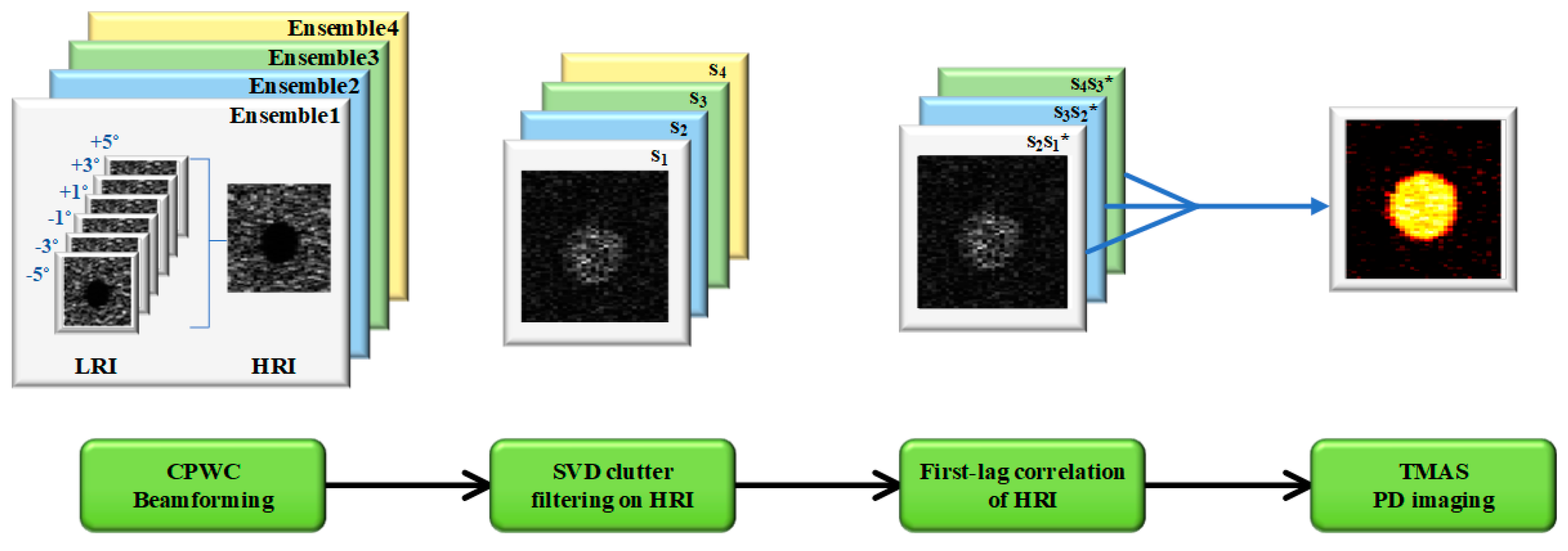
2.3. Higher-Lag Power Doppler Imaging Using Temporal Multiply-and-Sum (TMAS) Method
3. Methods
3.1. Simulation Setup
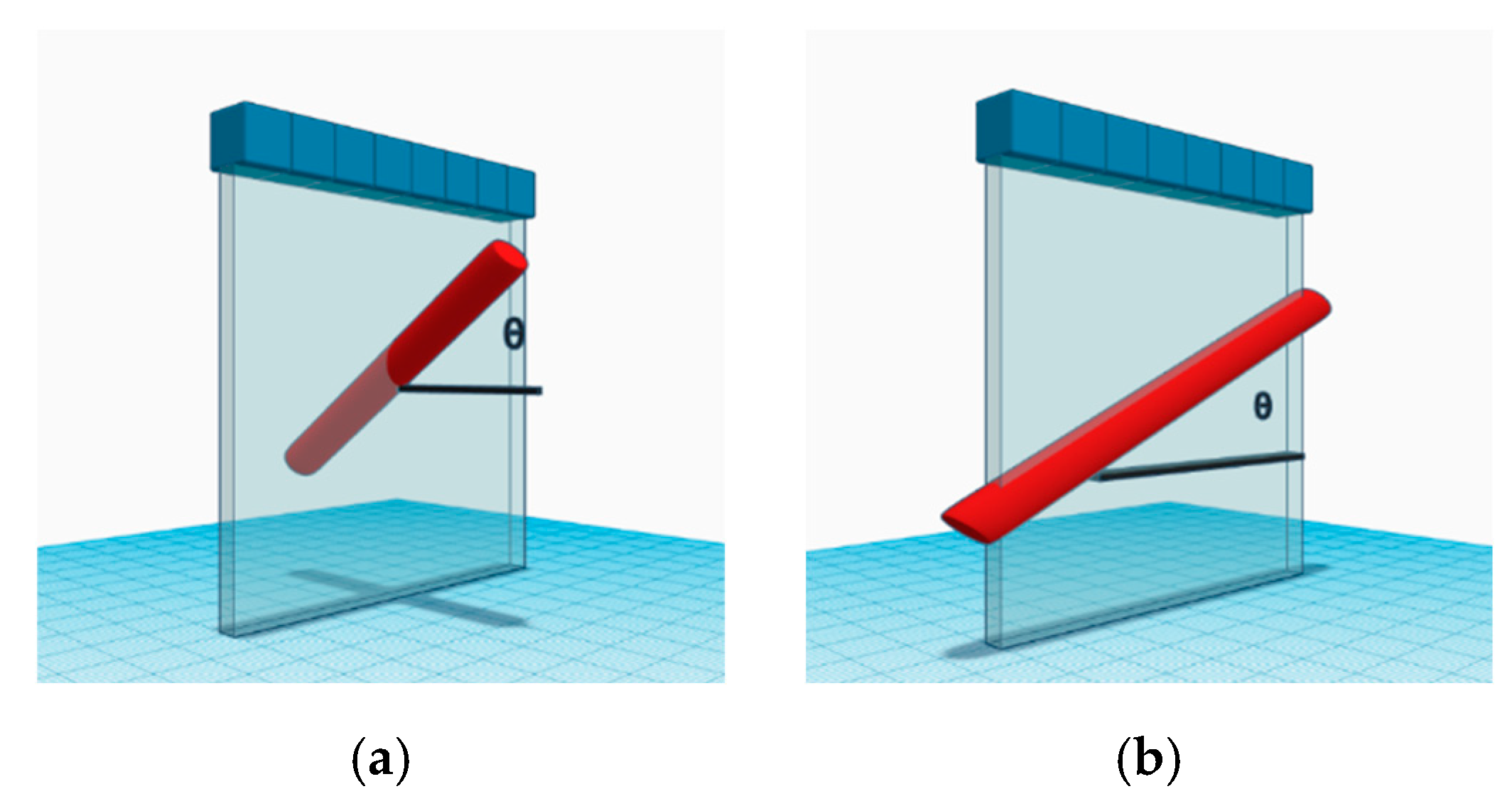
3.2. Experimental Setup
3.3. Quantitative Analysis
4. Results
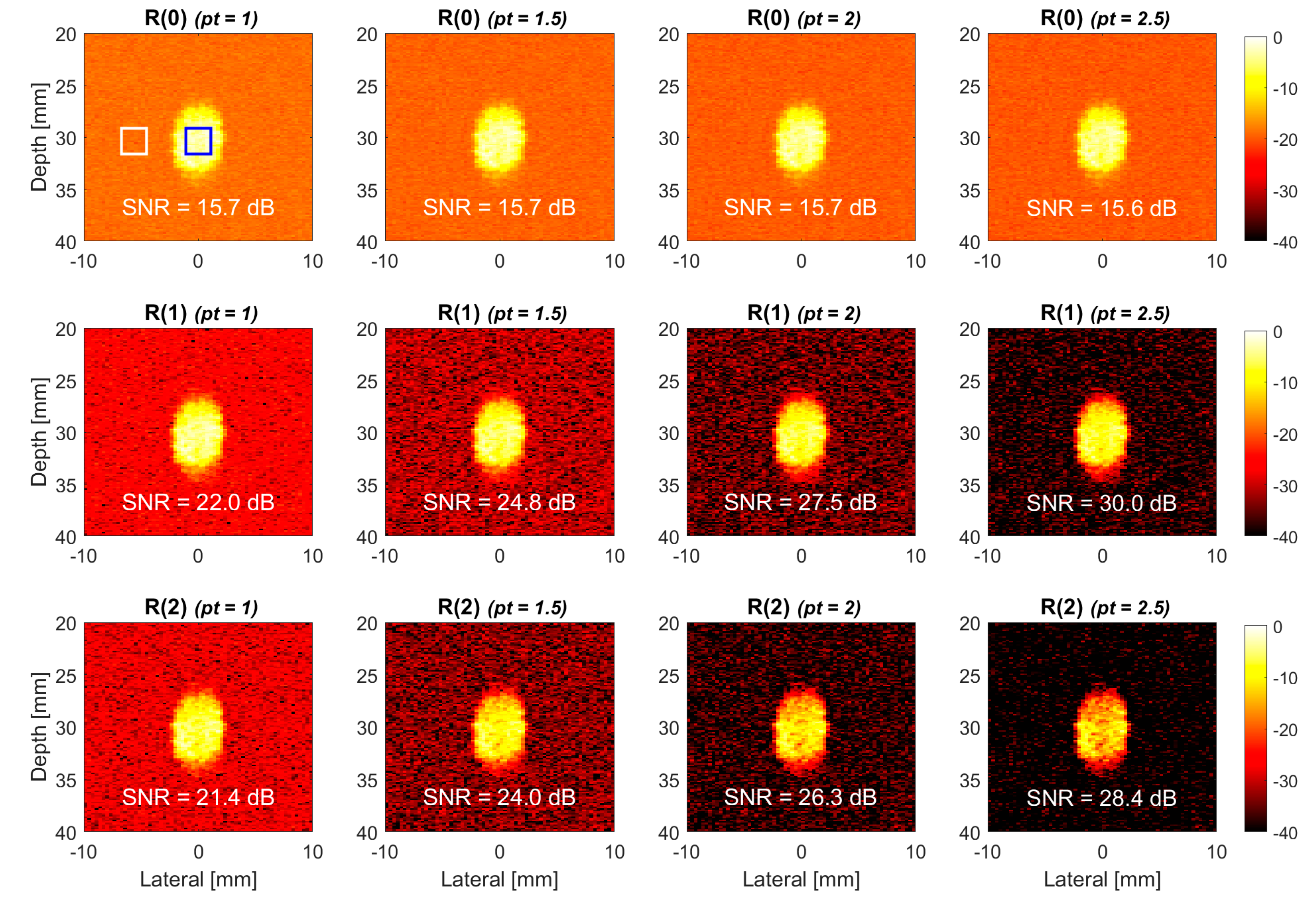
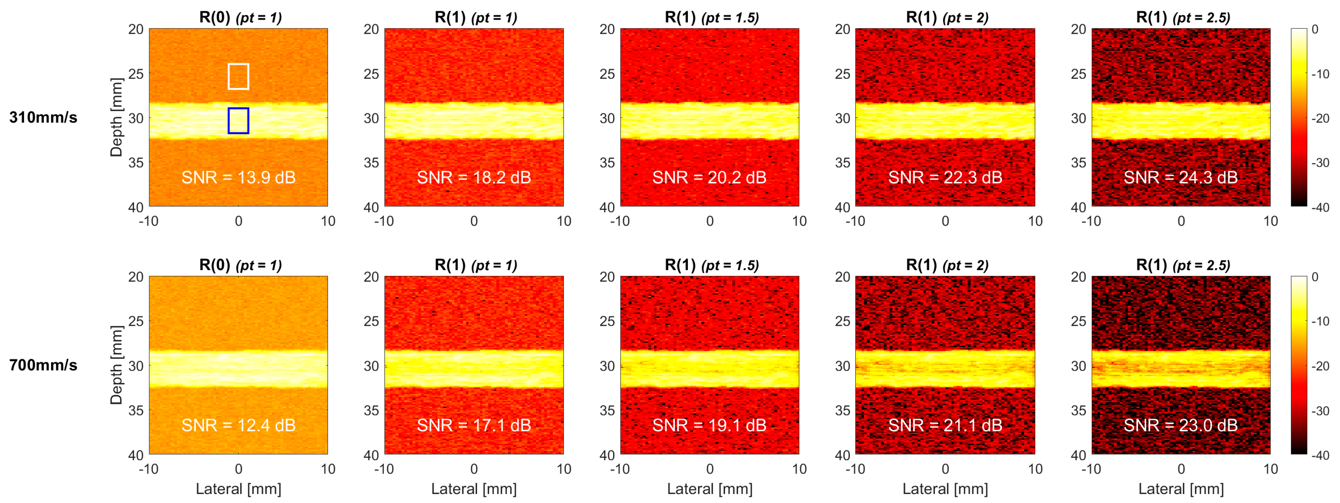
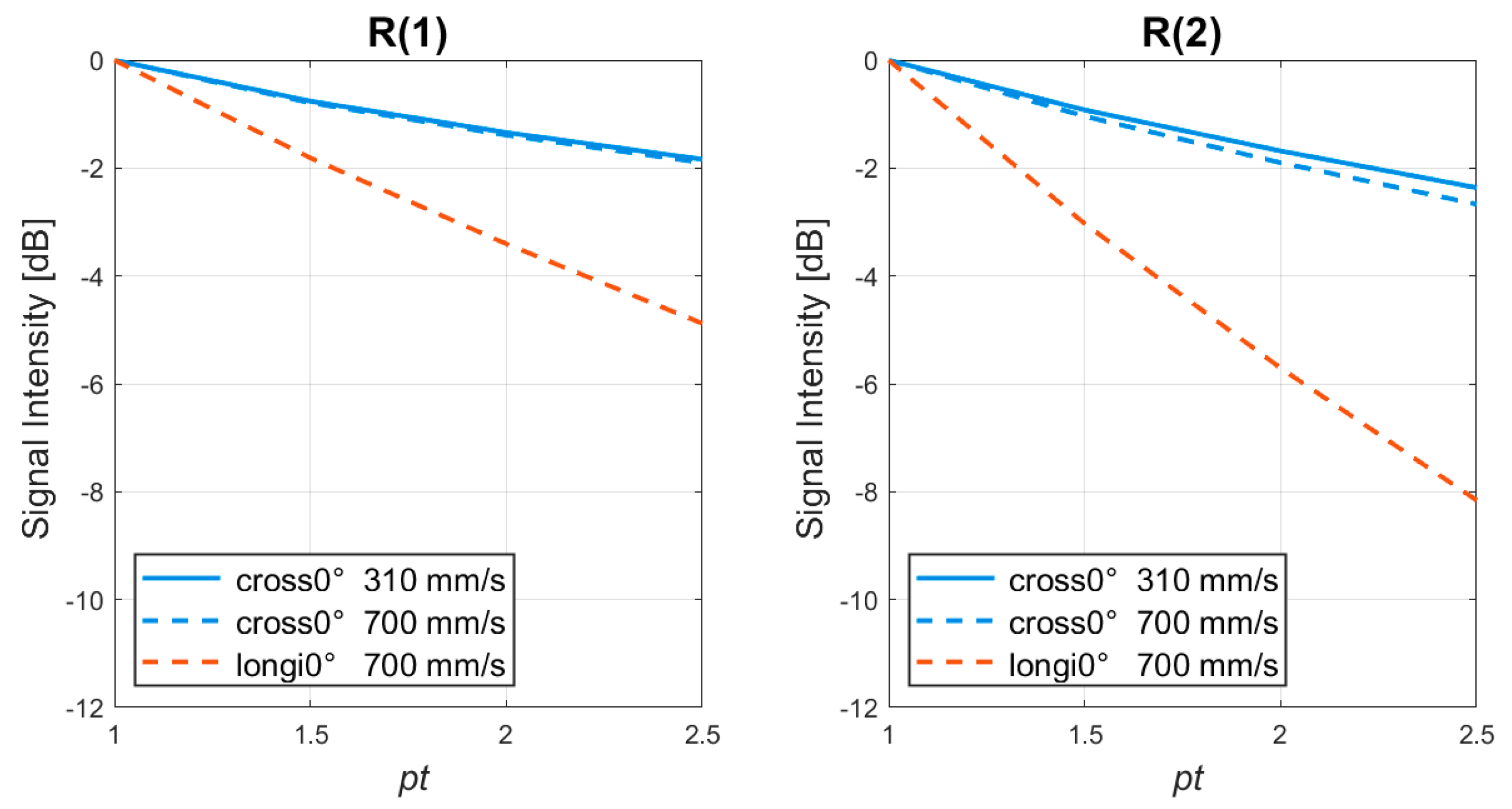
4.1. Simulations
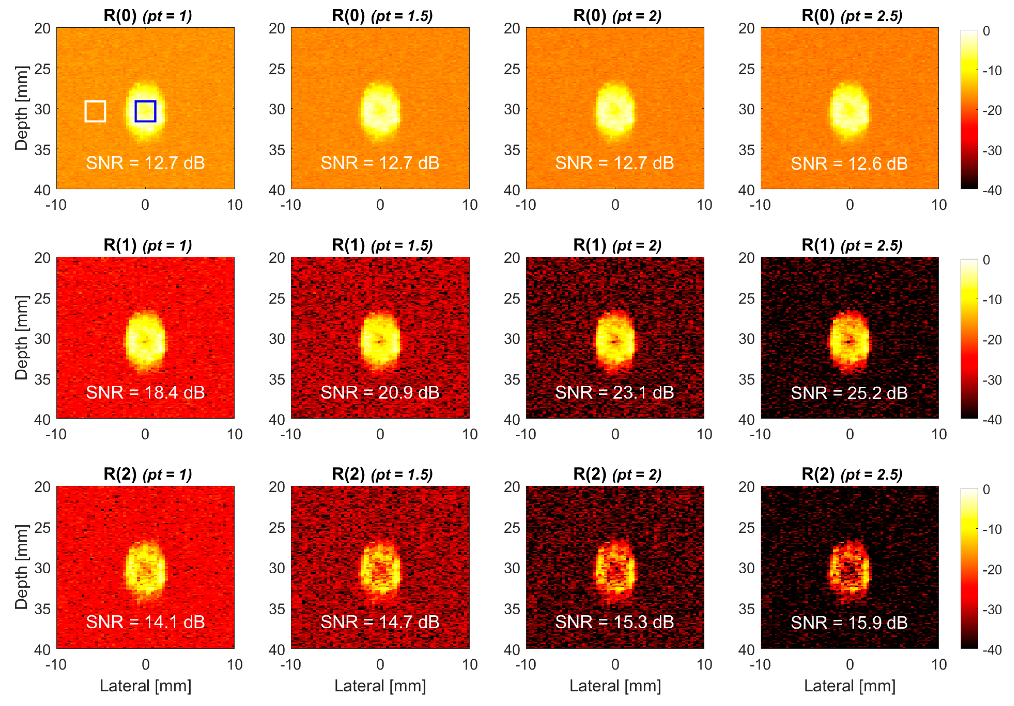
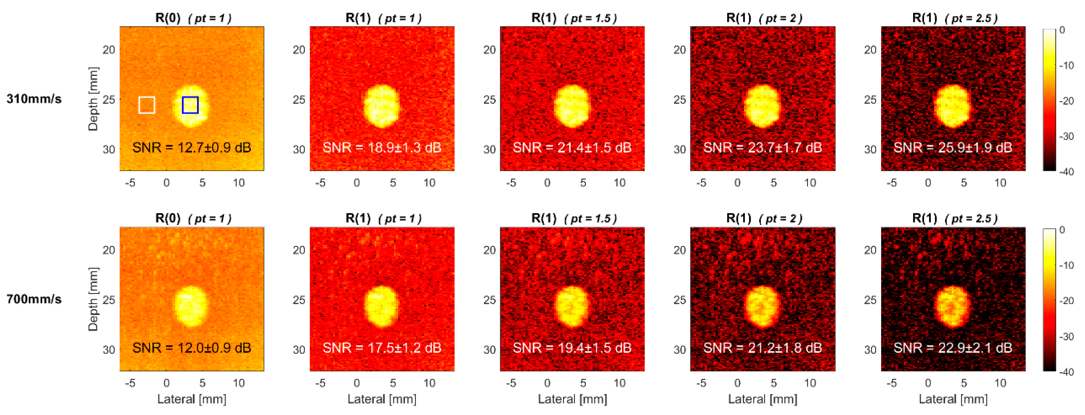
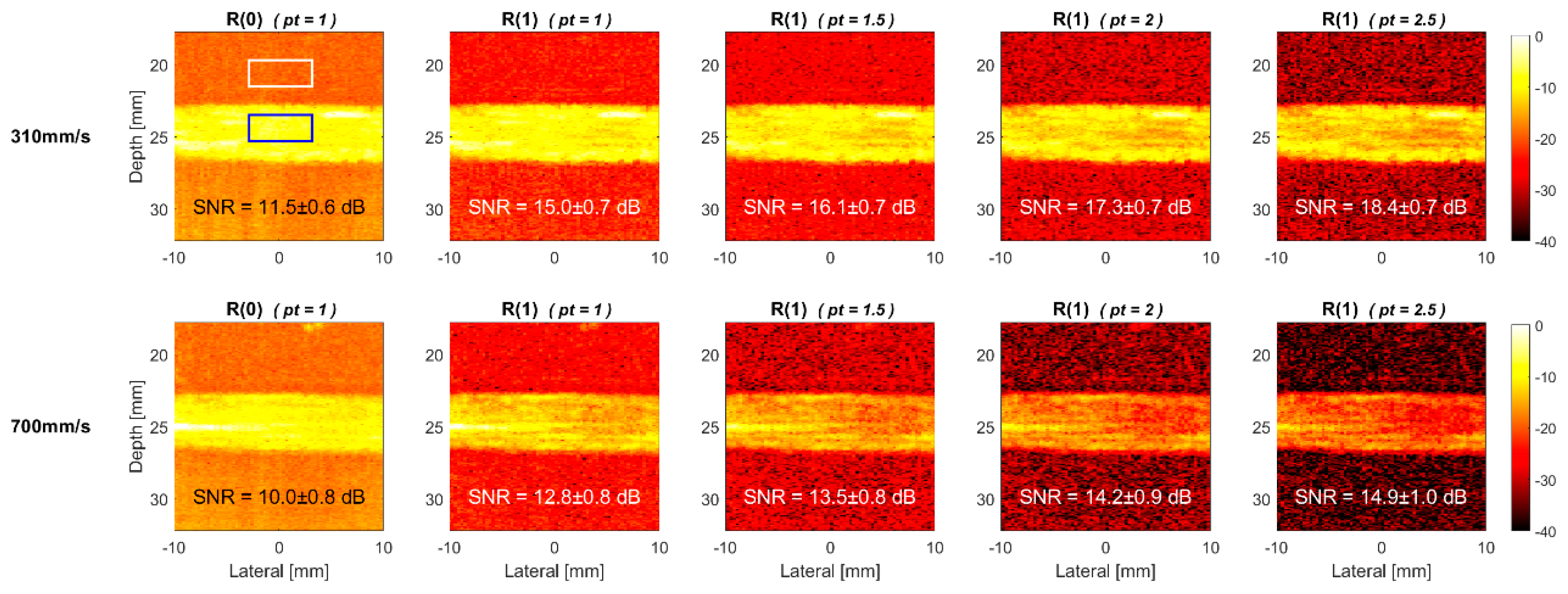
4.2. Experiments
5. Discussion and Conclusions
Author Contributions
Funding
Institutional Review Board Statement
Informed Consent Statement
Data Availability Statement
Acknowledgments
Conflicts of Interest
References
- So, H.; Chen, J.; Yiu, B.; Yu, A. Medical Ultrasound Imaging: To GPU or Not to GPU? IEEE Micro 2011, 31, 54–65. [Google Scholar] [CrossRef] [Green Version]
- Sandrin, L.; Catheline, S.; Tanter, M.; Hennequin, X.; Fink, M. Time-resolved pulsed elastography with ultrafast ultrasonic imaging. Ultrason. Imaging 1999, 21, 259–272. [Google Scholar] [CrossRef] [PubMed]
- Tanter, M.; Fink, M. Ultrafast imaging in biomedical ultrasound. IEEE Trans. Ultrason. Ferroelectr. Freq. Control 2014, 61, 102–119. [Google Scholar] [CrossRef] [PubMed]
- Montaldo, G.; Tanter, M.; Bercoff, J.; Benech, N.; Fink, M. Coherent plane-wave compounding for very high frame rate ultrasonography and transient elastography. IEEE Trans. Ultrason. Ferroelectr. Freq. Control 2009, 56, 489–506. [Google Scholar] [CrossRef] [PubMed]
- Zhang, Y.; Li, H.; Lee, W.N. Imaging heart dynamics with ultrafast cascaded-wave ultrasound. IEEE Trans. Ultrason. Ferroelectr. Freq. Control 2019, 66, 1465–1479. [Google Scholar] [CrossRef]
- Bercoff, J.; Montaldo, G.; Loupas, T.; Savery, D.; Mézière, F.; Fink, M.; Tanter, M. Ultrafast compound Doppler imaging: Providing full blood flow characterization. IEEE Trans. Ultrason. Ferroelectr. Freq. Control 2011, 58, 134–147. [Google Scholar] [CrossRef]
- Osmanski, B.F.; Pernot, M.; Montaldo, G.; Bel, A.; Messas, E.; Tanter, M. Ultrafast Doppler imaging of blood flow dynamics in the myocardium. IEEE Trans. Med. Imaging 2012, 31, 1661–1668. [Google Scholar] [CrossRef]
- Ekroll, I.K.; Swillens, A.; Segers, P.; Dahl, T.; Torp, H.; Lovstakken, L. Simultaneous quantification of flow and tissue velocities based on multi-angle plane wave imaging. IEEE Trans. Ultrason. Ferroelectr. Freq. Control 2013, 60, 727–738. [Google Scholar] [CrossRef]
- Mace, E.; Montaldo, G.; Osmanski, B.F.; Cohen, I.; Fink, M.; Tanter, M. Functional ultrasound imaging of the brain: Theory and basic principles. IEEE Trans. Ultrason. Ferroelectr. Freq. Control 2013, 60, 492–506. [Google Scholar] [CrossRef]
- Ricci, S.; Bassi, L.; Tortoli, P. Real-time vector velocity assessment through multigate Doppler and plane waves. IEEE Trans. Ultrason. Ferroelectr. Freq. Control 2014, 61, 314–324. [Google Scholar] [CrossRef]
- Yiu, B.Y.S.; Yu, A.C.H. Least-squares multi-angle Doppler estimators for plane-wave vector flow imaging. IEEE Trans. Ultrason. Ferroelectr. Freq. Control 2016, 63, 1733–1744. [Google Scholar] [CrossRef]
- Ekroll, I.K.; Voormolen, M.M.; Standal, O.K.-V.; Rau, J.M.; Lovstakken, L. Coherent compounding in Doppler imaging. IEEE Trans. Ultrason. Ferroelectr. Freq. Control 2015, 62, 1634–1643. [Google Scholar] [CrossRef] [PubMed]
- Leow, C.H.; Bazigou, E.; Eckersley, R.J.; Yu, A.C.H.; Weinberg, P.D.; Tang, M.X. Flow velocity mapping using contrast enhanced high-frame-rate plane wave ultrasound and image tracking: Methods and initial in vitro and in vivo evaluation. Ultrasound Med. Biol. 2015, 41, 2913–2925. [Google Scholar] [CrossRef] [PubMed] [Green Version]
- Rubin, J.M.; Bude, R.O.; Carson, P.L.; Bree, R.L.; Adler, R.S. Power Doppler US: A potentially useful alternative to mean frequency-based color Doppler US. Radiology 1994, 190, 853–856. [Google Scholar] [CrossRef] [PubMed]
- Bude, R.O.; Rubin, J.M. Power Doppler sonography. Radiology 1996, 200, 21–23. [Google Scholar] [CrossRef]
- Li, Y.L.; Dahl, J.J. Coherent flow power Doppler (CFPD): Flow detection using spatial coherence beamforming. IEEE Trans. Ultrason. Ferroelectr. Freq. Control 2015, 62, 1022–1035. [Google Scholar] [CrossRef] [Green Version]
- Li, Y.L.; Hyun, D.; Abou-Elkacem, L.; Willmann, J.K.; Dahl, J.J. Visualization of small-diameter vessels by reduction of incoherent reverberation with coherent flow power Doppler. IEEE Trans. Ultrason. Ferroelectr. Freq. Control 2016, 63, 1878–1889. [Google Scholar] [CrossRef] [Green Version]
- Lediju, M.A.; Trahey, G.E.; Byram, B.C.; Dahl, J.J. Short-lag spatial coherence of backscattered echoes: Imaging characteristics. IEEE Trans. Ultrason. Ferroelectr. Freq. Control 2011, 58, 1377–1388. [Google Scholar] [CrossRef] [Green Version]
- Shen, C.C.; Chu, Y.C. DMAS Beamforming with Complementary Subset Transmit for Ultrasound Coherence-Based Power Doppler Detection in Multi-Angle Plane-Wave Imaging. Sensors 2021, 14, 4856. [Google Scholar] [CrossRef]
- Kang, J.; Go, D.; Song, I.; Yoo, Y. Ultrafast Power Doppler Imaging Using Frame-Multiply-and-Sum-Based Nonlinear Compounding. IEEE Trans. Ultrason. Ferroelectr. Freq. Control 2021, 68, 453–464. [Google Scholar] [CrossRef]
- Matrone, G.; Savoia, A.S.; Caliano, G.; Magenes, G. The delay multiply and sum beamforming algorithm in ultrasound b-mode medical imaging. IEEE Trans. Med. Imaging 2015, 34, 940–949. [Google Scholar] [CrossRef]
- Polichetti, M.; Varray, F.; Béra, J.C.; Cachard, C.; Nicolas, B. Nonlinear beamformer based on p-th root compression—Application to plane wave ultrasound imaging. Appl. Sci. 2018, 8, 599. [Google Scholar] [CrossRef] [Green Version]
- Shen, C.C.; Hsieh, P.Y. Ultrasound baseband delay-multiply-and-sum (BB-DMAS) nonlinear beamforming. Ultrasonics 2019, 96, 165–174. [Google Scholar] [CrossRef]
- Huang, C.; Song, P.; Trzasko, J.D.; Gong, P.; Lok, U.W.; Tang, S.; Manduca, A.; Chen, S. Simultaneous Noise Suppression and Incoherent Artifact Reduction in Ultrafast Ultrasound Vascular Imaging. IEEE Trans. Ultrason. Ferroelectr. Freq. Control 2021, 68, 2075–2085. [Google Scholar] [CrossRef]
- Stanziola, A.; Leow, C.H.; Bazigou, E.; Weinberg, P.D.; Tang, M.X. ASAP: Super-contrast vasculature imaging using coherence analysis and high frame-rate contrast enhanced ultrasound. IEEE Trans. Med. Imaging 2018, 37, 1847–1856. [Google Scholar] [CrossRef] [Green Version]
- Leow, C.H.; Bush, N.L.; Stanziola, A.; Braga, M.; Shah, A.; Hernandez-Gil, J.; Long, N.J.; Aboagye, E.O.; Bamber, J.C.; Tang, M.X. 3-D microvascular imaging using high frame rate ultrasound and ASAP without contrast agents: Development and initial in vivo evaluation on nontumor and tumor models. IEEE Trans. Ultrason. Ferroelectr. Freq. Control 2019, 66, 939–948. [Google Scholar] [CrossRef] [Green Version]
- Huang, L.; Zhang, J.; Wei, X.; Jing, L.; He, Q.; Xie, X.; Wang, G.; Luo, J. Improved Ultrafast Power Doppler Imaging by Using Spatiotemporal Non-Local Means Filtering. IEEE Trans. Ultrason. Ferroelectr. Freq. Control 2022, 69, 1610–1624. [Google Scholar] [CrossRef]
- Charles, T.D.; Avinoam, B.Z.; Williams, R.; Sheeran, P.S.; Milot, L.; Loupas, T.; Adam, D.; Bruce, M.; Burns, P.N. Improved Contrast-Enhanced Power Doppler Using a Coherence-Based Estimator. IEEE Trans. Med. Imaging 2017, 36, 1901–1911. [Google Scholar]
- Demené, C.; Deffieux, T.; Pernot, M.; Osmanski, B.F.; Biran, V.; Gennisson, J.L.; Sieu, L.A.; Bergel, A.; Franqui, S.; Correas, J.M.; et al. Spatiotemporal clutter filtering of ultrafast ultrasound data highly increases Doppler and fUltrasound sensitivity. IEEE Trans. Med. Imaging 2015, 34, 2271–2285. [Google Scholar] [CrossRef]
- Provost, J.; Papadacci, C.; Demene, C.; Gennisson, J.L.; Tanter, M.; Pernot, M. 3-D ultrafast Doppler imaging applied to the noninvasive mapping of blood vessels in vivo. IEEE Trans. Ultrason. Ferroelectr. Freq. Control 2015, 62, 1467–1472. [Google Scholar] [CrossRef]
- Kasai, C.; Namekawa, K.; Koyano, A.; Omoto, R. Real-time two-dimensional blood flow imaging using an autocorrelation technique. IEEE Trans. Sonics Ultrason. 1985, 32, 458–464. [Google Scholar] [CrossRef]
- Loupas, T.; Peterson, R.B.; Gill, R.W. Experimental evaluation of velocity and power estimation for ultrasound blood flow imaging, by means of a two-dimensional autocorrelation approach. IEEE Trans. Ultrason. Ferroelectr. Freq. Control 1995, 42, 689–699. [Google Scholar] [CrossRef]
- Jensen, J.A. FIELD: A program for simulating ultrasound systems. Med. Biol. Eng. Comput. 1996, 34, 351–352. [Google Scholar]
- Jensen, J.A.; Svendsen, N.B. Calculation of pressure fields from arbitrarily shaped, apodized, and excited ultrasound transducers. IEEE Trans. Ultrason. Ferroelectr. Freq. Control 1992, 39, 262–267. [Google Scholar] [CrossRef]


| Imaging System | |
|---|---|
| Transducer | Linear Array |
| Pitch | 0.3 mm |
| Number of elements | 128 |
| Elevation focus | 30 mm |
| Sampling frequency | 20 MHz |
| Image size in pixels | 275 (axial) × 128 (lateral) |
| Transmit Pulse | |
| Center frequency | 5.0 MHz |
| Excitation | 3 cycles |
| PW transmit angle | 6 (−5°~+5°) |
| Ensemble | 64 |
| PRF | 6.0 kHz |
| Phantom | |
| Speed of Sound | 1550 m/s |
| Scattering magnitude | 60 dB (tissue clutter) |
| 0 dB (blood flow) | |
| Prodigy Imaging System | |
|---|---|
| Transducer | L154BH |
| Pitch | 0.3 mm |
| Number of elements | 128 |
| Elevation focus | 20 mm |
| Sampling frequency | 25.6 MHz |
| Image size in pixels | 520 (axial) × 128 (lateral) |
| Transmit Pulse | |
| Center frequency | 5 MHz (phantom) |
| 6.4 MHz (in vivo) | |
| Excitation | 5 cycles |
| PW transmit angle | 6 (−5°~+5°) |
| Ensemble | 64 |
| PRF | 6 kHz (phantom) 4 kHz (in vivo) |
Publisher’s Note: MDPI stays neutral with regard to jurisdictional claims in published maps and institutional affiliations. |
© 2022 by the authors. Licensee MDPI, Basel, Switzerland. This article is an open access article distributed under the terms and conditions of the Creative Commons Attribution (CC BY) license (https://creativecommons.org/licenses/by/4.0/).
Share and Cite
Shen, C.-C.; Guo, F.-T. Ultrasound Ultrafast Power Doppler Imaging with High Signal-to-Noise Ratio by Temporal Multiply-and-Sum (TMAS) Autocorrelation. Sensors 2022, 22, 8349. https://doi.org/10.3390/s22218349
Shen C-C, Guo F-T. Ultrasound Ultrafast Power Doppler Imaging with High Signal-to-Noise Ratio by Temporal Multiply-and-Sum (TMAS) Autocorrelation. Sensors. 2022; 22(21):8349. https://doi.org/10.3390/s22218349
Chicago/Turabian StyleShen, Che-Chou, and Feng-Ting Guo. 2022. "Ultrasound Ultrafast Power Doppler Imaging with High Signal-to-Noise Ratio by Temporal Multiply-and-Sum (TMAS) Autocorrelation" Sensors 22, no. 21: 8349. https://doi.org/10.3390/s22218349