
UAV-Based Hyperspectral Monitoring Using Push-Broom and Snapshot Sensors: A Multisite Assessment for Precision Viticulture Applications
 ,
,  ,
,  ,
,  , , , , and
Abstract
:1. Introduction
2. Materials and Methods
2.1. Sensors and Platforms
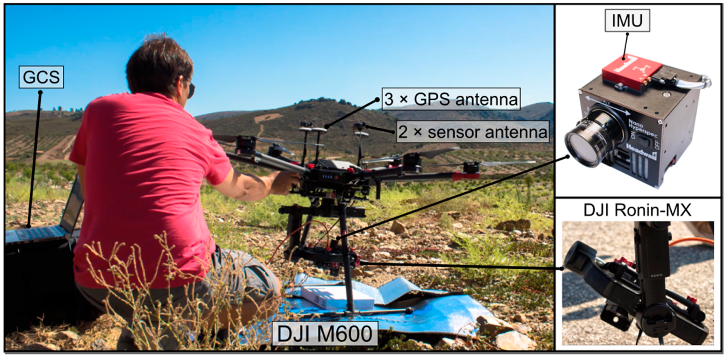
2.1.1. Nano-Hyperspec and DJI M600
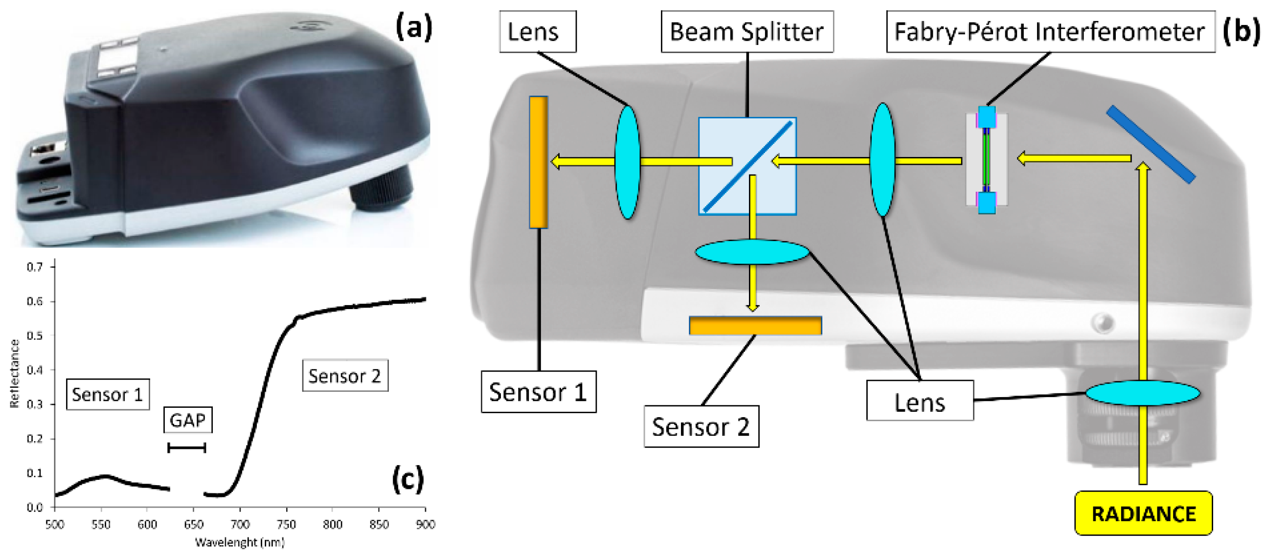
2.1.2. Senop Hyperspectral HSC-2 and DJI M600
2.2. Radiometric Correction
2.2.1. Nano-Hyperspec
2.2.2. Senop Hyperspectral HSC-2
2.3. Processing Workflow
2.3.1. Nano-Hyperspec
2.3.2. Senop HSC-2
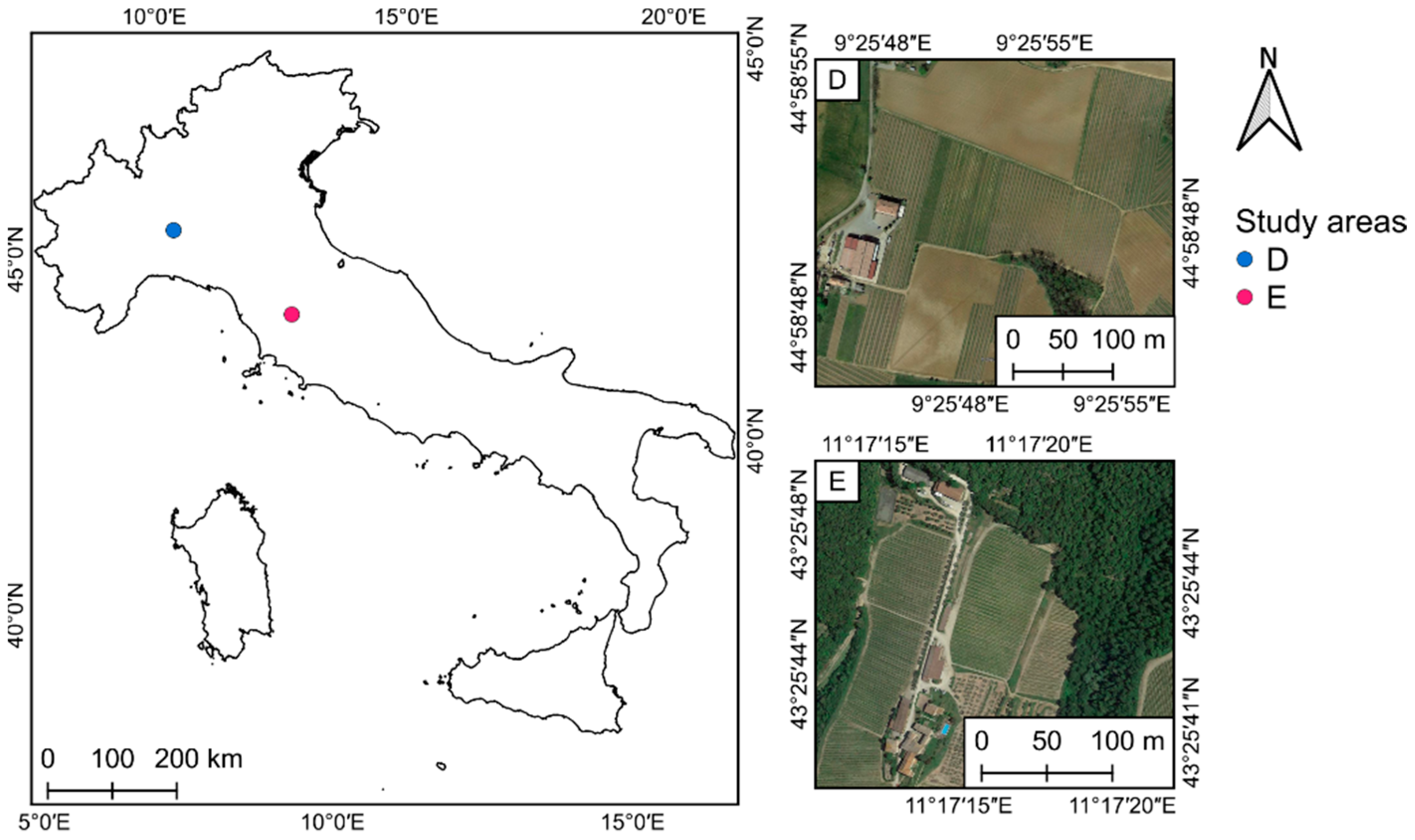
2.4. Study Areas
2.4.1. Nano-Hyperspec
2.4.2. Senop Hyperspectral Sensor HSC-2 Study Areas
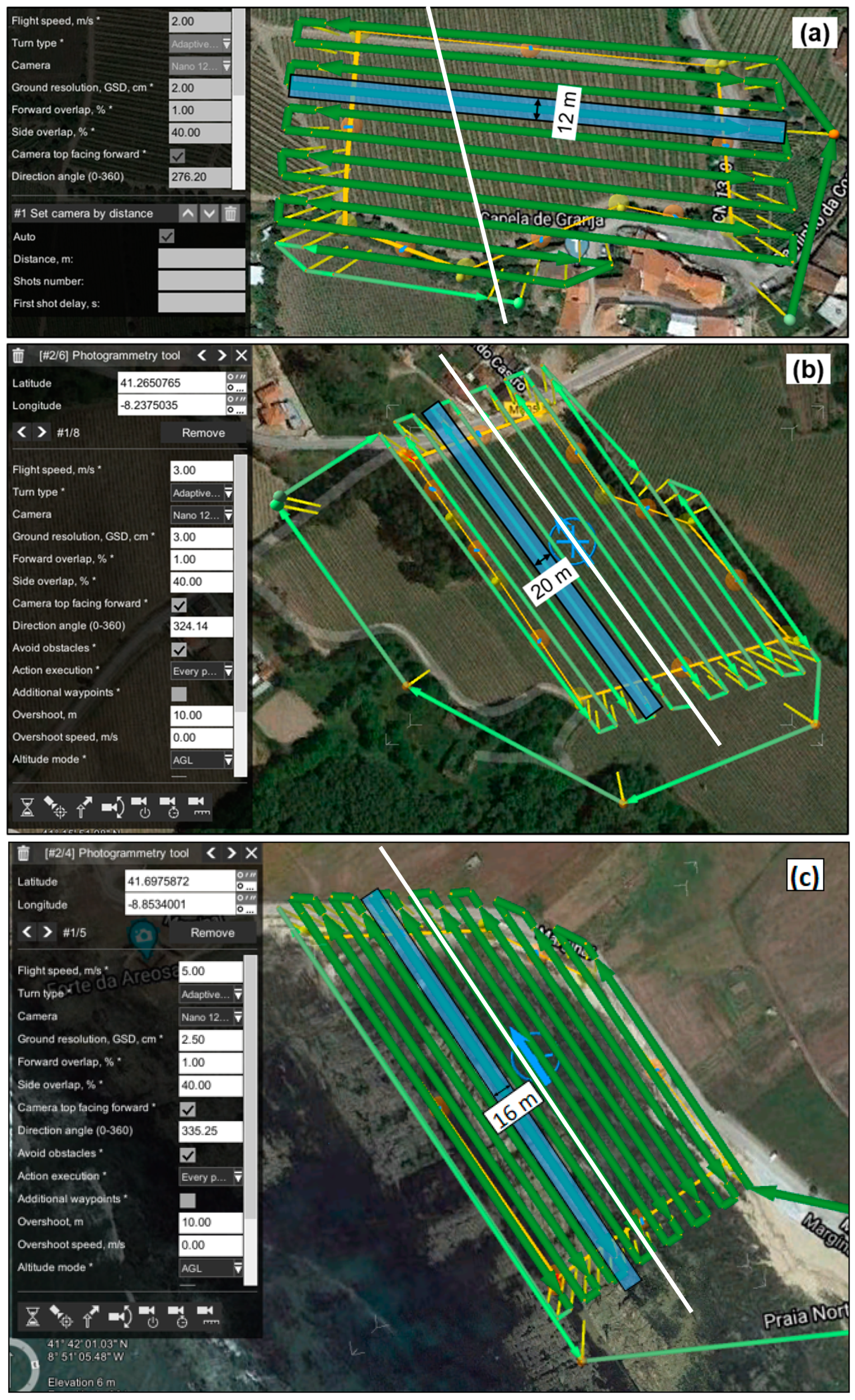
2.5. Data Collection
2.5.1. Nano-Hyperspec
2.5.2. Senop Hyperspectral HSC-2
3. Experimental Results
3.1. Nano-Hyperspec
3.2. Senop Hyperspectral HSC-2
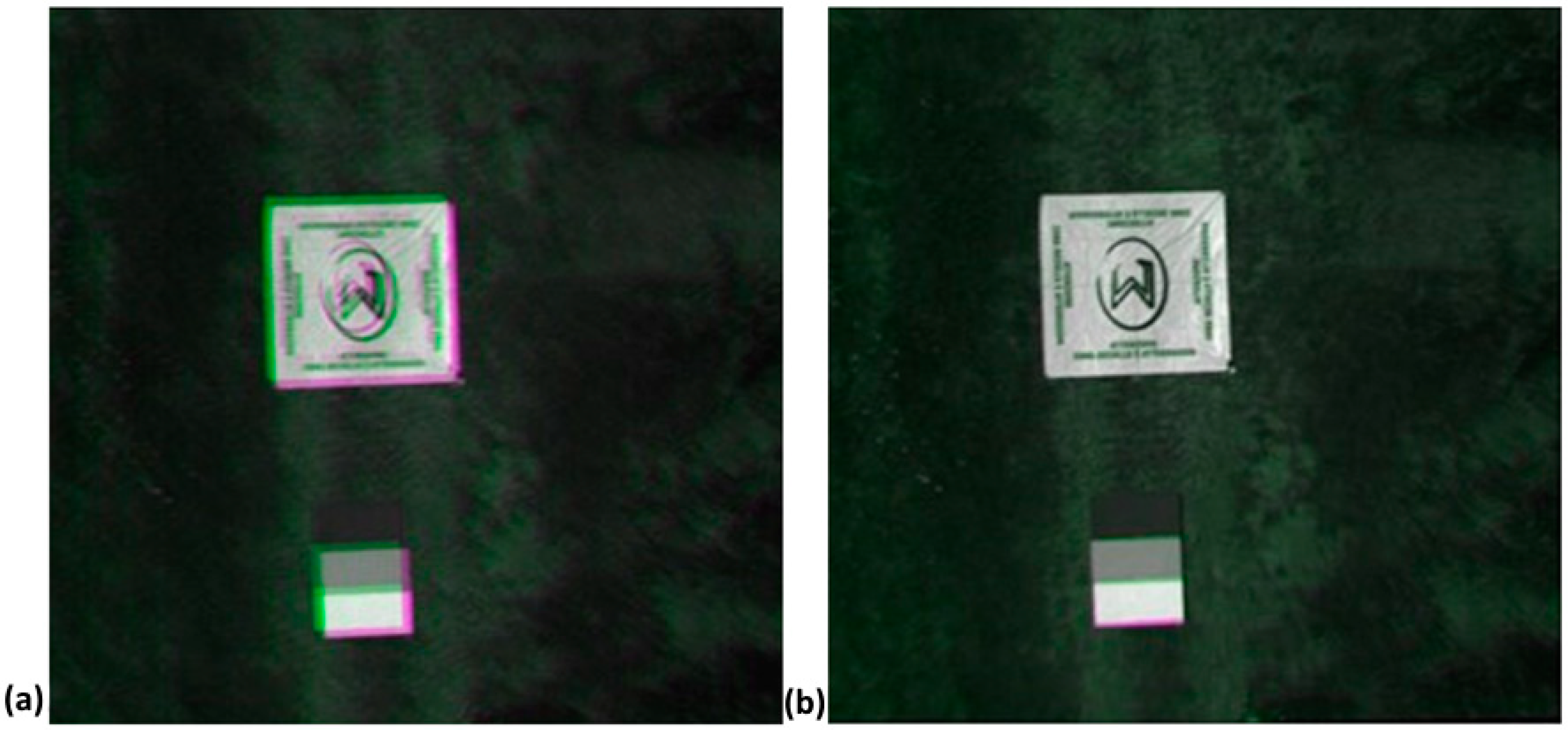
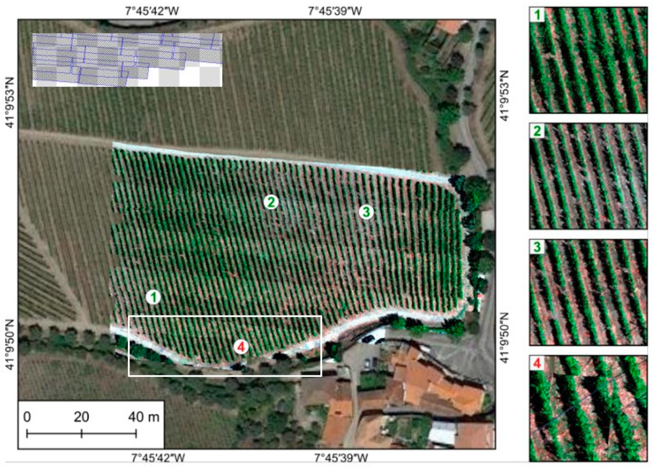
4. Qualitative Analysis
5. Conclusions
Author Contributions
Funding
Data Availability Statement
Conflicts of Interest
References
- Lu, B.; Dao, P.D.; Liu, J.; He, Y.; Shang, J. Recent Advances of Hyperspectral Imaging Technology and Applications in Agriculture. Remote Sens. 2020, 12, 2659. [Google Scholar] [CrossRef]
- Sabins, F.F. Remote Sensing for Mineral Exploration. Ore Geol. Rev. 1999, 14, 157–183. [Google Scholar] [CrossRef]
- Pascucci, S.; Pignatti, S.; Casa, R.; Darvishzadeh, R.; Huang, W. Special Issue “Hyperspectral Remote Sensing of Agriculture and Vegetation”. Remote Sens. 2020, 12, 3665. [Google Scholar] [CrossRef]
- Pastonchi, L.; Di Gennaro, S.F.; Toscano, P.; Matese, A. Comparison between Satellite and Ground Data with UAV-Based Information to Analyse Vineyard Spatio-Temporal Variability. Oeno One 2020, 54, 919–934. [Google Scholar]
- Pádua, L.; Marques, P.; Martins, L.; Sousa, A.; Peres, E.; Sousa, J.J. Monitoring of Chestnut Trees Using Machine Learning Techniques Applied to UAV-Based Multispectral Data. Remote Sens. 2020, 12, 3032. [Google Scholar] [CrossRef]
- Di Gennaro, S.F.; Dainelli, R.; Palliotti, A.; Toscano, P.; Matese, A. Sentinel-2 Validation for Spatial Variability Assessment in Overhead Trellis System Viticulture versus UAV and Agronomic Data. Remote Sens. 2019, 11, 2573. [Google Scholar] [CrossRef]
- Jiao, L.; Sun, W.; Yang, G.; Ren, G.; Liu, Y. A Hierarchical Classification Framework of Satellite Multispectral/Hyperspectral Images for Mapping Coastal Wetlands. Remote Sens. 2019, 11, 2238. [Google Scholar] [CrossRef]
- Pádua, L.; Antão-Geraldes, A.M.; Sousa, J.J.; Rodrigues, M.Â.; Oliveira, V.; Santos, D.; Miguens, M.F.P.; Castro, J.P. Water Hyacinth (Eichhornia Crassipes) Detection Using Coarse and High Resolution Multispectral Data. Drones 2022, 6, 47. [Google Scholar] [CrossRef]
- Song, A.; Choi, J.; Han, Y.; Kim, Y. Change Detection in Hyperspectral Images Using Recurrent 3D Fully Convolutional Networks. Remote Sens. 2018, 10, 1827. [Google Scholar] [CrossRef]
- Pádua, L.; Guimarães, N.; Adão, T.; Sousa, A.; Peres, E.; Sousa, J.J. Effectiveness of Sentinel-2 in Multi-Temporal Post-Fire Monitoring When Compared with UAV Imagery. ISPRS Int. J. Geo-Inf. 2020, 9, 225. [Google Scholar] [CrossRef]
- Luo, H.; Zhang, P.; Wang, J.; Wang, G.; Meng, F. Traffic Patrolling Routing Problem with Drones in an Urban Road System. Sensors 2019, 19, 5164. [Google Scholar] [CrossRef] [Green Version]
- Campbell, J.B.; Wynne, R.H. Introduction to Remote Sensing; Guilford Press: New York, NY, USA, 2011; ISBN 1-60918-177-8. [Google Scholar]
- Guimarães, N.; Pádua, L.; Marques, P.; Silva, N.; Peres, E.; Sousa, J.J. Forestry Remote Sensing from Unmanned Aerial Vehicles: A Review Focusing on the Data, Processing and Potentialities. Remote Sens. 2020, 12, 1046. [Google Scholar] [CrossRef]
- Pabian, F.V.; Renda, G.; Jungwirth, R.; Kim, L.K.; Wolfart, E.; Cojazzi, G.G.; Janssens, W.A. Commercial Satellite Imagery: An Evolving Tool in the Non-Proliferation Verification and Monitoring Toolkit. In Nuclear Non-proliferation and Arms Control Verification; Springer: Berlin/Heidelberg, Germany, 2020; pp. 351–371. [Google Scholar]
- Pádua, L.; Vanko, J.; Hruška, J.; Adão, T.; Sousa, J.J.; Peres, E.; Morais, R. UAS, Sensors, and Data Processing in Agroforestry: A Review towards Practical Applications. Int. J. Remote Sens. 2017, 38, 2349–2391. [Google Scholar] [CrossRef]
- Chen, H.; Miao, F.; Chen, Y.; Xiong, Y.; Chen, T. A Hyperspectral Image Classification Method Using Multifeature Vectors and Optimized KELM. IEEE J. Sel. Top. Appl. Earth Obs. Remote Sens. 2021, 14, 2781–2795. [Google Scholar] [CrossRef]
- PrecisionHawk Beyond the Edge-How Advanced Drones, Sensors, and Flight Operations Are Redefining the Limits of Remote Sensing. Available online: https://www.precisionhawk.com/sensors/advanced-sensors-and-data-collection/ (accessed on 27 September 2020).
- An, Z.; Wang, X.; Li, B.; Xiang, Z.; Zhang, B. Robust Visual Tracking for UAVs with Dynamic Feature Weight Selection. Appl. Intell. 2022, 1–14. [Google Scholar] [CrossRef]
- Matese, A.; Di Gennaro, S.F. Beyond the Traditional NDVI Index as a Key Factor to Mainstream the Use of UAV in Precision Viticulture. Sci. Rep. 2021, 11, 2721. [Google Scholar] [CrossRef]
- Pádua, L.; Adão, T.; Hruška, J.; Sousa, J.J.; Peres, E.; Morais, R.; Sousa, A. Very High Resolution Aerial Data to Support Multi-Temporal Precision Agriculture Information Management. Procedia Comput. Sci. 2017, 121, 407–414. [Google Scholar] [CrossRef]
- Goetz, A.F.; Vane, G.; Solomon, J.E.; Rock, B.N. Imaging Spectrometry for Earth Remote Sensing. Science 1985, 228, 1147–1153. [Google Scholar] [CrossRef] [PubMed]
- Ball, D.W. The Basics of Spectroscopy; Spie Press: Bellingham, WA, USA, 2001; Volume 49, ISBN 0-8194-4104-X. [Google Scholar]
- Grahn, H.; Geladi, P. Techniques and Applications of Hyperspectral Image Analysis; John Wiley & Sons: Hoboken, NJ, USA, 2007; ISBN 0-470-01087-8. [Google Scholar]
- Adão, T.; Hruška, J.; Pádua, L.; Bessa, J.; Peres, E.; Morais, R.; Sousa, J.J. Hyperspectral Imaging: A Review on UAV-Based Sensors, Data Processing and Applications for Agriculture and Forestry. Remote Sens. 2017, 9, 1110. [Google Scholar] [CrossRef]
- Jurado, J.M.; López, A.; Pádua, L.; Sousa, J.J. Remote Sensing Image Fusion on 3D Scenarios: A Review of Applications for Agriculture and Forestry. Int. J. Appl. Earth Obs. Geoinf. 2022, 112, 102856. [Google Scholar] [CrossRef]
- Kerekes, J.P.; Schott, J.R. Hyperspectral Imaging Systems. Hyperspectral Data Exploit. Theory Appl. 2007, 1, 19–45. [Google Scholar]
- Aasen, H.; Honkavaara, E.; Lucieer, A.; Zarco-Tejada, P.J. Quantitative Remote Sensing at Ultra-High Resolution with UAV Spectroscopy: A Review of Sensor Technology, Measurement Procedures, and Data Correction Workflows. Remote Sens. 2018, 10, 1091. [Google Scholar] [CrossRef] [Green Version]
- Oliveira, R.A.; Tommaselli, A.M.; Honkavaara, E. Generating a Hyperspectral Digital Surface Model Using a Hyperspectral 2D Frame Camera. ISPRS J. Photogramm. Remote Sens. 2019, 147, 345–360. [Google Scholar] [CrossRef]
- Tommaselli, A.M.; Oliveira, R.A.; Nagai, L.Y.; Imai, N.N.; Miyoshi, G.T.; Honkavaara, E.; Hakala, T. Assessment of Bands Coregistration of a Light-Weight Spectral Frame Camera for UAV. GeoUAV-ISPRS Geospat. Week 2015, 192. [Google Scholar]
- Honkavaara, E.; Saari, H.; Kaivosoja, J.; Pölönen, I.; Hakala, T.; Litkey, P.; Mäkynen, J.; Pesonen, L. Processing and Assessment of Spectrometric, Stereoscopic Imagery Collected Using a Lightweight UAV Spectral Camera for Precision Agriculture. Remote Sens. 2013, 5, 5006–5039. [Google Scholar] [CrossRef]
- Jakob, S.; Zimmermann, R.; Gloaguen, R. The Need for Accurate Geometric and Radiometric Corrections of Drone-Borne Hyperspectral Data for Mineral Exploration: Mephysto—A Toolbox for Pre-Processing Drone-Borne Hyperspectral Data. Remote Sens. 2017, 9, 88. [Google Scholar] [CrossRef]
- Booysen, R.; Jackisch, R.; Lorenz, S.; Zimmermann, R.; Kirsch, M.; Nex, P.A.; Gloaguen, R. Detection of REEs with Lightweight UAV-Based Hyperspectral Imaging. Sci. Rep. 2020, 10, 17450. [Google Scholar] [CrossRef]
- Geipel, J.; Bakken, A.K.; Jørgensen, M.; Korsaeth, A. Forage Yield and Quality Estimation by Means of UAV and Hyperspectral Imaging. Precis. Agric. 2021, 22, 1437–1463. [Google Scholar] [CrossRef]
- Chancia, R.; Bates, T.; Heuvel, J.V.; van Aardt, J. Assessing Grapevine Nutrient Status from Unmanned Aerial System (UAS) Hyperspectral Imagery. Remote Sens. 2021, 13, 4489. [Google Scholar] [CrossRef]
- Červená, L.; Pinlová, G.; Lhotáková, Z.; Neuwirthová, E.; Kupková, L.; Potůčková, M.; Lysák, J.; Campbell, P.; Albrechtová, J. Determination of Chlorophyll Content in Selected Grass Communities of KRKONOŠE Mts. Tundra Based on Laboratory Spectroscopy and Aerial Hyperspectral data. In Proceedings of the International Archives of the Photogrammetry, Remote Sensing and Spatial Information Sciences, Nice, France, 6–11 June 2022; Copernicus GmbH: Göttingen, Germany; Volume XLIII-B3-2022, pp. 381–388. [Google Scholar]
- Ge, X.; Ding, J.; Jin, X.; Wang, J.; Chen, X.; Li, X.; Liu, J.; Xie, B. Estimating Agricultural Soil Moisture Content through UAV-Based Hyperspectral Images in the Arid Region. Remote Sens. 2021, 13, 1562. [Google Scholar] [CrossRef]
- Vanegas, F.; Bratanov, D.; Powell, K.; Weiss, J.; Gonzalez, F. A Novel Methodology for Improving Plant Pest Surveillance in Vineyards and Crops Using UAV-Based Hyperspectral and Spatial Data. Sensors 2018, 18, 260. [Google Scholar] [CrossRef] [PubMed]
- Fan, J.; Zhou, J.; Wang, B.; de Leon, N.; Kaeppler, S.M.; Lima, D.C.; Zhang, Z. Estimation of Maize Yield and Flowering Time Using Multi-Temporal UAV-Based Hyperspectral Data. Remote Sens. 2022, 14, 3052. [Google Scholar] [CrossRef]
- Cao, J.; Liu, K.; Zhuo, L.; Liu, L.; Zhu, Y.; Peng, L. Combining UAV-Based Hyperspectral and LiDAR Data for Mangrove Species Classification Using the Rotation Forest Algorithm. Int. J. Appl. Earth Obs. Geoinf. 2021, 102, 102414. [Google Scholar] [CrossRef]
- Rossiter, T.; Furey, T.; McCarthy, T.; Stengel, D.B. UAV-Mounted Hyperspectral Mapping of Intertidal Macroalgae. Estuar. Coast. Shelf Sci. 2020, 242, 106789. [Google Scholar] [CrossRef]
- Di Gennaro, S.F.; Toscano, P.; Gatti, M.; Poni, S.; Berton, A.; Matese, A. Spectral Comparison of UAV-Based Hyper and Multispectral Cameras for Precision Viticulture. Remote Sens. 2022, 14, 449. [Google Scholar] [CrossRef]
- Matese, A.; Di Gennaro, S.F.; Orlandi, G.; Gatti, M.; Poni, S. Assessing Grapevine Biophysical Parameters From Unmanned Aerial Vehicles Hyperspectral Imagery. Front. Plant Sci. 2022, 13, 8722. [Google Scholar] [CrossRef]
- Moriya, É.A.S.; Imai, N.N.; Tommaselli, A.M.G.; Berveglieri, A.; Santos, G.H.; Soares, M.A.; Marino, M.; Reis, T.T. Detection and Mapping of Trees Infected with Citrus Gummosis Using UAV Hyperspectral Data. Comput. Electron. Agric. 2021, 188, 106298. [Google Scholar] [CrossRef]
- Abenina, M.I.A.; Maja, J.M.; Cutulle, M.; Melgar, J.C.; Liu, H. Prediction of Potassium in Peach Leaves Using Hyperspectral Imaging and Multivariate Analysis. AgriEngineering 2022, 4, 400–413. [Google Scholar] [CrossRef]
- da Silva, A.R.; Demarchi, L.; Sikorska, D.; Sikorski, P.; Archiciński, P.; Jóźwiak, J.; Chormański, J. Multi-Source Remote Sensing Recognition of Plant Communities at the Reach Scale of the Vistula River, Poland. Ecol. Indic. 2022, 142, 109160. [Google Scholar] [CrossRef]
- Näsi, R.; Viljanen, N.; Kaivosoja, J.; Alhonoja, K.; Hakala, T.; Markelin, L.; Honkavaara, E. Estimating Biomass and Nitrogen Amount of Barley and Grass Using UAV and Aircraft Based Spectral and Photogrammetric 3D Features. Remote Sens. 2018, 10, 1082. [Google Scholar] [CrossRef]
- Tao, H.; Feng, H.; Xu, L.; Miao, M.; Yang, G.; Yang, X.; Fan, L. Estimation of the Yield and Plant Height of Winter Wheat Using UAV-Based Hyperspectral Images. Sensors 2020, 20, 1231. [Google Scholar] [CrossRef] [PubMed]
- Yue, J.; Feng, H.; Jin, X.; Yuan, H.; Li, Z.; Zhou, C.; Yang, G.; Tian, Q. A Comparison of Crop Parameters Estimation Using Images from UAV-Mounted Snapshot Hyperspectral Sensor and High-Definition Digital Camera. Remote Sens. 2018, 10, 1138. [Google Scholar] [CrossRef]
- Shin, J.-I.; Cho, Y.-M.; Lim, P.-C.; Lee, H.-M.; Ahn, H.-Y.; Park, C.-W.; Kim, T. Relative Radiometric Calibration Using Tie Points and Optimal Path Selection for UAV Images. Remote Sens. 2020, 12, 1726. [Google Scholar] [CrossRef]
- Guo, Y.; Senthilnath, J.; Wu, W.; Zhang, X.; Zeng, Z.; Huang, H. Radiometric Calibration for Multispectral Camera of Different Imaging Conditions Mounted on a UAV Platform. Sustainability 2019, 11, 978. [Google Scholar] [CrossRef]
- Xu, K.; Gong, Y.; Fang, S.; Wang, K.; Lin, Z.; Wang, F. Radiometric Calibration of UAV Remote Sensing Image with Spectral Angle Constraint. Remote Sens. 2019, 11, 1291. [Google Scholar] [CrossRef]
- Yuan, H.; Yang, G.; Li, C.; Wang, Y.; Liu, J.; Yu, H.; Feng, H.; Xu, B.; Zhao, X.; Yang, X. Retrieving Soybean Leaf Area Index from Unmanned Aerial Vehicle Hyperspectral Remote Sensing: Analysis of RF, ANN, and SVM Regression Models. Remote Sens. 2017, 9, 309. [Google Scholar] [CrossRef]
- Kay, L.; Shepherd, R. Instrument Function for Ebert and Czerny-Turner Scanning Monochromators Used with Long Straight Slits. J. Phys. E Sci. Instrum. 1983, 16, 295. [Google Scholar] [CrossRef]
- Aasen, H.; Burkart, A.; Bolten, A.; Bareth, G. Generating 3D Hyperspectral Information with Lightweight UAV Snapshot Cameras for Vegetation Monitoring: From Camera Calibration to Quality Assurance. ISPRS J. Photogramm. Remote Sens. 2015, 108, 245–259. [Google Scholar] [CrossRef]
- Liu, Y.; Wang, T.; Ma, L.; Wang, N. Spectral Calibration of Hyperspectral Data Observed from a Hyperspectrometer Loaded on an Unmanned Aerial Vehicle Platform. IEEE J. Sel. Top. Appl. Earth Obs. Remote Sens. 2014, 7, 2630–2638. [Google Scholar] [CrossRef]
- Yang, G.; Li, C.; Wang, Y.; Yuan, H.; Feng, H.; Xu, B.; Yang, X. The DOM Generation and Precise Radiometric Calibration of a UAV-Mounted Miniature Snapshot Hyperspectral Imager. Remote Sens. 2017, 9, 642. [Google Scholar] [CrossRef]
- Barreto, M.A.P.; Johansen, K.; Angel, Y.; McCabe, M.F. Radiometric Assessment of a UAV-Based Push-Broom Hyperspectral Camera. Sensors 2019, 19, 4699. [Google Scholar] [CrossRef] [PubMed]
- Wang, C.; Myint, S.W. A Simplified Empirical Line Method of Radiometric Calibration for Small Unmanned Aircraft Systems-Based Remote Sensing. IEEE J. Sel. Top. Appl. Earth Obs. Remote Sens. 2015, 8, 1876–1885. [Google Scholar] [CrossRef]
- Gómez-Chova, L.; Alonso, L.; Guanter, L.; Camps-Valls, G.; Calpe, J.; Moreno, J. Correction of Systematic Spatial Noise in Push-Broom Hyperspectral Sensors: Application to CHRIS/PROBA Images. Appl. Opt. 2008, 47, F46–F60. [Google Scholar] [CrossRef] [PubMed] [Green Version]
- Smith, G.M.; Milton, E.J. The Use of the Empirical Line Method to Calibrate Remotely Sensed Data to Reflectance. Int. J. Remote Sens. 1999, 20, 2653–2662. [Google Scholar] [CrossRef]
- Herrero-Huerta, M.; Hernández-López, D.; Rodriguez-Gonzalvez, P.; González-Aguilera, D.; González-Piqueras, J. Vicarious Radiometric Calibration of a Multispectral Sensor from an Aerial Trike Applied to Precision Agriculture. Comput. Electron. Agric. 2014, 108, 28–38. [Google Scholar] [CrossRef]
- UgCS Ground Station Software | UgCS PC Mission Planning. Available online: https://www.ugcs.com/ (accessed on 7 July 2022).
- Zarco-Tejada, P.J.; Diaz-Varela, R.; Angileri, V.; Loudjani, P. Tree Height Quantification Using very High Resolution Imagery Acquired from an Unmanned Aerial Vehicle (UAV) and Automatic 3D Photo-Reconstruction Methods. Eur. J. Agron. 2014, 55, 89–99. [Google Scholar] [CrossRef]
- Harwin, S.; Lucieer, A.; Osborn, J. The Impact of the Calibration Method on the Accuracy of Point Clouds Derived Using Unmanned Aerial Vehicle Multi-View Stereopsis. Remote Sens. 2015, 7, 11933–11953. [Google Scholar] [CrossRef] [Green Version]


| Manufacturer | Sensor | Spectral Range (nm) | No. of Bands | Spectral Resolution (nm) | Spatial Resolution (px) | Acquisition Mode | Weight (kg) |
|---|---|---|---|---|---|---|---|
| BaySpec | OCI-UAV-1000 | — | 100 | <5 | 2048 | Push-broom | 0.272 |
| Brandywine Photonics | CHAI S-640 | — | 260 | 2.5–5 | 640 × 512 | Push-broom | 5 |
| CHAI V-640 | — | 256 | 5–10 | 640 × 512 | Push-broom | 0.48 | |
| Cubert GmbH | S 185—FIREFLEYE SE | 450–950 355–750 | 125 | 4 | 50 × 50 | Snapshot | 0.49 |
| S 485—FIREFLEYE XL | 450–950 550–1000 | 125 | 4.5 | 70 × 70 | Snapshot | 1.2 | |
| Q 285—FIREFLEYE QE | 450–950 | 125 | 4 | 50 × 50 | Snapshot | 3 | |
| Headwall Photonics Inc. | Nano HyperSpec | 400–1000 | 272–775 | 6 | 640 | Push-broom | 1.2 |
| Micro Hyperspec VNIR | 380-1000 | 837–923 | 2.5 | 1004 1600 | Push-broom | ~3.9 | |
| HySpex | VNIR-1024 | 400–1000 | 108 | 5.4 | 1024 | Push-broom | 4 |
| Mjolnir V-1240 | 400–1000 | 200 | 3 | 1240 | Push-broom | 4.2 | |
| HySpex SWIR-384 | 1000–2500 | 288 | 5.45 | 384 | Push-broom | 5.7 | |
| NovaSol | vis-NIR microHSI | 400–800 | 120 | 3.3 | 680 | Push-broom | ~0.45 |
| 400–1000 | 180 | ||||||
| 380–880 | 150 | ||||||
| Alpha-vis micro HSI | 400–800 | 40 | 10 | 1280 | Push-broom | ~2.1 | |
| 350–1000 | 60 | ||||||
| SWIR 640 microHSI | 850–1700 | 170 | 5 | 640 | Push-broom | 3.5 | |
| 600–1700 | 200 | ||||||
| Alpha-SWIR microHSI | 900–1700 | 160 | 5 | 640 | Push-broom | 1.2 | |
| Extra-SWIR microHSI | 964–2500 | 256 | 6 | 320 | Push-broom | 2.6 | |
| PhotonFocus | MV1-D2048x1088-HS05-96-G2 | 470–900 | 150 | 10–12 | 2048 × 1088 | Push-broom | 0.265 |
| Quest Innovations | Hyperea 660 C1 | 400–1000 | 660 | - | 1024 | Push-broom | 1.44 |
| Resonon | Pika L | 400–1000 | 281 | 2.1 | 900 | Push-broom | 0.6 |
| Pika CX2 | 400–1000 | 447 | 1.3 | 1600 | Push-broom | 2.2 | |
| Pika NIR | 900–1700 | 164 | 4.9 | 320 | Push-broom | 2.7 | |
| Pika NUV | 350–800 | 196 | 2.3 | 1600 | Push-broom | 2.1 | |
| SENOP | VIS-VNIR Snapshot | 400–900 | 380 | 10 | 1010 × 1010 | Snapshot | 0.72 |
| SPECIM | SPECIM FX10 | 400–1000 | 224 | 5.5 | 1024 | Push-broom | 1.26 |
| SPECIM FX17 | 900–1700 | 224 | 8 | 640 | Push-broom | 1.7 | |
| Surface Optics Corp. | SOC710-GX | 400–1000 | 120 | 4.2 | 640 | Push-broom | 1.25 |
| XIMEA | MQ022HG-IM-LS100-NIR | 600–975 | 100+ | 4 | 2048 × 8 | Push-broom | 0.032 |
| MQ022HG-IM-LS150-VISNIR | 470–900 | 150+ | 3 | 2048 × 5 | Push-broom | 0.3 |
| Wavelength Range (nm) | 400–1000 | Camera Technology | CMOS |
| Spatial bands | 640 | Bit depth | 12-bit |
| Spectral bands | 272 | Max Frame Rate (Hz) | 350 |
| Dispersion/Pixel (nm/pixel) | 2.2 | Detector pixel pitch (µm) | 7.4 |
| FWHM Slit Image (nm) | 6 | Max Power (W) | 13 |
| f/# | 2.5 | Storage capacity (GB) | 480 |
| Entrance Slit width (µm) | 20 | Operating Temperature (ºC) | 0–50 |
| Weight without lens (kg) | 0.5 | GPS | Integrated |
| Optics | F#3.28 | Image Frame Size (Pixels) | 1024 × 1024 |
| FOV | 36.8° | Frame rate (single image or video) | 12-bit frame: max 74 f/s 10-bit image: max 149 f/s |
| Focus distance | 30 cm to ∞ | Wavelength area (nm) | 500–900 (up to 1000 spectral bands) |
| Exposure time | can be set freely | Spectral FWHM bandwidth | Narrow < 15 nm, Normal < 20 nm, Wide < 25 nm |
| Integrated IMU | Accuracy typically 1° | Storage | 1TB (Internal Hard Drive) |
| Size (mm) | 199.5 × 130.9 × 97.2 | GPS | Integrated GPS |
| Weight (g) | 990 | Antenna | Internal antenna for GPS |
| Study Area | Area (ha) | Slope (%) | Spacing (m) Inter-Row × Intra-Row |
|---|---|---|---|
| Vallado | 1.5 | 20 | 2.2 × 1.3 |
| Chianti | 1.2 | 17 | 2.2 × 0.75 |
| Lousada | 2 | flat | 2.8 × 1.75 |
| Piacenza | 1 | flat | 2.4 × 1.0 |
| Area | No DEM | SRTM DEM | UAV DEM |
|---|---|---|---|
| Vallado |  |  |  |
| Lousada |  |  |  |
| Viana |  |  |  |
| Study Area | Parameters | Processing Time (Hours) | Mosaic Size (Gbyte) | |||
|---|---|---|---|---|---|---|
| Pitch (Deg) | Roll (Deg) | Yaw (Deg) | Alt. Offset (m) | |||
| Vallado | 0 | 0 | 0 | −125 | 8 | ~60 |
| 1.8 | 0 | −2 | ||||
| 0 | 0 | 0 | ||||
| −3 | 4 | 0 | ||||
| −0.5 | 0 | 2 | ||||
| 0 | −2 | 0 | ||||
| 1 | 0 | −1 | ||||
| 1 | 2 | 0 | ||||
| 0 | 0 | 1 | ||||
| 1 | −1 | −1 | ||||
| Lousada | −1 | −1 | 0 | −170 | 7 | ~65 |
| 0 | −2 | 0 | ||||
| −1 | −2.3 | 0 | ||||
| 0 | −2 | 0 | ||||
| −1.2 | −1.5 | 0 | ||||
| 0 | −2 | 0 | ||||
| −1.2 | −1.5 | 0 | ||||
| 0 | −2 | 0 | ||||
| −1.2 | −1.5 | 0 | ||||
| 0 | −2 | 0 | ||||
| Viana | 0 | 0 | 0 | −60 | 2 | ~80 |
| Study Area | Pixel Res. (cm) | Frame Size of Each Band | No. of Frames | No. of Bands | Mosaic Size (Gbyte) | Pre-Processing Time (h) | Mosaic Processing Time per Band |
|---|---|---|---|---|---|---|---|
| Piacenza | 2 | 8 MB | 215 | 50 | 8.5 | 2 | 12 min |
| Chianti | 2 | 8 MB | 540 | 50 | 11.5 | 2.5 | 15 min |
| Sensor Type | Push-Broom | Snapshot |
| Acquisition design | Scanner | Optical |
| No. of bands | ++ | +++ * |
| Spectral coverage | ++ | ++ |
| Processing time | +++ | ++ |
| Bands co-registration | +++ | + |
| Processing complexity | + (multiple swaths) +++ (single swath) | + |
| Flight planning | +++ | ++ |
| Limitations | -Spatial distortions -Data alignment with other sensors -Orthorectification in topographically complex areas | -Radiometric calibration -Bands co-registration -GCPs dependent -Complex field operation |
| Advantages | Bands co-registration | Simple individual bands processing (compared to RGB) |
Publisher’s Note: MDPI stays neutral with regard to jurisdictional claims in published maps and institutional affiliations. |
© 2022 by the authors. Licensee MDPI, Basel, Switzerland. This article is an open access article distributed under the terms and conditions of the Creative Commons Attribution (CC BY) license (https://creativecommons.org/licenses/by/4.0/).
Share and Cite
Sousa, J.J.; Toscano, P.; Matese, A.; Di Gennaro, S.F.; Berton, A.; Gatti, M.; Poni, S.; Pádua, L.; Hruška, J.; Morais, R.; et al. UAV-Based Hyperspectral Monitoring Using Push-Broom and Snapshot Sensors: A Multisite Assessment for Precision Viticulture Applications. Sensors 2022, 22, 6574. https://doi.org/10.3390/s22176574
Sousa JJ, Toscano P, Matese A, Di Gennaro SF, Berton A, Gatti M, Poni S, Pádua L, Hruška J, Morais R, et al. UAV-Based Hyperspectral Monitoring Using Push-Broom and Snapshot Sensors: A Multisite Assessment for Precision Viticulture Applications. Sensors. 2022; 22(17):6574. https://doi.org/10.3390/s22176574
Chicago/Turabian StyleSousa, Joaquim J., Piero Toscano, Alessandro Matese, Salvatore Filippo Di Gennaro, Andrea Berton, Matteo Gatti, Stefano Poni, Luís Pádua, Jonáš Hruška, Raul Morais, and et al. 2022. "UAV-Based Hyperspectral Monitoring Using Push-Broom and Snapshot Sensors: A Multisite Assessment for Precision Viticulture Applications" Sensors 22, no. 17: 6574. https://doi.org/10.3390/s22176574