
Rapid Seismic Evaluation of Continuous Girder Bridges with Localized Plastic Hinges

Abstract
:1. Introduction
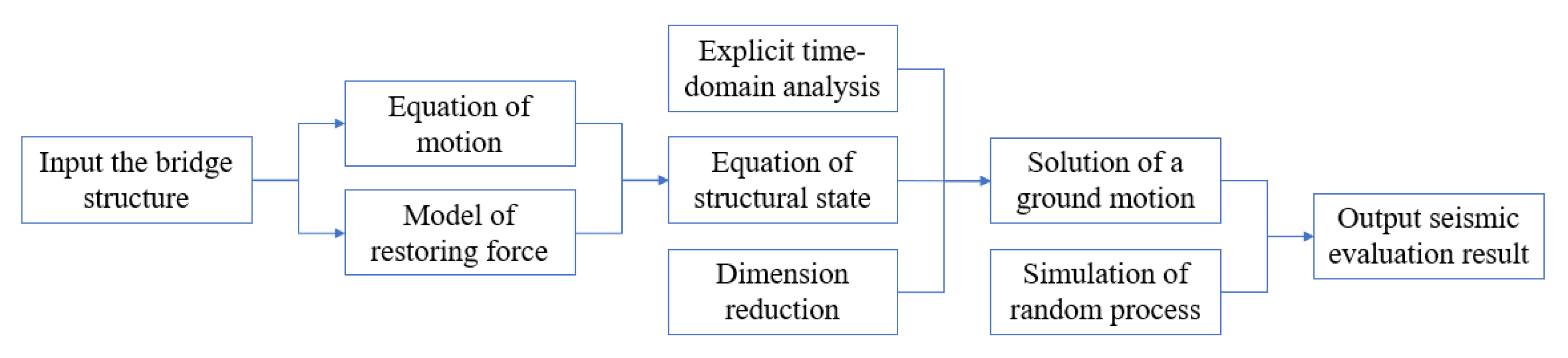
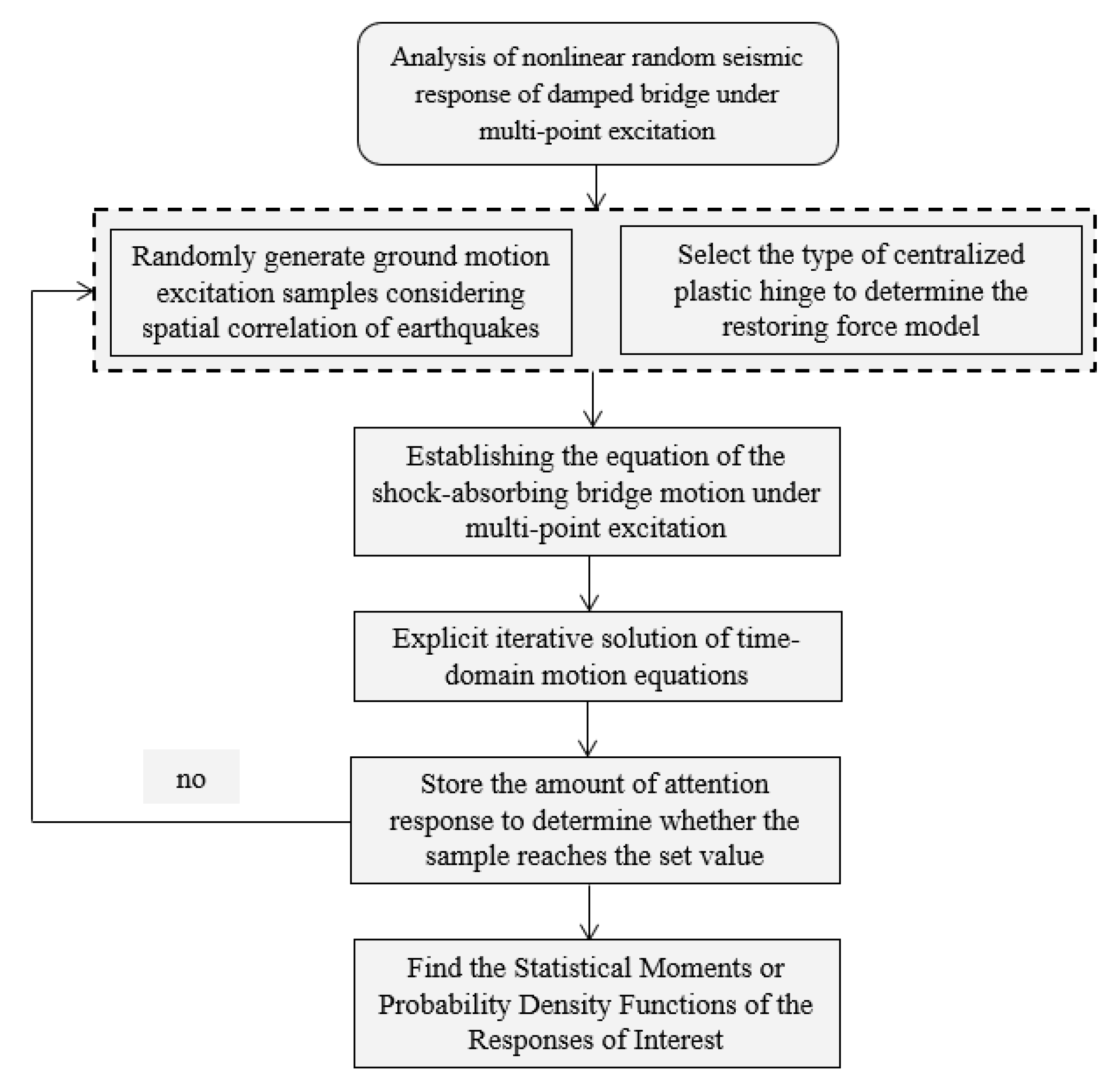
2. Methodology
2.1. Equation of Motion
2.2. Restoring Force Model of Plastic Hinges
2.3. Equation of State for Explicit Time-Domain Analysis
2.4. Dimension Reduction
2.5. Simulation of Random Processes
3. Case Study
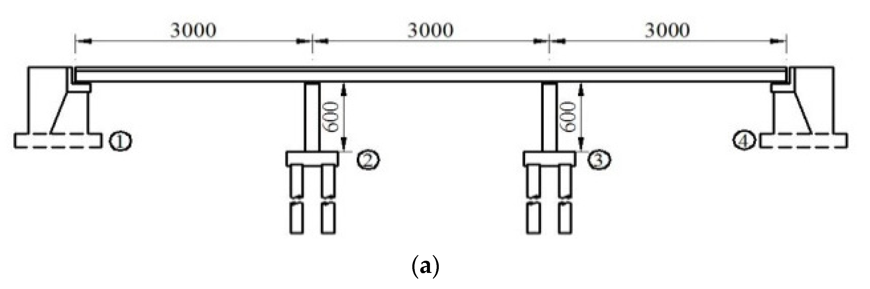
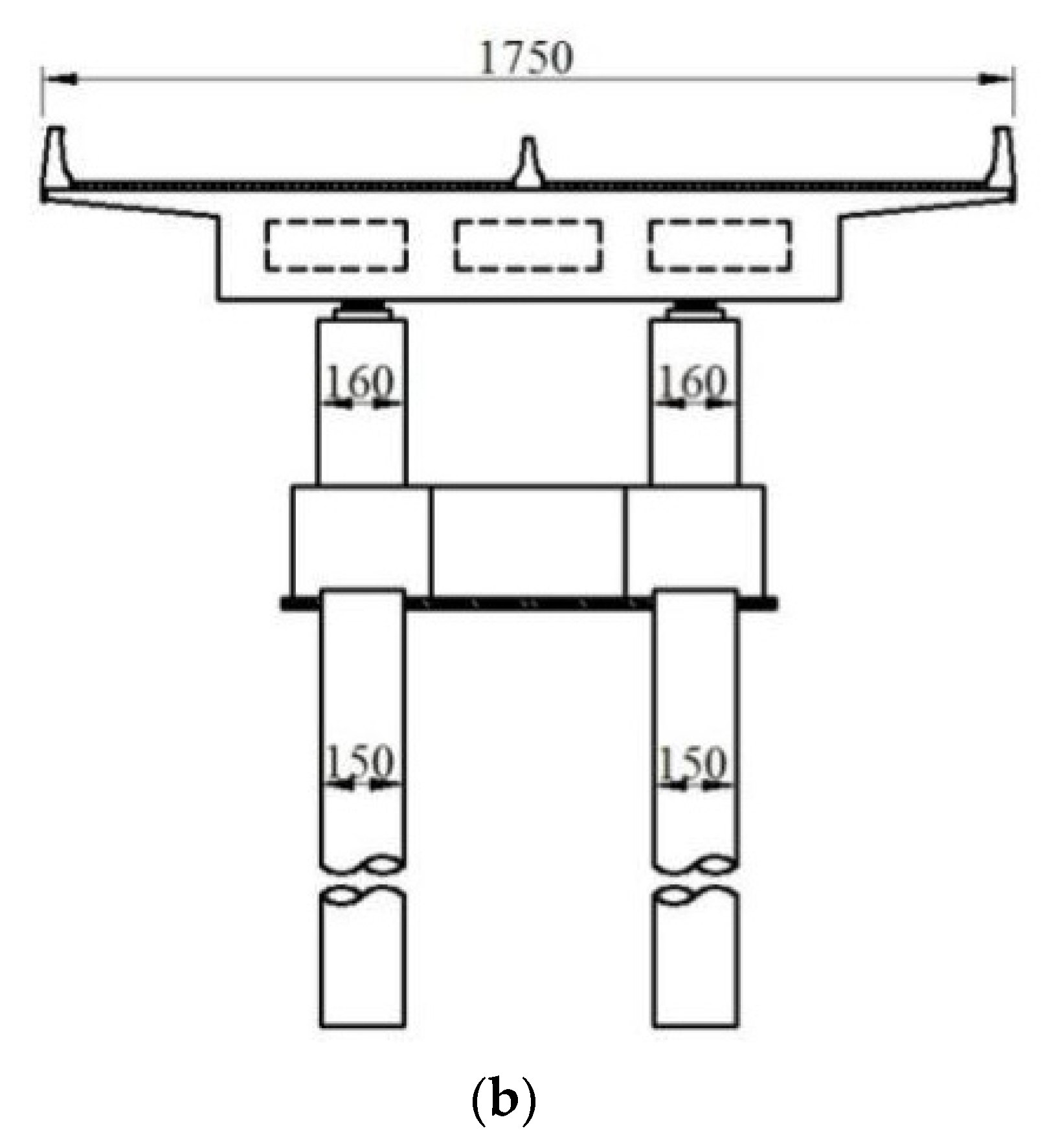
3.1. Bridge Description
3.2. Power Spectrum Model of Ground Motions
3.3. Spatially Varying Excitation
3.4. Results and Discussions
4. Conclusions
- (1)
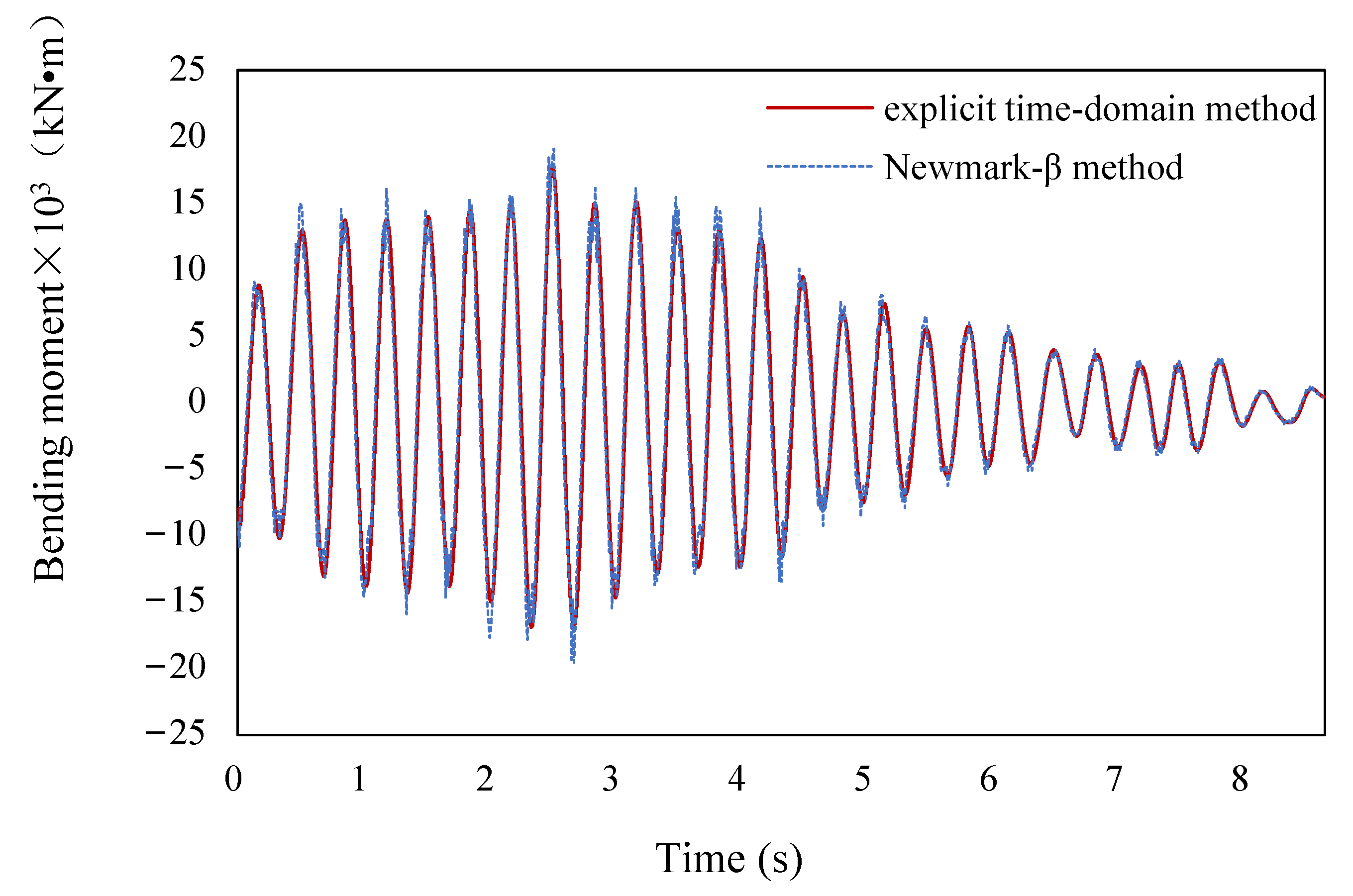
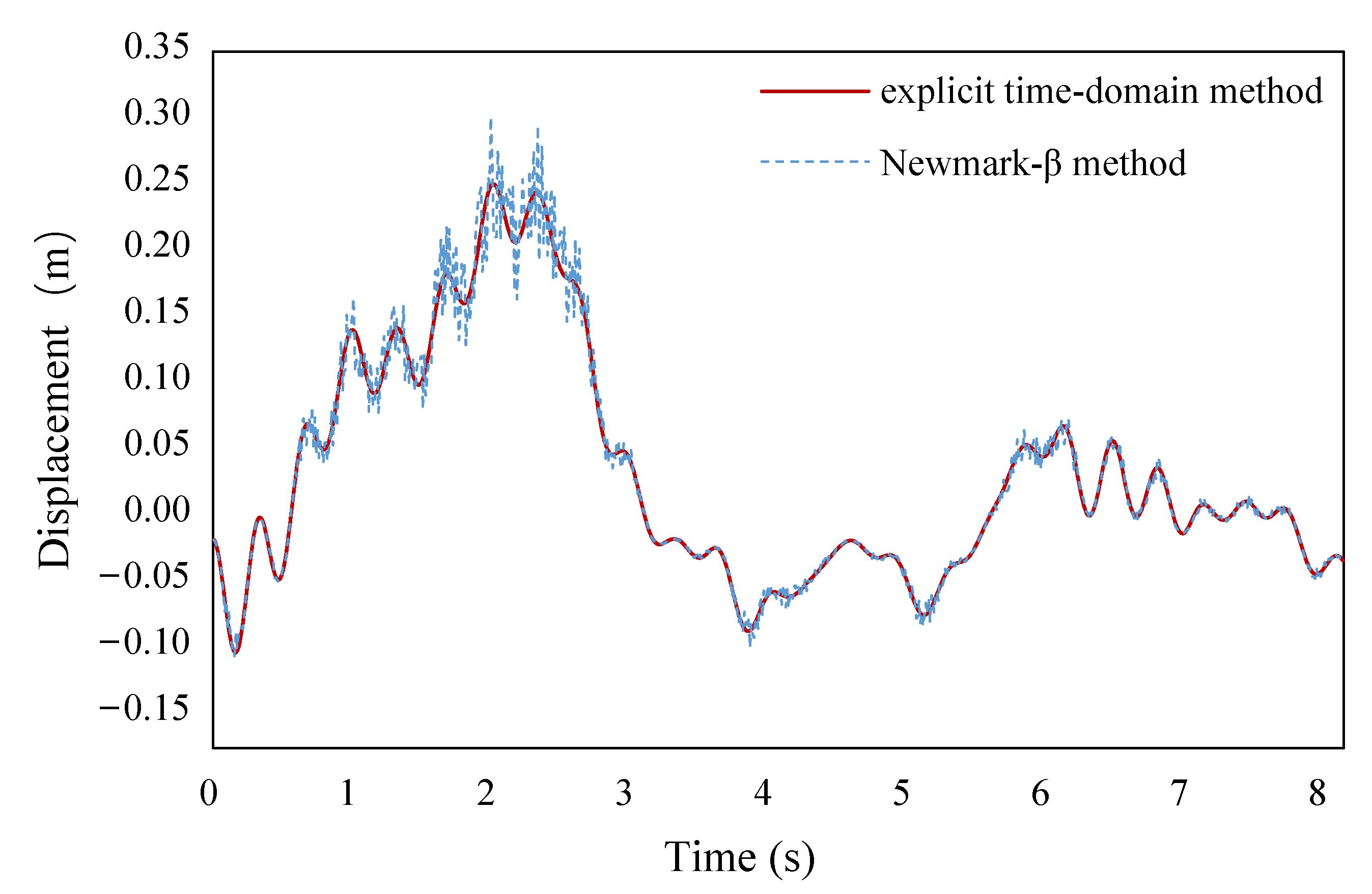
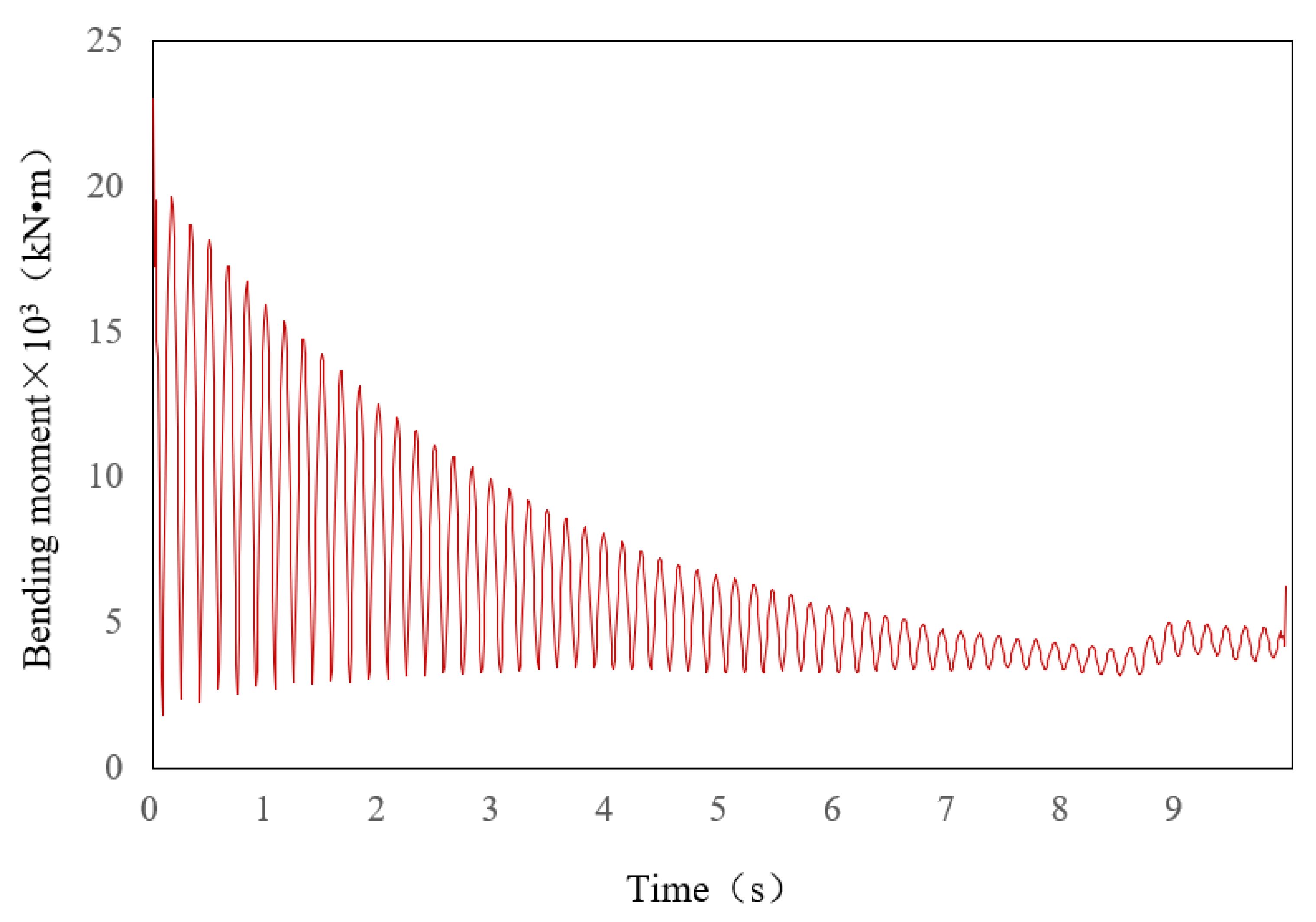
- The proposed approach is accurate. The seismic performance evaluation of continuous girder bridges mainly focuses on the seismic performance of piers with fixed hinges. The seismic performance evaluation index is mainly based on pier top section displacement, pier bottom section bending moment–curvature, etc. The time history diagrams of pier top section displacement and the pier bottom section bending moment are consistent with the response characteristics of general dynamic problems, so the accuracy of the method can be known.
- (2)
- The proposed approach significantly improves the computational efficiency. Once determined in the first round of analysis, the coefficient matrices in the equations are preserved throughout the analysis. Preservation of the coefficient matrices simplifies the computation process, thus improving computational efficiency. Such improvement is particularly relevant for seismic evaluation because the evaluation involves stochastic processes and requires repeated computations. Compared with the conventional nonlinear time history dynamic analysis performed, the computation time of the proposed approach is only 5%, and the maximum error of the displacement of the pier top section and the bending moment of the pier bottom section is within 10%. The high efficiency of the proposed approach is achieved by the combination of multiple techniques such as explicit time domain analysis using the state equations, the precision integration method, and the dimension reduction method.
- (3)
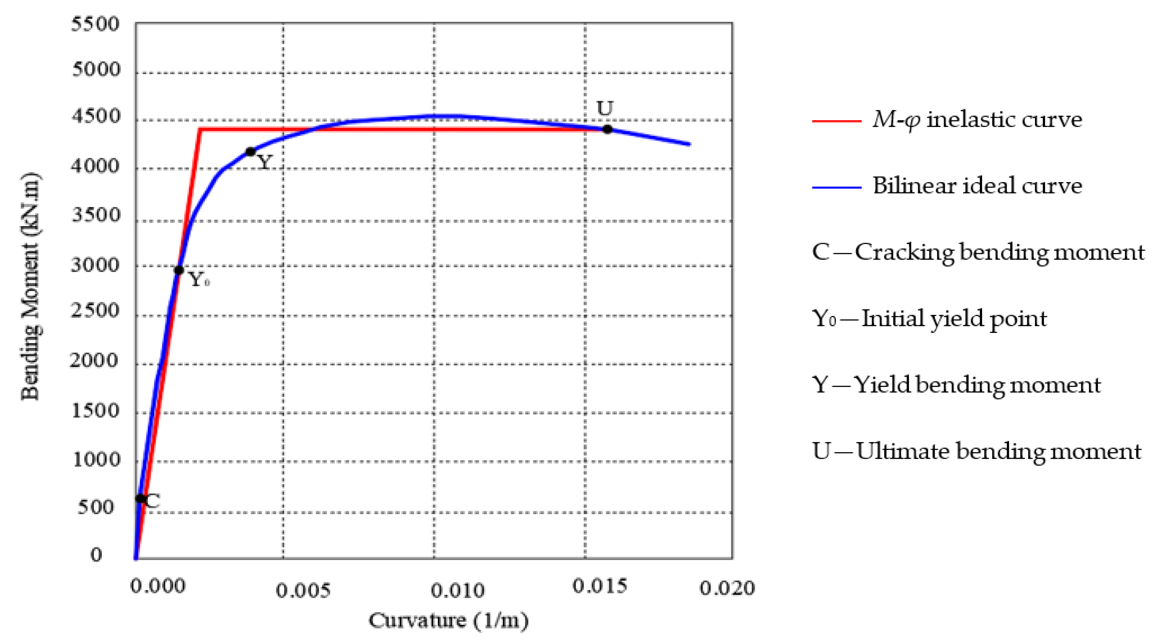
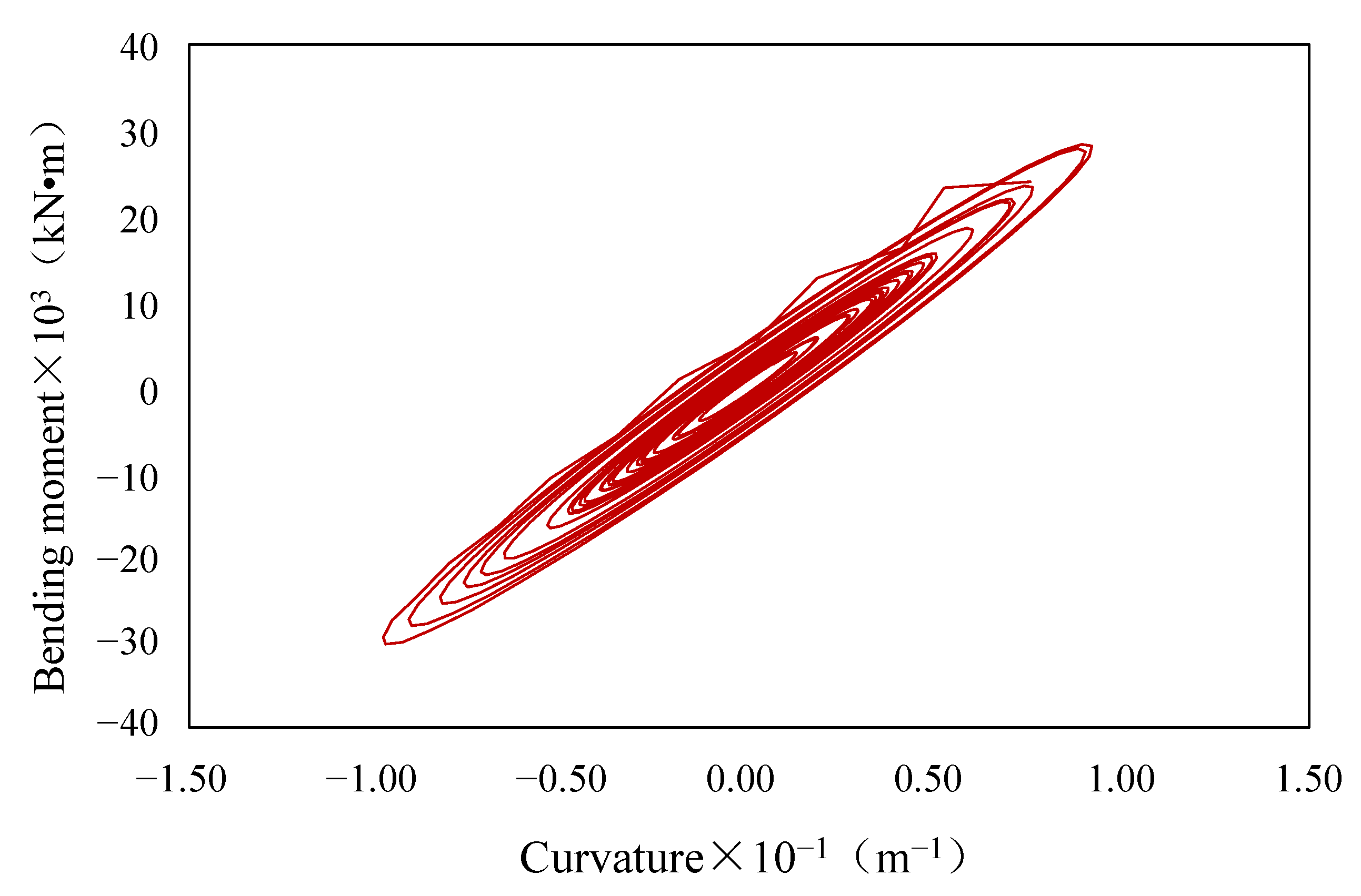
- The proposed approach represents an explicit nonlinear dynamic analysis method. The bending moment–curvature diagram shows an oval shape, which indicates that the central plastic hinge area of the continuous girder bridge pier has significant nonlinear characteristics and can dissipate certain ground motion energy. Under the current Chinese seismic design code, these problems are typical local nonlinear problems (nonlinearities occur near the pier bottom or pier top section with fixed hinges), and the explicit iterative dimension reduction method can be used to ensure the high efficiency of seismic performance evaluation. Compared to the conventional methods, which implicitly solve the equations of motion based on iterative computation involving matrix inversion, the proposed explicit method is expected to have better convergence performance. It is worth noting that the dimension reduction utilizes the unique feature of localized plastic hinges. The dimension reduction method is likely applicable to other nonlinear stochastic dynamic problems involving local plasticity.
- (4)
- The proposed approach has good generality and can be applied to solving similar problems. The kinematic equation of bridge structure is established based on the general dynamic principle. Then, the nonlinear restoring force of the pier column bottom section is described by the Bouc–Wen model, and the nonlinear motion equation of the continuous girder bridge under multi-point seismic excitation is rewritten into a quasilinear equation, which is also established by combining with the Runge–Kutta method and a precise time-history integration method. The explicit dimension reduction iterative method in time domain adopted in this article is essentially a rapid method for solving local nonlinear random vibration of a class of problems, which is applicable as long as the problem can be described as a local nonlinear problem and contains an explicit nonlinear restoring force model. The above methods are not only appropriate to continuous girder bridges, but also applicable to the analysis of similar problems of other bridges.
Author Contributions
Funding
Institutional Review Board Statement
Informed Consent Statement
Data Availability Statement
Conflicts of Interest
References
- Mashal, M.; Palermo, A. Emulative seismic resistant technology for accelerated bridge construction. Soil Dyn. Earthq. Eng. 2019, 124, 197–211. [Google Scholar] [CrossRef]
- Li, X.; Wang, J.; Bao, Y.; Chen, G. Cyclic behavior of damaged reinforced concrete columns repaired with high-performance fiber-reinforced cementitious composite. Eng. Struct. 2017, 136, 26–35. [Google Scholar] [CrossRef]
- Pokhrel, M.; Bandelt, M.J. Plastic hinge behavior and rotation capacity in reinforced ductile concrete flexural members. Eng. Struct. 2019, 200, 109699. [Google Scholar] [CrossRef]
- Jia, J.; Zhao, L.; Wu, S.; Wang, X.; Bai, Y.; Wei, Y. Experimental investigation on the seismic performance of low-level corroded and retrofitted reinforced concrete bridge columns with CFRP fabric. Eng. Struct. 2020, 209, 110225. [Google Scholar] [CrossRef]
- Goel, R.K.; Chopra, A.K. Role of shear keys in seismic behavior of bridges crossing fault-rupture zones. J. Bridge Eng. 2008, 13, 398–408. [Google Scholar] [CrossRef]
- Allam, S.M.; Datta, T.K. Analysis of cable-stayed bridges under multi-component random ground motion by response spectrum method. Eng. Struct. 2000, 22, 1367–1377. [Google Scholar] [CrossRef]
- Atmaca, B.; Yurdakul, M.; Ateş, Ş. Nonlinear dynamic analysis of base isolated cable-stayed bridge under earthquake excitations. Soil Dyn. Earthq. Eng. 2014, 66, 314–318. [Google Scholar] [CrossRef]
- Zhou, Y.; Chen, S. Framework of nonlinear dynamic simulation of long-span cable-stayed bridge and traffic system subjected to cable-loss incidents. J. Struct. Eng. 2016, 142, 04015160. [Google Scholar] [CrossRef]
- Borjigin, S.; Kim, C.W.; Chang, K.C.; Sugiura, K. Nonlinear dynamic response analysis of vehicle–bridge interactive system under strong earthquakes. Eng. Struct. 2018, 176, 500–521. [Google Scholar] [CrossRef]
- Nayfeh, A.H. Perturbation Methods; John Wiley & Sons: Hoboken, NJ, USA, 2008. [Google Scholar]
- Sobiechowski, C.; Socha, L. Statistical linearization of the Duffing oscillator under non-Gaussian external excitation. J. Sound Vib. 2000, 231, 19–35. [Google Scholar] [CrossRef]
- Roberts, J.B.; Spanos, P.D. Random Vibration and Statistical Linearization; Courier Dover Publications: New York, NY, USA, 2003. [Google Scholar]
- Broccardo, M.; Der Kiureghian, A. Nonlinear stochastic dynamic analysis by evolutionary tail-equivalent linearization method. Struct. Saf. 2021, 90, 102044. [Google Scholar] [CrossRef]
- Wang, Z.; Der Kiureghian, A. Tail-equivalent linearization of inelastic multisupport structures subjected to spatially varying stochastic ground motion. J. Eng. Mech. 2016, 142, 04016053. [Google Scholar] [CrossRef]
- Shinozuka, M.; Jan, C.M. Digital simulation of random processes and its applications. J. Sound Vib. 1972, 25, 111–128. [Google Scholar] [CrossRef]
- Su, C.; Huang, H.; Ma, H.; Xu, R. Efficient MCS for random vibration of hysteretic systems by an explicit iteration approach. Earthq. Struct. 2014, 7, 119–139. [Google Scholar] [CrossRef]
- Wang, W.; Zhang, Y.; Ouyang, H. Influence of random multi-point seismic excitations on the safety performance of a train running on a long-span bridge. Int. J. Struct. Stab. Dyn. 2020, 20, 2050054. [Google Scholar] [CrossRef]
- Wen, Y.K. Method for random vibration of hysteretic systems. J. Eng. Mech. Div. 1976, 102, 249–263. [Google Scholar] [CrossRef]
- Truong, D.Q.; Ahn, K.K. MR fluid damper and its application to force sensorless damping control system. In Smart Actuation and Sensing Systems-Recent Advances and Future Challenges; In Tech: Rijeka, Croatia, 2012; pp. 383–425. [Google Scholar]
- Zhong, W.X.; Williams, F.W. A precise time step integration method. Proc. Inst. Mech. Eng. Part C J. Mech. Eng. Sci. 1994, 208, 427–430. [Google Scholar] [CrossRef]
- Xing, Y.; Zhang, H.; Wang, Z. Highly precise time integration method for linear structural dynamic analysis. Int. J. Numer. Methods Eng. 2018, 116, 505–529. [Google Scholar] [CrossRef]
- Yu, F.; Wen, L.; Zhou, F.; Ye, L. Dynamic performance analysis of a seismically isolated bridge under braking force. Earthq. Eng. Eng. Vib. 2012, 11, 35–42. [Google Scholar] [CrossRef]
- Ma, X.; Yang, D.; Song, G. A low-dispersive symplectic partitioned Runge–Kutta method for solving seismic-wave equations: II. Wavefield simulations. Bull. Seismol. Soc. Am. 2015, 105, 657–675. [Google Scholar] [CrossRef]
- Rubinstein, R.Y.; Kroese, D.P. Simulation and the Monte Carlo Method; John Wiley & Sons: Hoboken, NJ, USA, 2016; Volume 10. [Google Scholar]
- Parsons, T. Monte Carlo method for determining earthquake recurrence parameters from short paleoseismic catalogs: Example calculations for California. J. Geophys. Res. Solid Earth 2008, 113. [Google Scholar] [CrossRef]
- JTG 3362-2018; Specifications for Design of Highway Reinforced Concrete and Prestressed Concrete Bridge and Culverts. People’s Communications Publishing House: Beijing, China, 2018. (In Chinese)
- JTG/T 2231-01-2020; Specifications for Seismic Design of Highway Bridges. People’s Communications Publishing House: Beijing, China, 2020. (In Chinese)
- Abbasi, M.; Moustafa, M.A. Effect of damping modeling and characteristics on seismic vulnerability assessment of multi-frame bridges. J. Earthq. Eng. 2021, 25, 1616–1643. [Google Scholar] [CrossRef]
- Salehi, M.; Sideris, P. Enhanced Rayleigh damping model for dynamic analysis of inelastic structures. J. Struct. Eng. 2020, 146, 04020216. [Google Scholar] [CrossRef]
- Clough, R.W.; Penzien, J. Dynamics of Structures, 3rd ed.; McGraw-Hill: New York, NY, USA, 2003. [Google Scholar]
- Jangid, R.S. Stochastic response of bridges seismically isolated by friction pendulum system. J. Bridge Eng. 2008, 13, 319–330. [Google Scholar] [CrossRef]
- Liu, G.; Lian, J.; Liang, C.; Zhao, M. An effective approach for simulating multi-support earthquake underground motions. Bull. Earthq. Eng. 2017, 15, 4635–4659. [Google Scholar] [CrossRef]
- Yang, Q.S.; Tian, Y.J. Earthquake Ground Motions and Artificial Generation; Science Press: Beijing, China, 2008. [Google Scholar]
- Liao, S.; Zerva, A. Physically compliant, conditionally simulated spatially variable seismic ground motions for performance-based design. Earthq. Eng. Struct. Dyn. 2006, 35, 891–919. [Google Scholar] [CrossRef]
- Luco, J.E.; Wong, H.L. Response of a rigid foundation to a spatially random ground motion. Earthq. Eng. Struct. Dyn. 1986, 14, 891–908. [Google Scholar] [CrossRef]


| Area (m2) | Moment of Inertia Iy (m4) | Moment of Inertia Iz (m4) | Elastic Modulus (GPa) | Density (kg/m3) | |
|---|---|---|---|---|---|
| Girder | 12.49 | 6.70 | 228.91 | 34.5 | 2549 |
| Pier | 2.01 | 0.32 | 0.32 | 32.5 | 2549 |
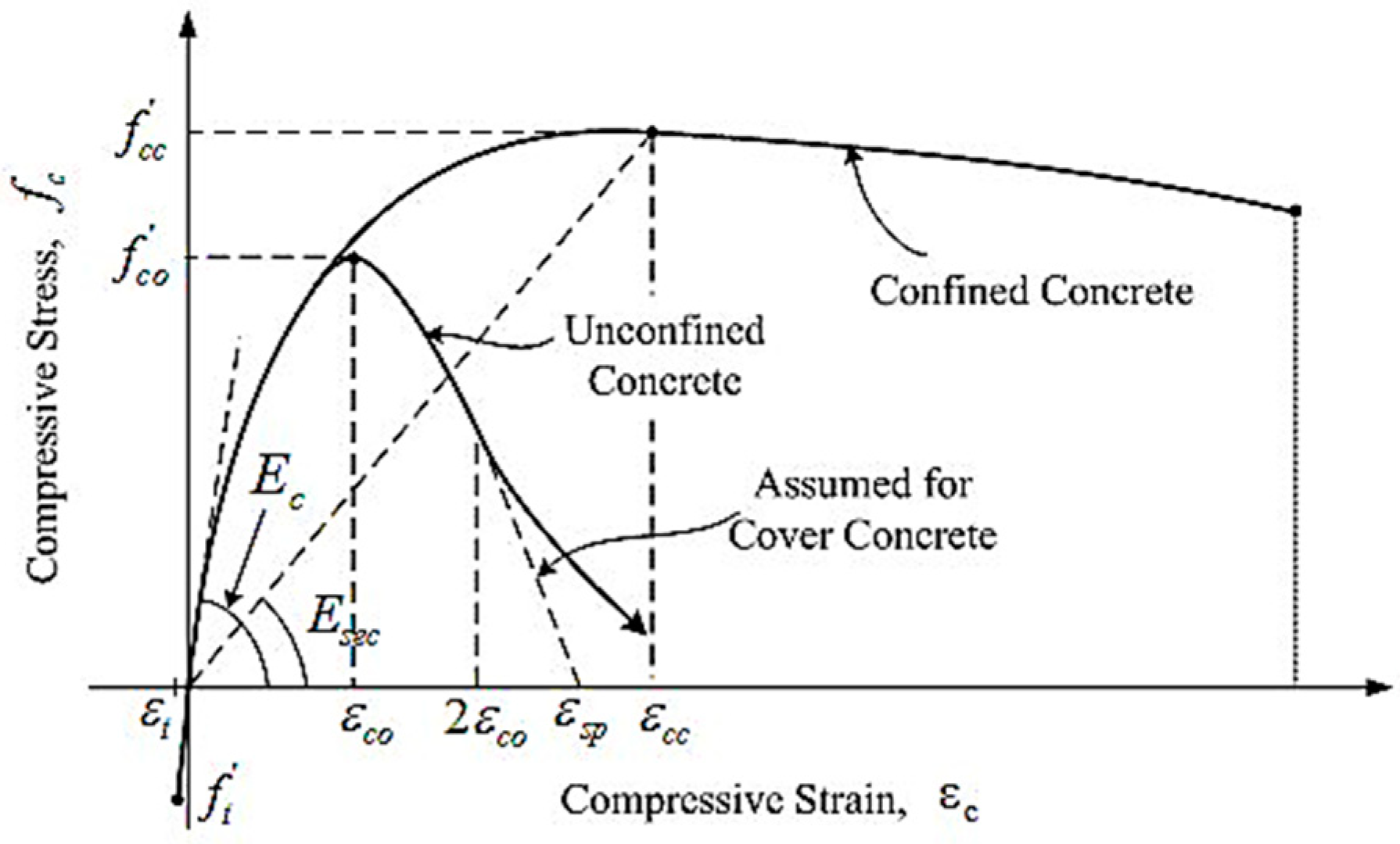
| Type (C40) | Elastic Modulus Ec (MPa) | fc (MPa) | Yield Strain | Peak Strain | Ultimate Strain |
|---|---|---|---|---|---|
| non-confined concrete | 31623 | 40.00 | 0.0014 | —— | 0.02 |
| confined concrete | 31623 | 41.72 | 0.002429 | 0.002 | 0.013084 |
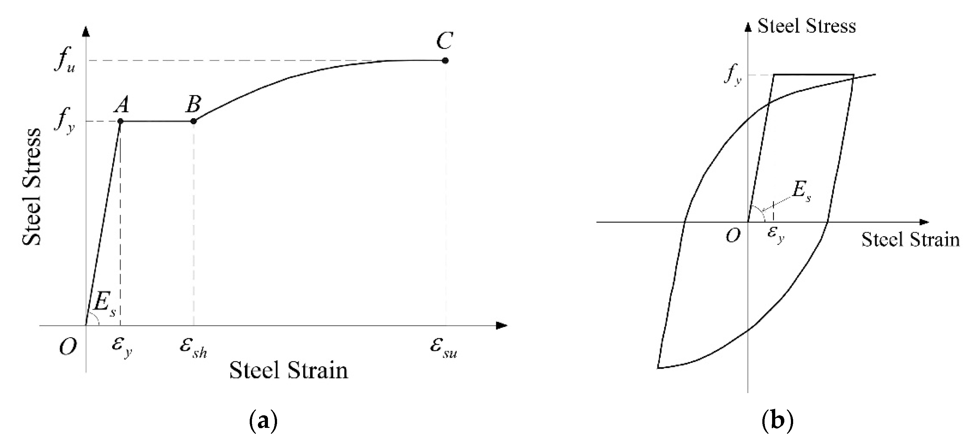
| Type | Es (MPa) | fy (MPa) | fu (MPa) | εy | εsh | εsu |
|---|---|---|---|---|---|---|
| HRB400 | 200,000 | 400 | 540 | 0.002 | 0.01 | 0.1 |
| Site Condition | (rad/s) | (rad/s) | ||
|---|---|---|---|---|
| Soil 1 | 20.94 | 0.6 | 1.5 | 0.6 |
| Soil 2 | 10.0 | 0.4 | 1.0 | 0.6 |
| Method | Time (s) |
|---|---|
| explicit time-domain method | 250 |
| Newmark-β method | 5000 |
| Average Value × 103 (kN·m) | Average Value of the Standard Deviation × 103 (kN·m) | Average Value of the Absolute Maximum × 103 (kN·m) |
|---|---|---|
| 1.89 | 6.22 | 18.04 |
Publisher’s Note: MDPI stays neutral with regard to jurisdictional claims in published maps and institutional affiliations. |
© 2022 by the authors. Licensee MDPI, Basel, Switzerland. This article is an open access article distributed under the terms and conditions of the Creative Commons Attribution (CC BY) license (https://creativecommons.org/licenses/by/4.0/).
Share and Cite
Wei, Z.; Lv, M.; Shen, M.; Wang, H.; You, Q.; Hu, K.; Jia, S. Rapid Seismic Evaluation of Continuous Girder Bridges with Localized Plastic Hinges. Sensors 2022, 22, 6311. https://doi.org/10.3390/s22166311
Wei Z, Lv M, Shen M, Wang H, You Q, Hu K, Jia S. Rapid Seismic Evaluation of Continuous Girder Bridges with Localized Plastic Hinges. Sensors. 2022; 22(16):6311. https://doi.org/10.3390/s22166311
Chicago/Turabian StyleWei, Zhaolan, Mengting Lv, Minghui Shen, Haijun Wang, Qixuan You, Kai Hu, and Shaomin Jia. 2022. "Rapid Seismic Evaluation of Continuous Girder Bridges with Localized Plastic Hinges" Sensors 22, no. 16: 6311. https://doi.org/10.3390/s22166311