Article

Sparse Sliding-Window Kernel Recursive Least-Squares Channel Prediction for Fast Time-Varying MIMO Systems

1
ZTE Corporation, Algorithm Department, Wireless Product R&D Institute, Wireless Product Operation Division, Shenzhen 518057, China
2
Key Laboratory of Universal Wireless Communications, Ministry of Education of China, Beijing University of Posts and Telecommunications, Beijing 100876, China
*
Author to whom correspondence should be addressed.
Sensors 2022, 22(16), 6248; https://doi.org/10.3390/s22166248
Submission received: 10 June 2022 / Revised: 29 July 2022 / Accepted: 13 August 2022 / Published: 19 August 2022
(This article belongs to the Special Issue Resource Allocation for Cooperative Communications)

Abstract

:
Accurate channel state information (CSI) is important for MIMO systems, especially in a high-speed scenario, fast time-varying CSI tends to be out of date, and a change in CSI shows complex nonlinearities. The kernel recursive least-squares (KRLS) algorithm, which offers an attractive framework to deal with nonlinear problems, can be used in predicting nonlinear time-varying CSI. However, the network structure of the traditional KRLS algorithm grows as the training sample size increases, resulting in insufficient storage space and increasing computation when dealing with incoming data, which limits the online prediction of the KRLS algorithm. This paper proposed a new sparse sliding-window KRLS (SSW-KRLS) algorithm where a candidate discard set is selected through correlation analysis between the mapping vectors in the kernel Hilbert spaces of the new input sample and the existing samples in the kernel dictionary; then, the discarded sample is determined in combination with its corresponding output to achieve dynamic sample updates. Specifically, the proposed SSW-KRLS algorithm maintains the size of the kernel dictionary within the sample budget requires a fixed amount of memory and computation per time step, incorporates regularization, and achieves online prediction. Moreover, in order to sufficiently track the strongly changeable dynamic characteristics, a forgetting factor is considered in the proposed algorithm. Numerical simulations demonstrate that, under a realistic channel model of 3GPP in a rich scattering environment, our proposed algorithm achieved superior performance in terms of both predictive accuracy and kernel dictionary size than that of the ALD-KRLS algorithm. Our proposed SSW-KRLS algorithm with M = 90 achieved 2 dB NMSE less than that of the ALD-KRLS algorithm with v = 0.001 , while the kernel dictionary was about 17% smaller when the speed of the mobile user was 120 km/h.

1. Introduction

Multiantenna technology can fully use spatial dimension resources and dramatically improve the capacity of wireless communication systems without increasing transmission power and bandwidth [1]. Meanwhile, beamforming technology [2,3] is widely used to reduce the interference between cochannel users with cooperative transmission and reception since it can compensate channel fading and distortion caused by the multipath effect. Base stations optimize the allocation of radio resources through reasonable precoding, rendering the desired signal and interference more orthogonal provided that CSI is known at the base station. Thus, the acquisition of CSI is very important in the cooperation of transmission and reception [4]. However, due to the dynamics of the channel, especially when the terminal is moving at a high speed, the acquisition of CSI is a formidable problem in MIMO systems.
In TDD systems, the user sends a sounding reference signal (SRS), and the base station performs channel estimation algorithms such as LS [5] and MMSE [6]. Then, the obtained CSI is used for downlink beamforming to realize cooperative signal processing. The coherence time of wireless channels is the time duration after which CSI is considered to be outdated. When the terminal is moving at a high speed, the Doppler frequency shift grows, and the time variability of the channel is severe, which leads to the shortening of channel coherence time. The measured uplink channel CSI cannot represent the real channel state of downlink slots, resulting in the mismatch between the downlink beamforming designed according to the measured CSI and the actual channel. In [1], with a typical CSI delay of 4 milliseconds, the user terminal speed at 30 km/h led to as much as 50% performance reduction versus in the low-mobility scenario at 3 km/h.
In order to overcome the performance degradation caused by severe time-varying channels, [7] proposed a tractable user-centric CSI model and a robust beamforming design by taking deterministic equivalents [8] into account. However, when the user terminal is at high speed, the channel shows nonstationary characteristics, and the statistical characteristics of the channel also change with time, which cannot be used for the beamforming of high-speed time-varying channels.
Another approach is to use a channel prediction algorithm [9,10,11,12,13,14,15,16] to obtain more accurate CSI for beamforming. The kernel method is widely used in channel prediction algorithms due to its ability to track nonlinear channels, and its adaptation to time-varying channels [17,18,19,20,21,22]. However, algorithms based on kernel methods face the problem in online prediction that the networks structure grows as the size of the training samples grows in time. Though researchers have proposed sparseness methods to limit the size of samples by setting prerequisites for new samples added into the dictionary, the size of the kernel dictionary cannot be precisely controlled. Therefore, this paper proposes a new channel algorithm based on the kernel method that maintains the size of the kernel dictionary within a fixed budget while precisely tracking the fast time-varying dynamic characteristics.

1.1. Related Work

State-of-the-art channel fading prediction algorithms were reviewed in [9]. Parametric radio channel-based methods [10] consider channel changes faster than multipath parameters, and the estimation of these parameters can help in the extrapolation of the channel into future. However, the effective time of static multipath parameters is inversely proportional to the terminal moving speed, rendering the channel prediction based on radio parameters not appropriate for high-speed scenarios. Autoregressive (AR) model-based methods [11,13] do not explicitly model physical scatterings, considering the time-varying channel as a stochastic wide-sense stationary (WSS) process and the temporal autocorrelation function is used for prediction. Nevertheless, they are not capable of predicting ephemeral variations in non-wide-sense-stationary (NWSS) channels due to their linear correlation assumption. When treating NWSS channels, many studies attempted to use machine learning in channel prediction. The authors in [14] proposed a backpropagation (BP) framework regarding channel prediction for backscatter communication networks that considers both spatial and frequency diversity. In [15], the authors developed a machine-learning method for predicting a mobile communication channel on the basis of a specific type of convolutional neural network. Although these algorithms can achieve good performance, they need to build neural networks, require a large number of samples for training, and the complexities of these algorithms are high. The channel prediction method based on a support vector machine [16,23] uses Mercer’s theorem [24] to map the channel sample space to the high-dimensional space, and performs linear regression in the high-dimensional space to solve the problem of tracking nonlinear channels well. The kernel recursive least-squares (KRLS) [17,18,19,20,21,22] algorithm is a nonlinear version of the recursive least-squares (RLS) algorithm. It can not only solve nonlinear problems, but also adaptively iterate the model parameters.
In order to solve this problem and render the online kernel method feasible, researchers proposed various sparseness methods or criteria, such as approximate linear dependency (ALD) [17], the novelty criterion (NC) [20], the surprise criterion (SC) [21], and the coherence criterion (CC) [22]. On the basis of these sparseness methods or criteria, only new input samples that meet the prerequisites are added to the dictionary. However, these sparse methods cannot precisely control the size of the kernel dictionary, which motivated us to introduce a sliding window to control the size of the kernel dictionary. Recently, some KRLS-based algorithms with an inserted forgetting factor have achieved better performance than that of QKRLS algorithms [25,26] and ALD-KRLS, which motivated us to insert a forgetting factor into the proposed SSW-KRLS algorithm. This paper proposes a new sparse sliding-window KRLS algorithm where a candidate discard set is selected through correlation analysis between the mapping vectors in the kernel Hilbert spaces of the new input sample and the existing samples in the kernel dictionary; then, the discarded sample is determined in combination with its corresponding output to achieve dynamic sample updates.

1.2. Contributions

The main contributions of this paper are summarized as follows:
  • We propose a novel sparse sliding-window KRLS algorithm. To precisely control the size of samples, we introduce a sample budget as a size restriction. When the dictionary was smaller than the sample budget, we directly added the new sample to the dictionary. Otherwise, we chose the best sample to discard according to our proposed new criterion.
  • To differentiate the sample value collected at different times, we introduced a forgetting matrix. By setting different forgetting values for samples collected at different times, we quantified the time value of the samples. The older sample had a smaller forgetting value, which means that its time value was smaller. In this way, we considered both the correlation of samples and the time value when discarding old samples.
  • Regarding our new method for discarding old samples, we set a candidate set where we decided which sample to discard. The candidate set was obtained by adding the samples that had larger kernel functions of the new sample than a threshold and were highly correlated with the new sample. Then, we conducted a weighted estimation of the output value of these samples. We decided which sample to discard on the basis of the deviation between its output and the estimated value.
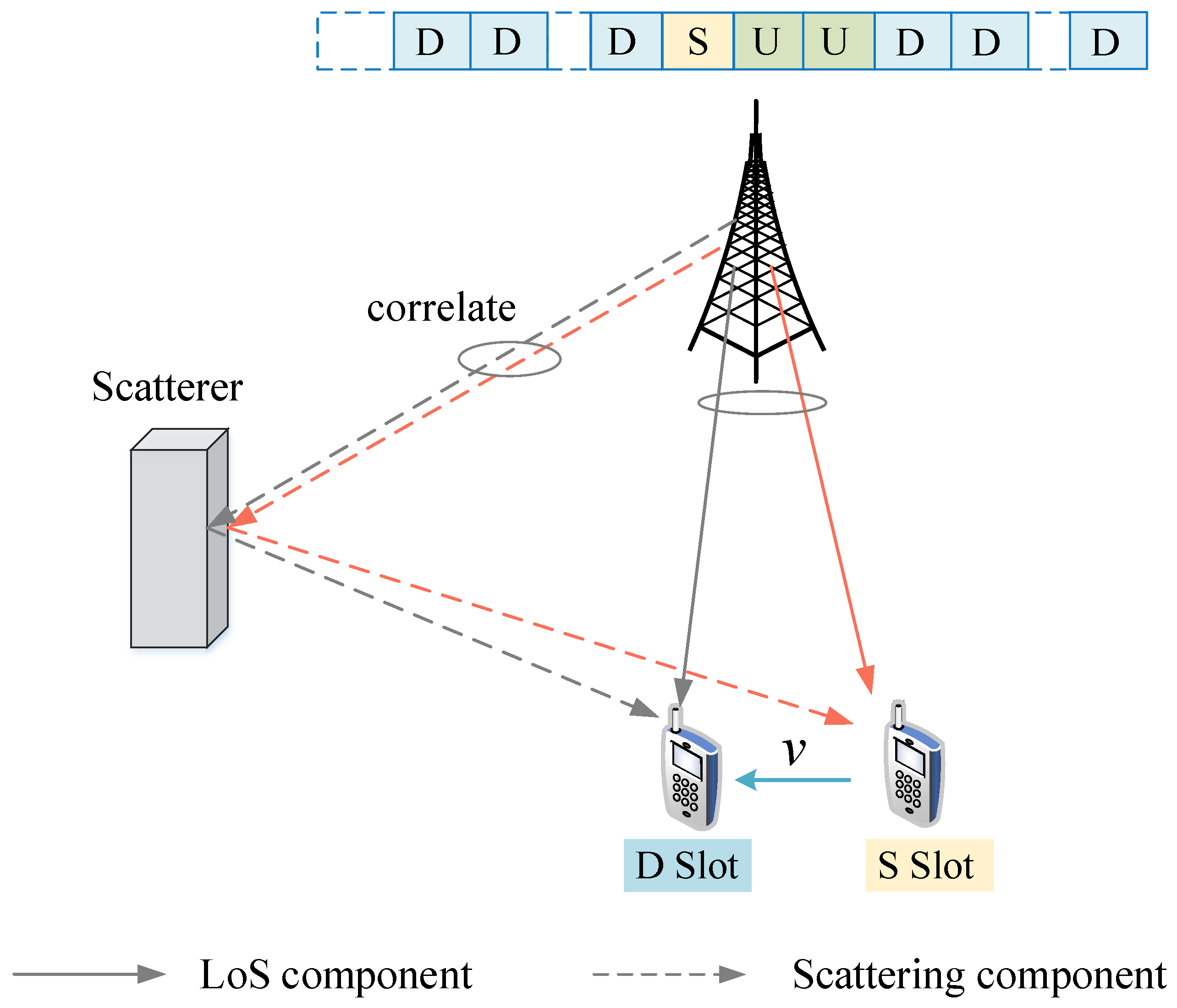
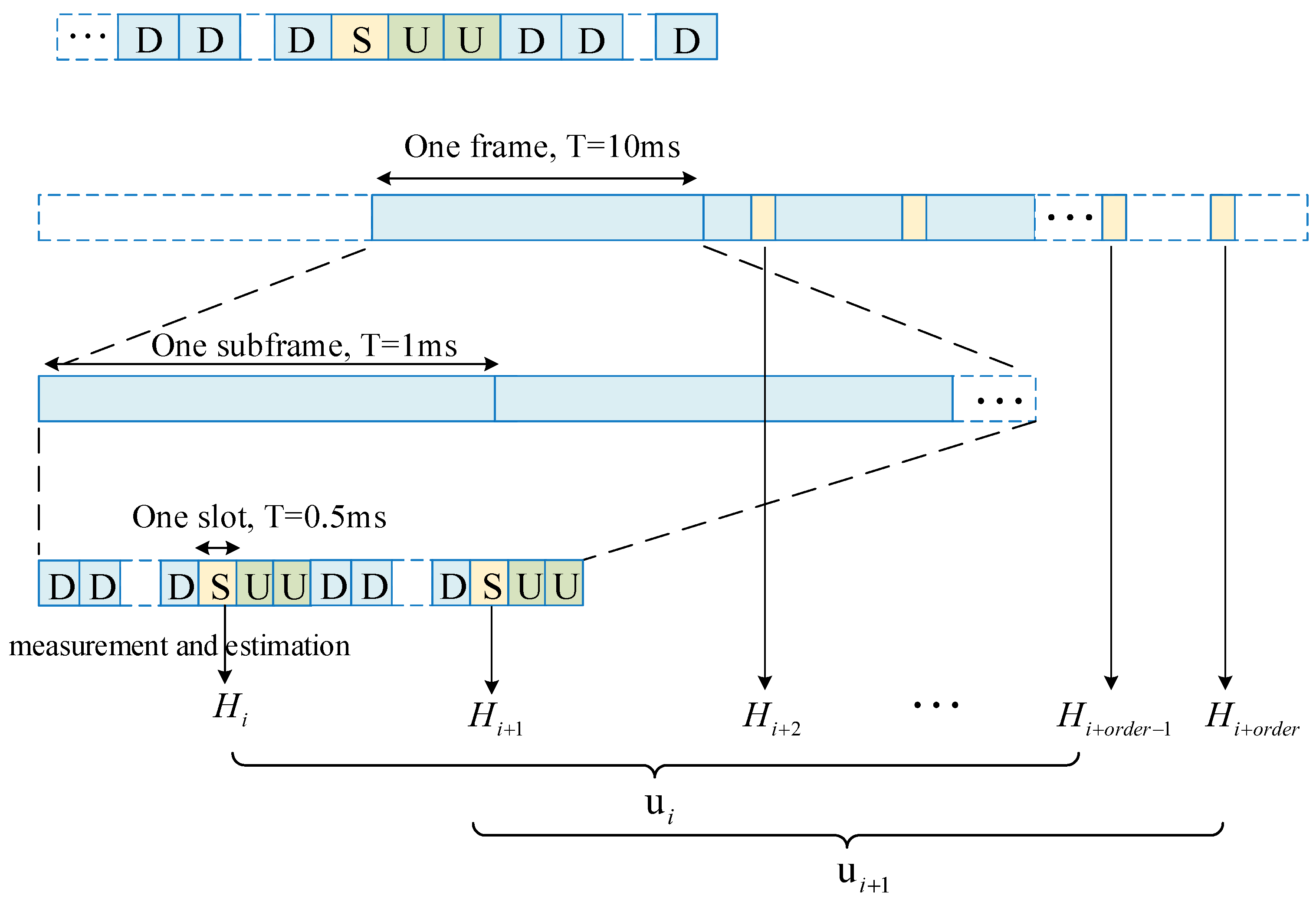
2. System Model

We considered two typical user movement scenarios: urban road where the moving speed of users is 60 km/h, and a highway where the moving speed of users is 120 km/h. As shown in Figure 1, in TDD systems, the user sends a SRS, and the base station runs channel estimation algorithms such as LS and MMSE. The channel matrix is first estimated in frequency-domain; then, the channel frequency response is transformed into the time-domain by IDFT. The noise is evenly distributed in the whole time domain and is easy to be eliminated using a raised cosine window. Therefore, the effect of noise is very small compared to the user’s high mobility. Due to the channel reciprocity in TDD systems, uplink channel CSI can be directly used in the design of downlink beamforming to realize cooperative signal processing. However, nonstationary fast fading characteristics of mobile environments bring challenges to multi-input multi-output (MIMO) communications.
When the terminal is moving at a high speed, the Doppler frequency shift grows, and the time variability of the channel is severe. The measured uplink channel CSI cannot represent the real channel state of the downlink slots, resulting in performance degradation, and a mismatch between the measured CSI and the actual channel. As shown in Figure 2, during the SRS reporting cycle, the user can be regarded as moving in a fixed direction at a fixed speed. In two adjacent time slots, due to the short moving distance of the user, the amplitude and phase of the direct and scattered components have a certain correlation. When the user speed is low, an AR-based channel prediction method can achieve good performance by utilizing the linear correlation between adjacent time slots. However, when the user is moving at a high speed, the channel correlation between adjacent time slots presents nonlinear characteristics. Kernel methods are needed to exploit the nonlinear correlation characteristics of the channel.
The user sends SRS in special time slots, and the BS performs the channel measurement and estimation to obtain the channel matrix. As shown in Figure 3, the channel matrix measured by BS in the i-th SRS period is assumed to be H i C N r × N t . N t and N r represent the number of antennas of the BS and the mobile UE, respectively. The real and imaginary parts are separately processed in the subsequent algorithm, and H represents a real matrix in the later representation. The prediction order means that each channel matrix is related to the channel matrix measured in the previous-order SRS periods, so the input vector of the prediction system is
u i = H i , H i + 1 , , H i + o r d e r 1 .
There are some complex and unknown dependencies between u i and H i : H i + o r d e r 1 = f u i = f H i , H i + 1 , , H i + o r d e r 1 that need to be exploited by kernel methods.

3. Traditional KRLS Algorithm

In this section, we introduce the traditional KRLS algorithm and several extensions to the KRLS algorithm.

3.1. Traditional KRLS Algorithm

Assume a set of ordered input-output pairs D = u i , y i | i = 1 m , where m is the total number of samples, u i R m are m-dimensional input vectors and y i R is the output. We call D a dictionary that records the input-output pairs collected before the i-th time slot. First, according to the Mercer theorem, we can adopt a nonlinear function φ ( · ) to transform data u i R m into a high-dimensional feature space: φ ( · ) : R m R c . The corresponding kernel function is κ u , v = φ u , φ v . We need to minimize the cost function:
J = j = 1 i y i w i φ j 2 = Φ i T w i y i 2 ,
where Φ i = φ u 1 , . . . , φ u i = φ 1 , , φ i is a high-dimensional matrix. By minimizing the cost function as (2), we can obtain weight w i = Φ i y i , where Φ i is the pseudoinverse of Φ i . Φ i cannot be solved directly because kernel function κ u , v is a high-dimensional mapping, and the exact mapping function is unknown. To avoid overfitting when the samples are small, we used L2 regularization, so the cost function is reformulated as:
J = Φ i T w i y i 2 + λ w i 2 .
By letting J w i = 0 , we can obtain that
w i = Φ i [ λ I + Φ i T Φ i ] 1 y i = Φ i α ( i ) .
By substituting (4) into (3), the cost function can be reformulated as:
J = Φ i T Φ i α ( i ) y i 2 + λ w i 2 = K i α ( i ) y i 2 + λ w i 2 ,
where K i is the kernel matrix and the element located at the i-th row and j-th column of K i is K i i , j = κ u i , u j . The problem is to solve
α ( i ) = [ λ I + Φ i T Φ i ] 1 y i = [ λ I + K i ] 1 y i = Q ( i ) y i ,
Then, the inverse of Q ( i ) can be obtained as:
Q ( i ) 1 = λ I + K i = Q ( i 1 ) 1 k i k i T λ + κ u i , u i ,
where k i = Φ i 1 T φ i . Thus, Q ( i ) can be solved using the inversion of the partitioned matrix.
Q ( i ) = r ( i ) 1 Q ( i 1 ) r ( i ) + z ( i ) z ( i ) T z ( i ) z ( i ) T 1 ,
where z ( i ) = Q ( i 1 ) k i and r ( i ) = λ + φ i T φ i z ( i ) 1 φ i .
The traditional KRLS algorithm is summarized in Algorithm 1.
Algorithm 1 Traditional KRLS algorithm.
1:
Initialize Q ( 1 ) = λ + k ( u 1 , u 1 ) 1 and α ( 1 ) = Q ( 1 ) y 1 .
2:
Iterate for i > 1: k i = Φ i 1 T φ i , z ( i ) = Q ( i 1 ) k i , r ( i ) = λ + φ i T φ i z ( i ) 1 φ i ,
Q ( i ) = r ( i ) 1 Q ( i 1 ) r ( i ) + z ( i ) z ( i ) T z ( i ) z ( i ) T 1
By relying on the kernel trick, the traditional KRLS algorithm can deal with nonlinear problems by nonlinearly transforming data into a high-dimensional reproducing kernel Hilbert space, which is similar to other techniques such as support vector machines (SVMs). Compared to SVMs, it avoids large-scale high-dimensional computing through iterative computations. However, the traditional KRLS algorithm grows linearly with the number of processed data, rendering growing complexities for each consecutive update if no additional measures are taken. In order to render online kernel algorithms feasible, growth is typically slowed down by approximately representing the solution using only a subset of bases that are considered to be relevant according to a chosen criterion. In our proposed SSW-KRLS algorithm, we took similar operations to avoid an increase in computation, which is discussed in detail in Section 4.

3.2. Extensions to KRLS Algorithm

The kernel recursive least-squares method is one of the most efficient online kernel methods, and it achieves good performance in nonlinear fitting and prediction. However, the bottleneck problem is that the network structure grows with the training samples, which leads to insufficient memory and computational complexities when processing continuously incoming signals. In order to solve this problem and render the online kernel method feasible, researchers have proposed various sparseness methods or criteria, such as approximate linear dependency (ALD), the novelty criterion (NC), the surprise criterion (SC) and the coherence criterion (CC). On the basis of these sparseness methods or criteria, only new input samples that meet the prerequisites are used as training samples. Thus, the growth of network structure is effectively slowed down. Table 1 shows several common sparseness criteria.
The performance of the above methods in filtering samples largely depends on the selected threshold. As time goes by, the number of samples increases slowly and lastly stabilizes, while the update of model parameters tends to be slow. This is not conducive to updating time-varying channels. Furthermore, when the user moves into a new environment, the outdated samples are reserved, which is not conducive to channel prediction.
An effective way to keep the dictionary updated while precisely controlling its size is using the sliding window. A simple implementation is discarding the oldest sample directly each time a new sample is collected, but it lacks the judgement of correlation between samples. Sparseness simply based on time information is unreliable and may result in unstable prediction performance when the window is small. In order to solve this problem, we propose a new algorithm, SSW-KRLS, where we take both the time value and correlation between samples into consideration.

4. Proposed SSW-KRLS Algorithm

Assume that there is a set of input–output pairs D = u i , y i | i = 1 L where L is the total number of samples. u i R m are m-dimensional input vectors, and y i R is the output. In the traditional KRLS algorithm, in each time slot, when a new sample comes, the size dictionary increases, and this leads to an increase in computation and memory requirements. To solve this problem, we used a sliding-window approach to keep the size of the kernel dictionary within a fixed budget. Our criterion for discarding old samples was based on the correlation between existing samples in the kernel dictionary and the new sample. Moreover, we introduced a forgetting factor to exponentially weigh older data by scaling them, so as to track the dynamic characteristics of the channel.
In our proposed SSW-KRLS algorithm, we solved the following least-squares cost function:
min w j = 1 i β i j y j w T φ j 2 + λ B ( i ) w T w ,
where β is the forgetting factor, and i is the iteration number, y i = ( y 1 , . . . , y i ) T is the output vector, w is the weight vector, B ( i ) = d i a g ( β L 1 , β L 2 , , 1 ) is the forgetting matrix, φ j = φ u j is the transformation of u j , and λ is the regularization parameter. The optimal w * is solved:
w * = λ B ( i ) + Φ i B ( i ) Φ i T 1 Φ i B ( i ) y i .
We reformulate the equation:
w * = Φ i λ B ( i ) + B ( i ) K i 1 y i ¯ ,
where y i ¯ = B ( i ) y i is the exponentially weighted input signal.
The solutions for Q ( i ) = λ B ( i ) + B ( i ) K i 1 are different under two cases in the i-th iteration: one case is that the size of the dictionary increased, and the other is that the size of the dictionary remained unchanged. Cases I and II are discussed in Section 4.2 and Section 4.3, respectively. In Section 4.1, we introduce how to update our dictionary when a new sample comes. Our methods are different depending on whether the size of the dictionary reaches the fixed sample budget, which is denoted by M. In particular, when the dictionary was not full, we discarded an old sample on the basis of the correlation analysis between the new and existing samples in the dictionary in order to slow down the increase in dictionary size. In the case when the size of the dictionary was full, we set a candidate discard set which contains the samples highly correlated with the new sample, and determine which sample to discard on the basis of their corresponding output. The whole process of our proposed algorithm is shown in Figure 4.

4.1. How to Optimally Discard an Old Sample

The cosine value is usually adopted for judging the correlation of two vectors. In the KRLS algorithm, on the other hand, the cosine value is calculated in the kernel Hilbert spaces. Suppose u i is a new sample, and u j is an existing sample in the dictionary. Let k ( u j ) denote the kernel vector of u j D . k ( u j ) = { k j n } n i , j , where k j n = κ u j , u n . To measure the correlation between the existing and new samples, we calculated the cosine value of k u i and k u j for u j D , as cos k ( u i ) , k ( u j ) = k ( u i ) k ( u j ) T k ( u i ) k ( u j ) . When the size of the dictionary did not reach the budget, we found a sample with highest correlation with the new sample. Existing sample u j that had the highest cosine value was the most probable to be discarded, where j = arg max j cos k ( u i ) , k ( u j ) . We set a threshold τ and discarded sample u j if cos k ( u i ) , k ( u j ) τ . The updated dictionary is:
D ( i ) = D ( i 1 ) \ u j , u i , i f max j cos k ( u i ) , k ( u j ) τ D ( i 1 ) , u i , i f max j cos k ( u i ) , k ( u j ) < τ
In another case, when the size of the dictionary reaches the fixed budget, one sample must be discarded from the kernel dictionary in each time slot. In our strategy, we first set a candidate discard set on the basis of the correlation with the new sample, and then determined the optimal discarded sample according to its output value.
Candidate discard set S was composed of the samples that had high correlation with the new sample. Specifically, an existing sample in dictionary u j D was added into S if κ ( u i , u j ) > ε , where u i is a new sample and ε is a threshold. Among the samples in S, the one with the smallest value for prediction may be one that has the most similar information with the new sample or the one that is untypical with little probability to occur. We determined the discarded sample in combination with its corresponding output as following.
Suppose that the candidate discard set is S = u 1 , u 2 , , u n . The weighted average of the output values can be obtained as y = j = 1 n w j y j where
w j = κ ( u i , u j ) j = 1 n κ ( u i , u j )
and n is the number of samples in S.
The deviation between the output value of u j S and the weighted average output value is e j = y j y . The sample with maximal deviation e max is not typical and may have occurred with a small probability, while the one with minimal deviation had similar information to that of the new sample. Suppose that the sample with the maximal deviation is u j m a x , and the sample with the minimal deviation is u j m i n . We chose one of these two samples to discard according to the production of e max and e min . If the production of e max and e min was larger than threshold τ , this indicated that e max was large enough, so we discarded u j m a x ; otherwise, e min was small enough, and we discarded u j m i n . The updated dictionary is:
D ( i ) = D ( i 1 ) \ u j m a x u i , i f e max e min τ D ( i 1 ) \ u j m i n u i , i f e max e min < τ .

4.2. Case I: The Size of D ( i ) Is Changed

As mentioned before, the prediction process depends on whether the size of the dictionary has increased or not. In Case I, when the size of dictionary increased, we could obtain from (11) that:
w i = Φ i α ( i ) α ( i ) = Q ( i ) y ¯ i Q ( i ) = λ B ( i ) + B ( i ) K i 1 .
With the combination of B ( i ) and y i , we could obtain exponentially weighted input signal y ¯ i . We can find that
B ( i ) = β B ( i 1 ) 0 0 T 1
K i = K i 1 h ( i ) h ( i ) T κ ( u i , u i )
y ¯ i = β y ¯ i 1 y ¯ i ,
where h ( i ) = κ ( u 1 , u i ) , κ ( u 2 , u i ) , , κ ( u i 1 , u i ) T . Thus
B ( i ) K i = β B ( i 1 ) K i 1 β B ( i 1 ) h ( i ) h ( i ) T κ ( u i , u i )
By substituting (19) into (15), we can obtain that
Q ( i ) = β Q ( i 1 ) 1 β B ( i 1 ) h ( i ) h ( i ) T κ ( u i , u i ) + λ 1
With partitioned matrix inversion, we can obtain Q ( i ) in recursive form:
Q ( i ) = r ( i ) 1 β 1 r ( i ) Q ( i 1 ) + β 1 z B ( i ) z ( i ) T z B ( i ) β 1 z ( i ) T 1 ,
where
z B ( i ) = Q ( i 1 ) B ( i 1 ) h ( i ) r ( i ) = κ u i , u i + λ h ( i ) T z B ( i ) z ( i ) = Q ( i 1 ) T h ( i )
α ( i ) = α ( i 1 ) z B ( i ) r ( i ) 1 e ( i ) r ( i ) 1 e ( i ) ,
and e ( i ) = y i h ( i ) T α ( i 1 ) is the prediction error in the i t h time slot.

4.3. Case II: The Size of D ( i ) Is Unchanged

In the case when the size of the dictionary did not change, the information of the discarded sample u j * in Q ( i 1 ) needed to be deleted. The information of u j * lay in the j * t h column and j * t h row of Q ( i 1 ) . In order to not influence the update of the matrix, we moved the j * t h column and j * t h row of Q ( i 1 ) into the first row and the first column, and obtained Q ^ ( i 1 ) . Correspondingly, we applied the same transformation to K i 1 and obtained K ^ ( i 1 ) . For Q ( i 1 ) = λ B ( i 1 ) + B ( i 1 ) K i 1 1 ; after the movement, the j t h column that meets j < j * should be multiplied by β .
Suppose that the matrix after removing the first column and first row of Q ^ ( i 1 ) and K ^ ( i 1 ) is Q ˜ ( i 1 ) and K ˜ ( i 1 ) , respectively. We can obtain its inversion Q ˜ ( i 1 ) 1 according to Appendix B,
Q ^ ( i 1 ) = e f T l G
Q ˜ ( i 1 ) 1 = G l f T / e .
New matrix Q ( i ) can be formulated into a partitioned matrix:
Q ( i ) = β Q ˜ ( i 1 ) 1 β B ( i 1 ) K i k ( i ) T κ ( u i , u i ) + λ 1 = A b p T κ ( u i , u i ) + λ 1 .
Then, Q ( i ) can be obtained using the partitioned matrix:
Q ( i ) = λ β i I ( i ) + B ( i ) K i 1 = A 1 ( I + b p T A 1 g ) A 1 b g p T A 1 g g ,
where A 1 = β 1 K ˜ ( i 1 ) 1 B ( i 1 ) 1 , g = ( κ ( u i , u i ) + λ p T A 1 b ) 1 .
Then, the weight coefficient is updated:
α ( i ) = Q ( i ) y ¯ i = Q ( i ) B ( i ) y i ,
where y i is composed of the output value of the samples y i = y 1 , y 2 , , y i T . Lastly, we can obtain the prediction value for the next time slot as y ^ i + 1 = α ( i ) k ( i ) T .

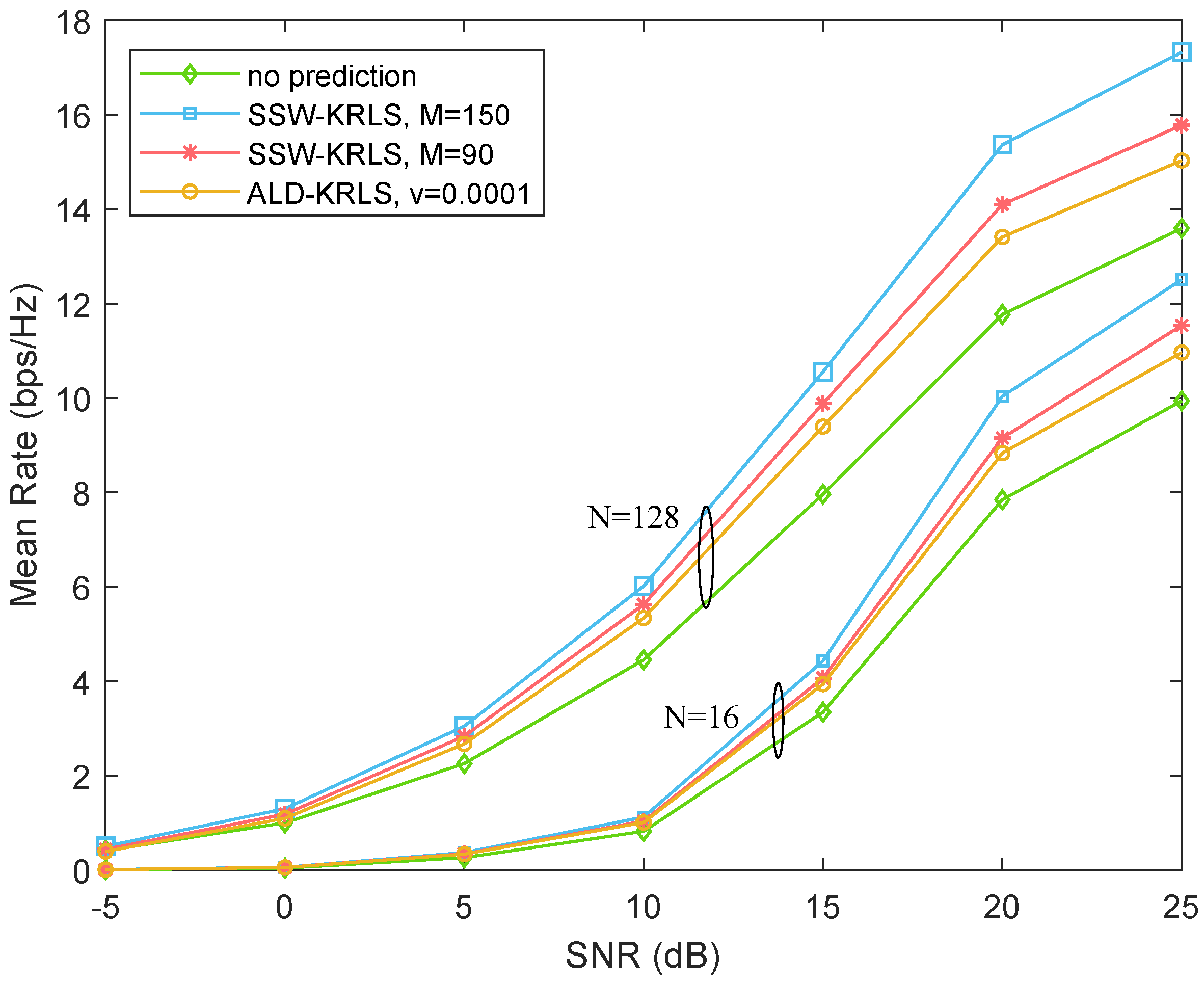
5. Performance Evaluation

Based on the analysis above, we present algorithmic steps as Algorithm Section 5 and in this section we show the simulation results of our proposed SSW-KRLS algorithmcompare its performance to that of the ALD-KRLS algorithm as a baseline. The basic simulation parameters are listed in Table 2. We adopted a 3D urban macro scenario, and considered a typical setting of 3 kHz with 30 kHz of subcarrier spacing. We considered 20 MHz of bandwidth that contained 51 resource partitions. Our adopted channel model was a CDL-A channel model, and the DL precoder was RZF.
Algorithm 2 Proposed SSW-KRLS algorithm.
1:
Initialize Q ( 1 ) = λ + κ ( u 1 , u 1 ) 1 , B ( 1 ) = 1 , α ( 1 ) = Q ( 1 ) y 1 , D ( 1 ) = u 1 .
2:
Step 1: Iterate for i > 1 : judging the number of samples in D ( i ) , which is L. If L < M , perform Step 2; otherwise, perform Step 3.
3:
Step 2: For each sample u j in D ( i 1 ) , compute cos k ( u i ) , k ( u j ) .
Find j * = arg max j cos k ( u i ) , k ( u j ) .
If max j cos k ( u i ) , k ( u j ) > τ , discard u j * . Then, add new sample u i into the dictionary. Turn to Step 4.
4:
Step 3: Construct candidate discard set S. Suppose S = u 1 , u 2 , , u n . Then, calculate the output of the samples.
For each sample u j , calculate e j = y j y . Find j m a x = arg max j e j and j m i n = arg min j e j .
If e min e max > τ , D ( i ) = D ( i 1 ) \ u j m a x , u i .
If e min e max τ , D ( i ) = D ( i 1 ) \ u j m i n , u i .
Turn to Step 4.
5:
Step 4: If D ( i ) is larger than D ( i 1 ) , perform Step 5; otherwise, perform Step 6.
6:
Step 5: Calculate Q ( i ) according to (21) and then calculate intermediate matrix z B ( i ) , r ( i ) , z ( i ) according to (22). Calculate α ( i ) according to (23). The prediction value for the next time slot is y ^ i + 1 = α ( i ) k ( i ) T .
7:
Step 6: For Q ( i 1 ) moving the j * t h column and j * t h row into the first column and the first row, and obtain Q ˜ ( i 1 ) ; calculate Q ˜ ( i 1 ) 1 by (24) and (25).
Update Q ( i ) according to (26) and (27). Then, the prediction value is obtained on the basis of (28).
Figure 5 shows the normalized mean squared error (NMSE) performance of different algorithms. We show the performance of the ALD-KRLS and SSW-KRLS algorithms with the 60 and 120 km/h velocity levels for all UEs. When the UE speed was 60 km/h, the prediction algorithms was more accurate than with a UE speed of 120 km/h. Regarding the performance of the SSW-KRLS algorithm, we set different sample budgets: M = 30 , 90 , 150 . The algorithm performed better with a higher sample budget. The SSW-KRLS algorithm with sample budget M = 30 performed better than the ALD-KRLS algorithm with v = 0.001 , and the SSW-KRLS algorithm with sample budget M = 90 greatly outperformed the ALD-KRLS algorithm. However, the performance was insignificantly improved when changing the sample budget from 90 to 150.
Figure 6 shows the kernel dictionary size with 400 iterations. The kernel dictionary size for all algorithms first grew and then slowed down; the size for SSW-KRLS remained unchanged. The SSW-KRLS algorithm with sample budget M = 90 outperformed the ALD-KRLS algorithm with v = 0.001 , while the former used fewer samples. This indicates the superiority of our proposed SSW-KRLS algorithm.
Figure 7 and Figure 8 show the mean rate of mobile users under different algorithms at the speed of 60 and 120 km/h, respectively. Comparing the figure at two speed levels shows that the user with the lower speed had a higher mean rate. In addition, the performance could be enhanced greatly with the use of the channel prediction algorithm. Particularly, our proposed SSW-KRLS algorithm with sample budgets M = 150 and M = 90 achieved better performance than that of the ALD-KRLS algorithm with v = 0.0001 ; for our proposed SSW-KRLS algorithm, a higher sample budget brought about better performance. Moreover, users with more antennas showed better performance under any circumstances.

6. Conclusions

This paper proposed a new sparse sliding-window KRLS algorithm where a candidate discard set is selected through correlation analysis between the mapping vectors in kernel Hilbert spaces of the new input sample and the existing samples in the kernel dictionary. It then determines the discarded sample in combination with its corresponding output to achieve dynamic sample updates. Specifically, the proposed SSW-KRLS algorithm, which maintains the size of the kernel dictionary within the sample budget, requires a fixed amount of memory and computation per time step, incorporates regularization, and achieves online predictions. Moreover, in order to sufficiently track strongly changeable dynamic characteristics, a forgetting factor was considered in the proposed algorithm. Numerical simulations demonstrated that, under a realistic channel model of 3GPP in a rich scattering environment, our proposed algorithm achieved superior performance in terms of both predictive accuracy and kernel dictionary size than that of the ALD-KRLS algorithm. The NMSE for the channel prediction of the SSW-KRLS algorithm with M = 90 was about 2 dB lower than that of the ALD-KRLS algorithm with v = 0.001 , while the kernel dictionary was 17% smaller.

Author Contributions

Investigation, X.A. and J.Z.; methodology, X.A.; project administration, X.A.; software, X.A.; resources, H.Z.; writing—original draft preparation, J.Z.; writing—review and editing, H.Z.; funding acquisition, X.A. and Y.S. All authors have read and agreed to the published version of the manuscript.

Funding

This research was funded by the ZTE Corporation Research Program.

Conflicts of Interest

The authors declare no conflict of interest.

Appendix A

For a non-singular matrix A, if there is a new column and a new row added to the matrix and get E as as followings:
E = A b b T c .
Suppose the inversion of E is formulated as:
E 1 = D e e T f .
Then the E 1 can be calculated by solving:
A D + b e T = I A e + b f = 0 b T e + c f = 1 ,
where E 1 can be obtained as:
E 1 = A 1 I + b b T A 1 H f A 1 b f A 1 b T f f ,
where f = c b T A 1 b 1 .

Appendix B

For a non-singular matrix E, if the first column and the first row are removed from the matrix and get C:
E = a b T b C .
Suppose the inversion of E is formulated as:
E 1 = d e T e F .
Then the C 1 can be calculated by solving:
b d + C e = 0 b e T + C F = I
where C 1 can be obtained as C 1 = F e e T / d .

References

  1. Li, M.; Collings, I.B.; Hanly, S.V.; Liu, C.; Whiting, P. Multicell Coordinated Scheduling with Multiuser Zero-Forcing Beamforming. IEEE Trans. Wirel. Commun. 2016, 15, 827–842. [Google Scholar] [CrossRef]
  2. Yin, H.; Wang, H.; Liu, Y.; Gesbert, D. Addressing the Curse of Mobility in Massive MIMO with Prony-Based Angular-Delay Domain Channel Predictions. IEEE J. Sel. Areas Commun. 2020, 38, 2903–2917. [Google Scholar] [CrossRef]
  3. Li, X.; Jin, S.; Suraweera, H.A.; Hou, J.; Gao, X. Statistical 3-D Beamforming for Large-Scale MIMO Downlink Systems over Rician Fading Channels. IEEE Trans. Commun. 2016, 64, 1529–1543. [Google Scholar] [CrossRef]
  4. Sapavath, N.N.; Rawat, D.B.; Song, M. Machine Learning for RF Slicing Using CSI Prediction in Software Defined Large-Scale MIMO Wireless Networks. IEEE Trans. Netw. Sci. Eng. 2020, 7, 2137–2144. [Google Scholar] [CrossRef]
  5. Huang, C.; Liu, L.; Yuen, C.; Sun, S. Iterative Channel Estimation Using LSE and Sparse Message Passing for MmWave MIMO Systems. IEEE Trans. Signal Process. 2019, 67, 245–259. [Google Scholar] [CrossRef]
  6. Bellili, F.; Sohrabi, F.; Yu, W. Generalized Approximate Message Passing for Massive MIMO mmWave Channel Estimation With Laplacian Prior. IEEE Trans. Commun. 2019, 67, 3205–3219. [Google Scholar] [CrossRef]
  7. Wu, D.; Zhang, H. Tractable Modelling and Robust Coordinated Beamforming Design with Partially Accurate CSI. IEEE Wirel. Commun. Lett. 2021, 10, 2384–2387. [Google Scholar] [CrossRef]
  8. Lu, A.; Gao, X.; Xiao, C. Free Deterministic Equivalents for the Analysis of MIMO Multiple Access Channel. IEEE Trans. Inf. Theory 2016, 62, 4604–4629. [Google Scholar] [CrossRef]
  9. Wu, C.; Yi, X.; Zhu, Y.; Wang, W.; You, L.; Gao, X. Channel Prediction in High-Mobility Massive MIMO: From Spatio-Temporal Autoregression to Deep Learning. IEEE J. Sel. Areas Commun. 2021, 39, 1915–1930. [Google Scholar] [CrossRef]
  10. Chen, M.; Viberg, M. Long-Range Channel Prediction Based on Nonstationary Parametric Modeling. IEEE Trans. Signal Process. 2009, 57, 622–634. [Google Scholar] [CrossRef]
  11. Liu, L.; Feng, H.; Yang, T.; Hu, B. MIMO-OFDM Wireless Channel Prediction by Exploiting Spatial-Temporal Correlation. IEEE Trans. Wirel. Commun. 2014, 13, 310–319. [Google Scholar] [CrossRef]
  12. Lv, C.; Lin, J.-C.; Yang, Z. Channel Prediction for Millimeter Wave MIMO-OFDM Communications in Rapidly Time-Varying Frequency-Selective Fading Channels. IEEE Access 2019, 7, 15183–15195. [Google Scholar] [CrossRef]
  13. Yuan, J.; Ngo, H.Q.; Matthaiou, M. Machine Learning-Based Channel Prediction in Massive MIMO with Channel Aging. IEEE Trans. Wirel. Commun. 2020, 19, 2960–2973. [Google Scholar] [CrossRef]
  14. Zhao, J.; Tian, H.; Li, D. Channel Prediction Based on BP Neural Network for Backscatter Communication Networks. Sensors 2020, 20, 300. [Google Scholar] [CrossRef]
  15. Ahrens, J.; Ahrens, L.; Schotten, H.D. A Machine Learning Method for Prediction of Multipath Channels. ZTE Commun. 2019, 17, 12–18. [Google Scholar]
  16. Sanchez-Fernandez, M.; de-Prado-Cumplido, M.; Arenas-Garcia, J.; Perez-Cruz, F. SVM multiregression for nonlinear channel estimation in multiple-input multiple-output systems. IEEE Trans. Signal Process. 2004, 52, 2298–2307. [Google Scholar] [CrossRef]
  17. Engel, Y.; Mannor, S.; Meir, R. The kernel recursive least-squares algorithm. IEEE Trans. Signal Process. 2004, 52, 2275–2285. [Google Scholar] [CrossRef]
  18. Liu, W.; Park, I.; Wang, Y.; Principe, J.C. Extended Kernel Recursive Least Squares Algorithm. IEEE Trans. Signal Process. 2009, 57, 3801–3814. [Google Scholar]
  19. Guo, J.; Chen, H.; Chen, S. Improved Kernel Recursive Least Squares Algorithm Based Online Prediction for Nonstationary Time Series. IEEE Signal Process. Lett. 2020, 27, 1365–1369. [Google Scholar] [CrossRef]
  20. Platt, J. A Resource-Allocating Network for Function Interpolation. Neural Comput. 1991, 3, 213–225. [Google Scholar] [CrossRef]
  21. Liu, W.; Park, I.; Principe, J.C. An Information Theoretic Approach of Designing Sparse Kernel Adaptive Filters. IEEE Trans. Neural Netw. 2009, 20, 1950–1961. [Google Scholar] [CrossRef] [PubMed]
  22. Richard, C.; Bermudez, J.C.M.; Honeine, P. Online Prediction of Time Series Data with Kernels. IEEE Trans. Signal Process. 2009, 57, 1058–1067. [Google Scholar] [CrossRef]
  23. Yang, M.; Ai, B.; He, R.; Huang, C.; Ma, Z.; Zhong, Z.; Wang, J.; Pei, L.; Li, Y.; Li, J. Machine-Learning-Based Fast Angle-of-Arrival Recognition for Vehicular Communications. IEEE Trans. Veh. Technol. 2021, 70, 1592–1605. [Google Scholar] [CrossRef]
  24. Cherkassky, V.; Mulier, F.M. Statistical Learning Theory. In Learning from Data: Concepts, Theory, and Methods, 1st ed.; John Wiley & Sons: Hoboken, NJ, USA, 2007. [Google Scholar]
  25. Vaerenbergh, S.V.; Lazaro-Gredilla, M.; Santamaria, I. Kernel Recursive Least-Squares Tracker for Time-Varying Regression. IEEE Trans. Neural Netw. Learn. Syst. 2012, 23, 1313–1326. [Google Scholar] [CrossRef]
  26. Xiong, K.; Wang, S. The Online Random Fourier Features Conjugate Gradient Algorithm. IEEE Signal Process. Lett. 2019, 26, 740–744. [Google Scholar] [CrossRef]
Figure 1. In TDD mobile communication systems, the beamforming performance of high-speed mobile terminal worsens. The user sends a SRS, and the base station runs channel estimation algorithms and performs beamforming. However, due to the user’s movement, the terminal can only obtain sidelobe gain in the downlink slots.
Sensors 22 06248 g001
Figure 2. In TDD mobile communication systems, the interval between slots S and D is short in two adjacent SRS periods, and the LoS and scattering components are correlated.
Sensors 22 06248 g002
Figure 3. An illustration of the input and output pairs in a channel prediction module.
Sensors 22 06248 g003
Figure 4. An illustration of the channel prediction algorithm steps.
Sensors 22 06248 g004
Figure 5. NMSE comparison of the proposed SSW-KRLS algorithm and the ALD-KRLS algorithm. β = 0.97 , N t = 64 , N r = 4 .
Sensors 22 06248 g005
Figure 6. The kernel dictionary size of the proposed SSW-KRLS algorithm and ALD-KRLS algorithm varies with the number of iterations. β = 0.97 , N t = 64 , N r = 4 .
Sensors 22 06248 g006
Figure 7. Performance comparison among no prediction (last uplink measurement), the ALD-KRLS algorithm, and the proposed SSW-KRLS algorithm. β = 0.97 , v = 60 km/h.
Sensors 22 06248 g007
Figure 8. Performance comparison among no prediction (last uplink measurement), the ALD-KRLS algorithm, and the proposed SSW-KRLS algorithm. β = 0.97 , v = 120 km/h.
Sensors 22 06248 g008
Table 1. Some common sparseness criteria.
CriterionIndicatorsHandling Method
ALDDetermine whether the kernel function of
the new sample can be linearly represented
by the kernel function of the existing
samples in the dictionary:
δ ( n ) = min a i = 1 m a ( i ) φ ( x i ) φ ( x n ) 2
If δ ( n ) < τ ,
discard new samples.
If δ ( n ) τ ,
add the new sample
to the dictionary.
NCCalculate the minimal distance between
the new and existing
samples in the kernel dictionary:
d i s = min a i = 1 m a ( i ) φ ( x i ) φ ( x n ) 2
If d i s < τ ,
discard new samples.
If d i s τ ,
add the new sample
to the dictionary.
SCAccording to information theory,
based on prior joint Gaussian
distribution, the amount of information
brought by the new sample is:
S ( n ) = ln p ( x n , d n D n 1 ) ,
where p ( x n , d n D n 1 ) is posterior probability
distribution of ( x n , d n )
If τ 1 < S ( n ) < τ 2 ,
add the new sample to the
dictionary. If S ( n ) > τ 2 ,
discard new samples.
CCCalculate the maximal kernel function of
the new and existing samples :
μ = max i k ( x i , x n )
If μ > τ ,
discard new samples.
If μ < τ ,
add the new sample
to the dictionary.
Table 2. Some common sparseness criteria.
Scenario3D Urban Macro (3D UMa)
Carrier frequency3 kHz
Subcarrier spacing30 kHz
Bandwidth20 MHz
Channel modelCDL-A
Delay spread100 ns
DL precoderRZF
order5
Publisher’s Note: MDPI stays neutral with regard to jurisdictional claims in published maps and institutional affiliations.

