
Optimization of a Simulated Annealing Algorithm for S-Boxes Generating

 ,
,  ,
,
Abstract
:1. Introduction
2. Related Work
3. Materials and Methods
- ▪
- —Walsh–Hadamard spectral coefficients;
- ▪
- and —some parameters of the target function .
- ▪
- ▪
- as the maximum permissible value, which reduces , but does not lead to a significant effect on its adequate relationship with the nonlinearity of the S-box;
- ▪
- as the maximum allowable value, increasing the range of function values , which can improve the “sensitivity” of S-box formation algorithms.
4. Test Cases
- ▪
- —the number of threads in which the simultaneous search takes place. In our case, = 30, which corresponded to the maximum number of threads supported by the computer’s processor;
- ▪
- —initial “temperature” value. It is stated in [36] that should provide an initial worst-case decision probability of 50–80%. We investigated the search efficiency at different values of ;
- ▪
- —“cooling coefficient”, which determines how much the temperature decreases at each iteration of the algorithm. We investigated the search efficiency at different values of ;
- ▪
- —parameter, which specifies the number of internal cycles that the local search algorithm can perform at each temperature. We applied = 650 (i.e., the total number of internal tests was 19,500); Stopping criteria. The stopping criteria used were as follows:
- –
- —the target value of the nonlinearity (4) of the S-box. In our experiments, we limited ourselves to the value , i.e., the search stops when with nonlinearity 104 is found;
- –
- —the maximum number of external cycles, i.e., how many times the SA algorithm was allowed to lower the temperature and continue searching before it stopped. We used = 50;
- –
- —the number of consecutive outer cycles in which no improvement of the cost function was found. We used = 5.
- ▪
- for 0.6, 10,100 runs of the search algorithm were performed;
- ▪
- for 0.7, 7600 launches were performed;
- ▪
- for 0.8, 5700 launches were performed;
- ▪
- for 0.9, 8200 launches were performed;
- ▪
- for 0.95, 8200 launches were performed.
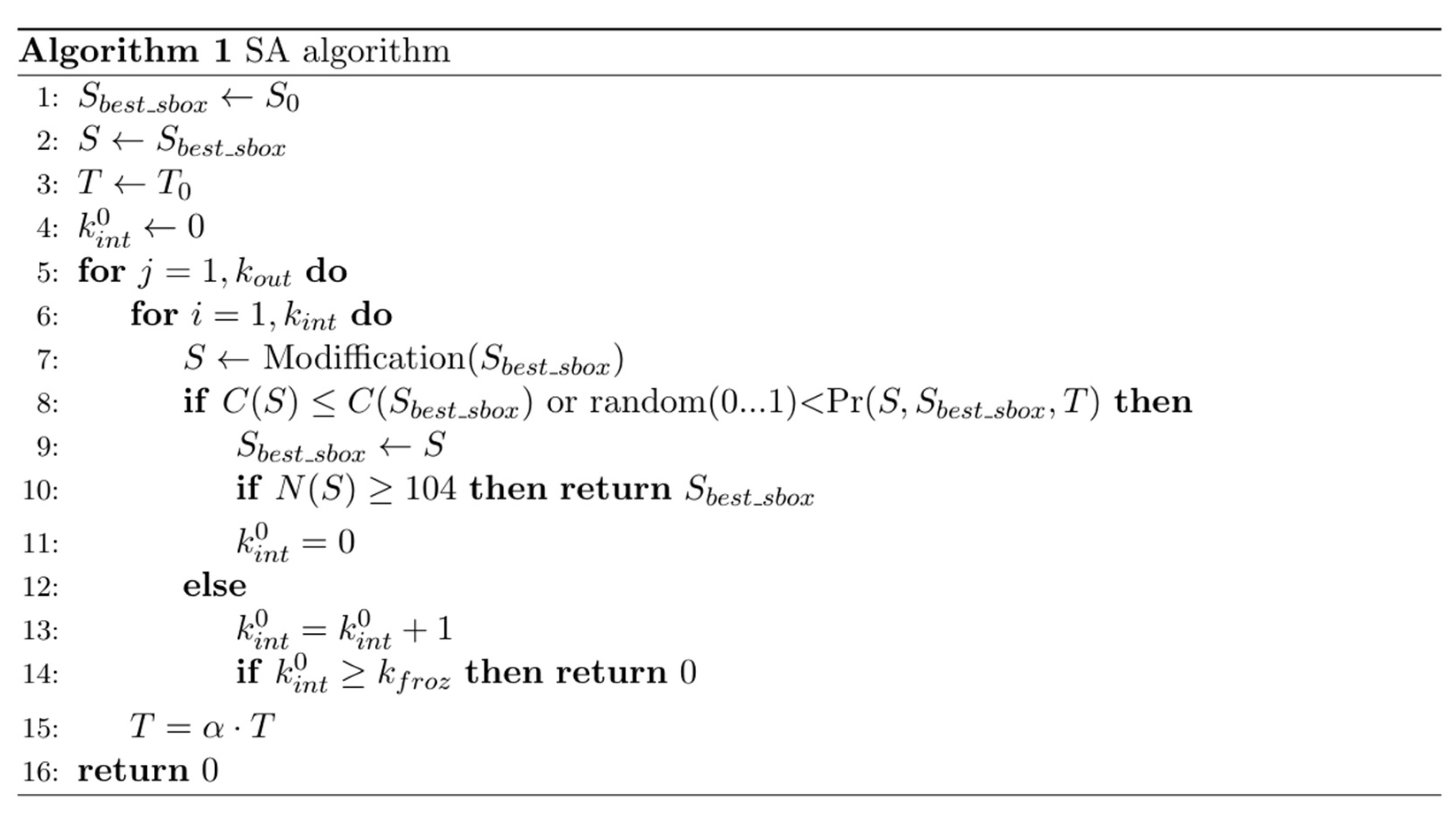
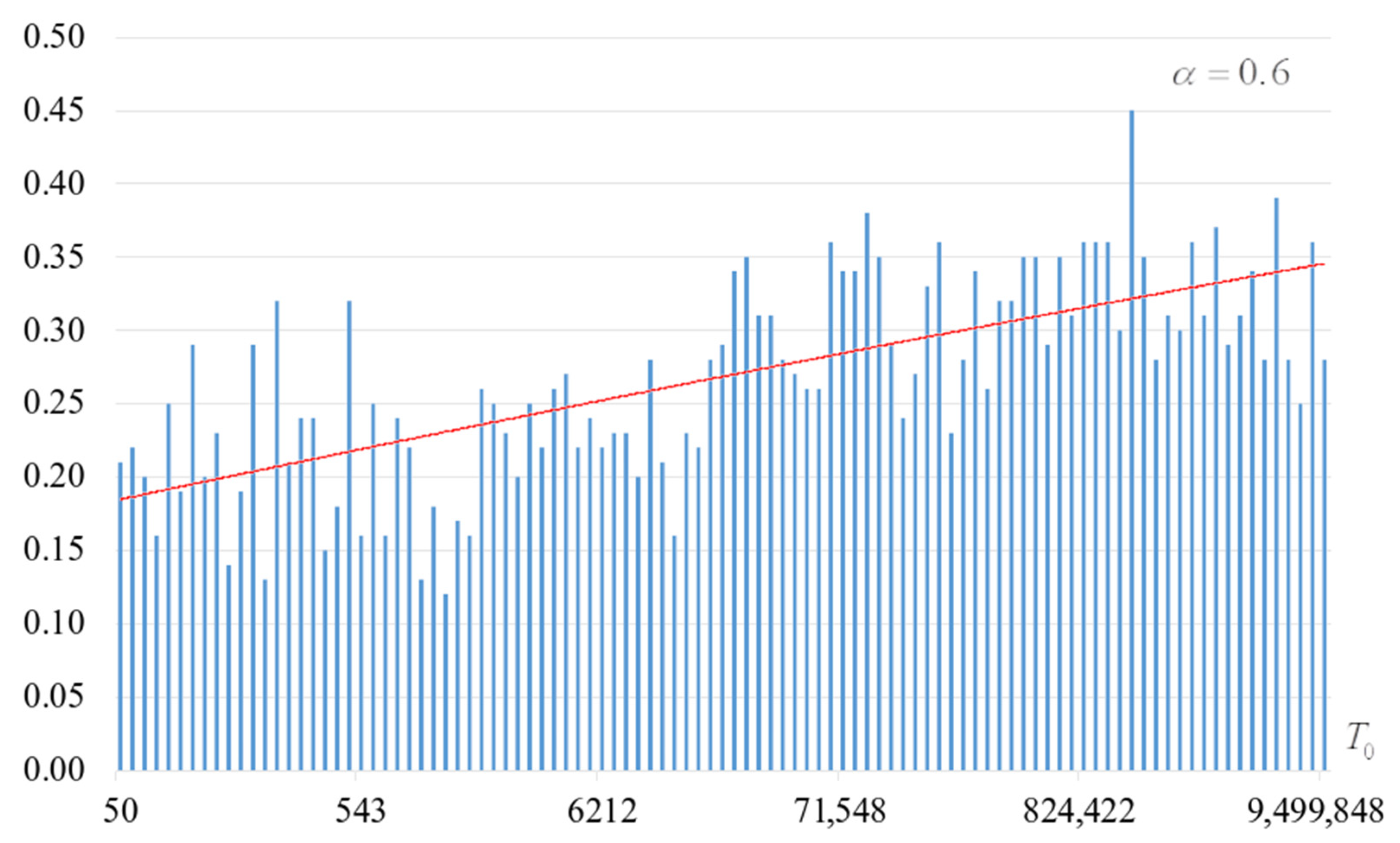
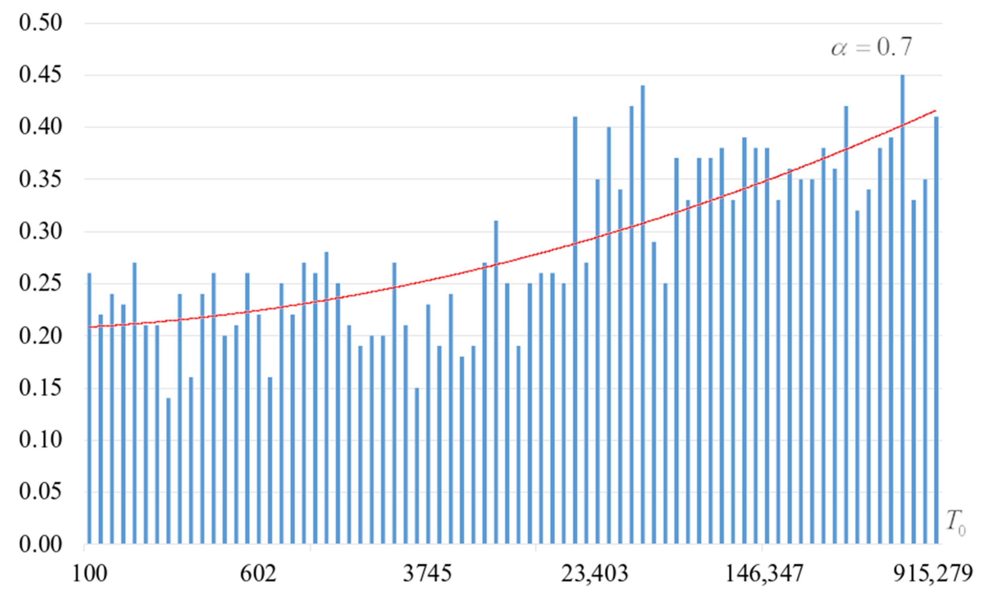
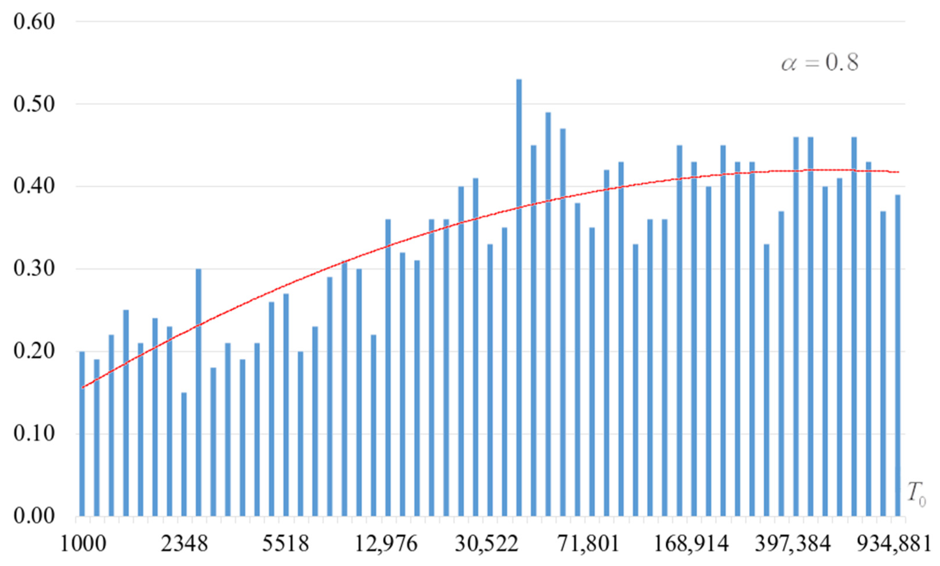
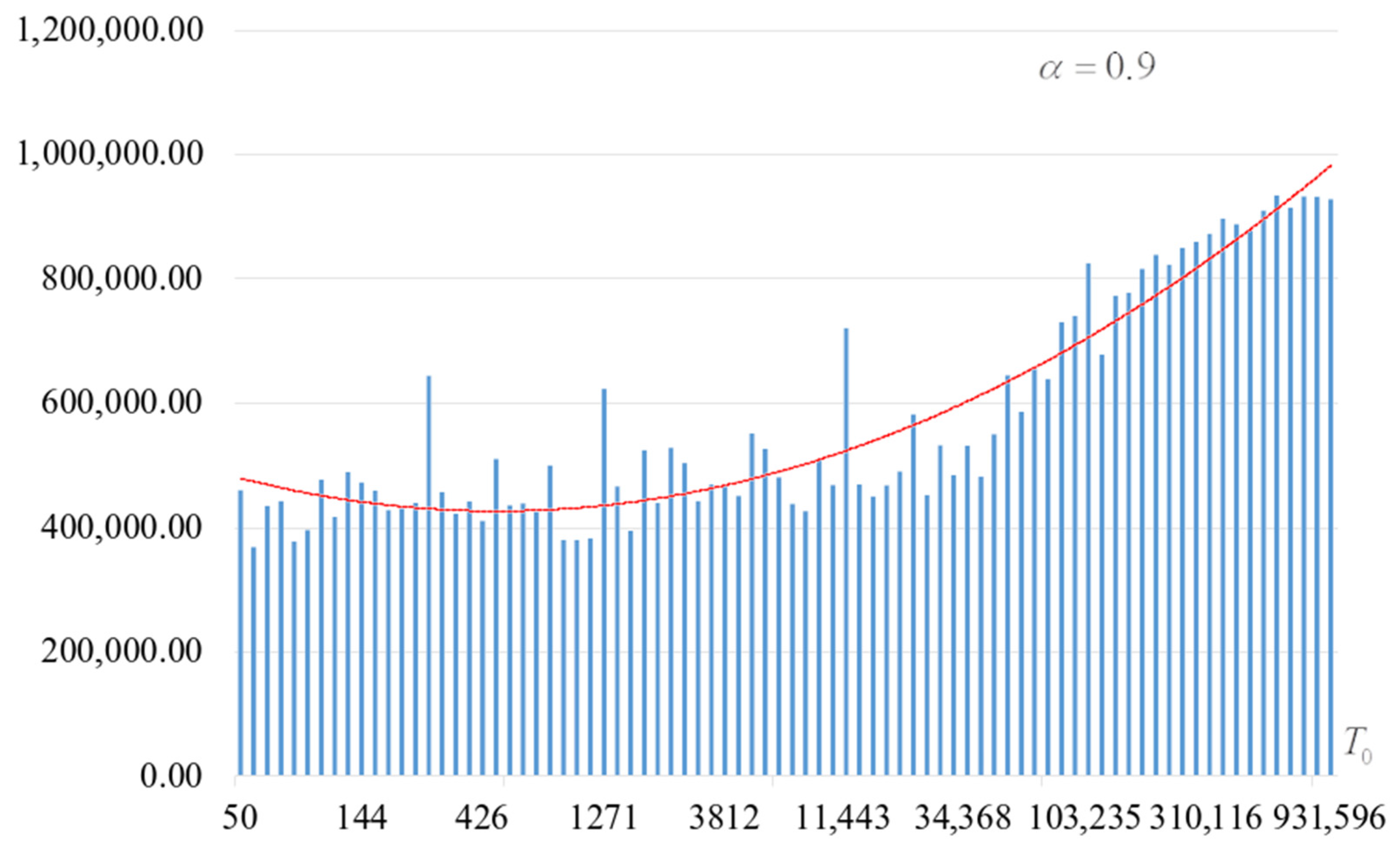
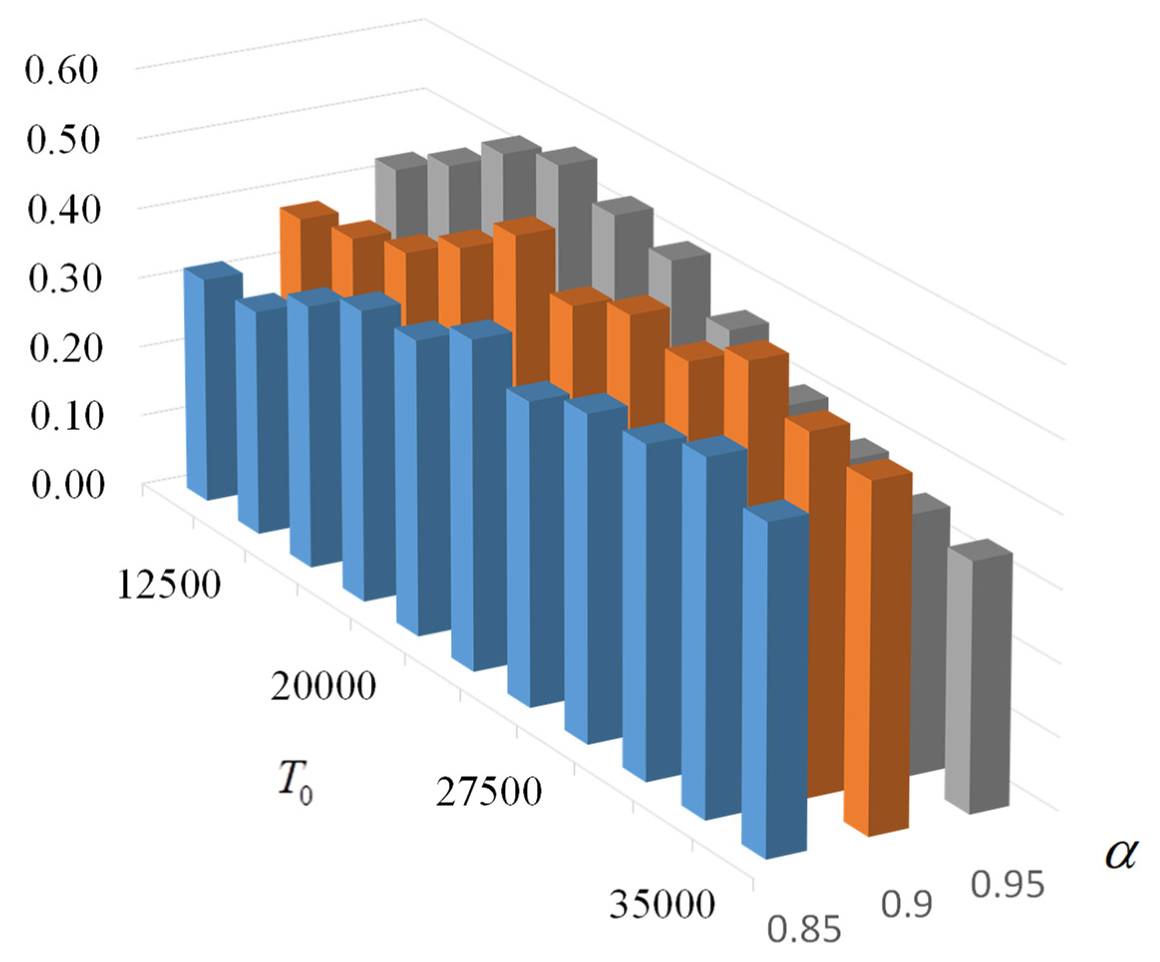
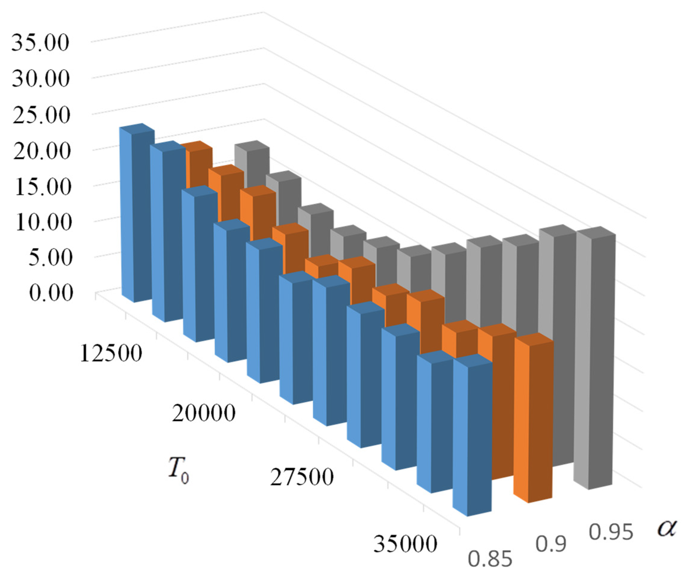
5. Results
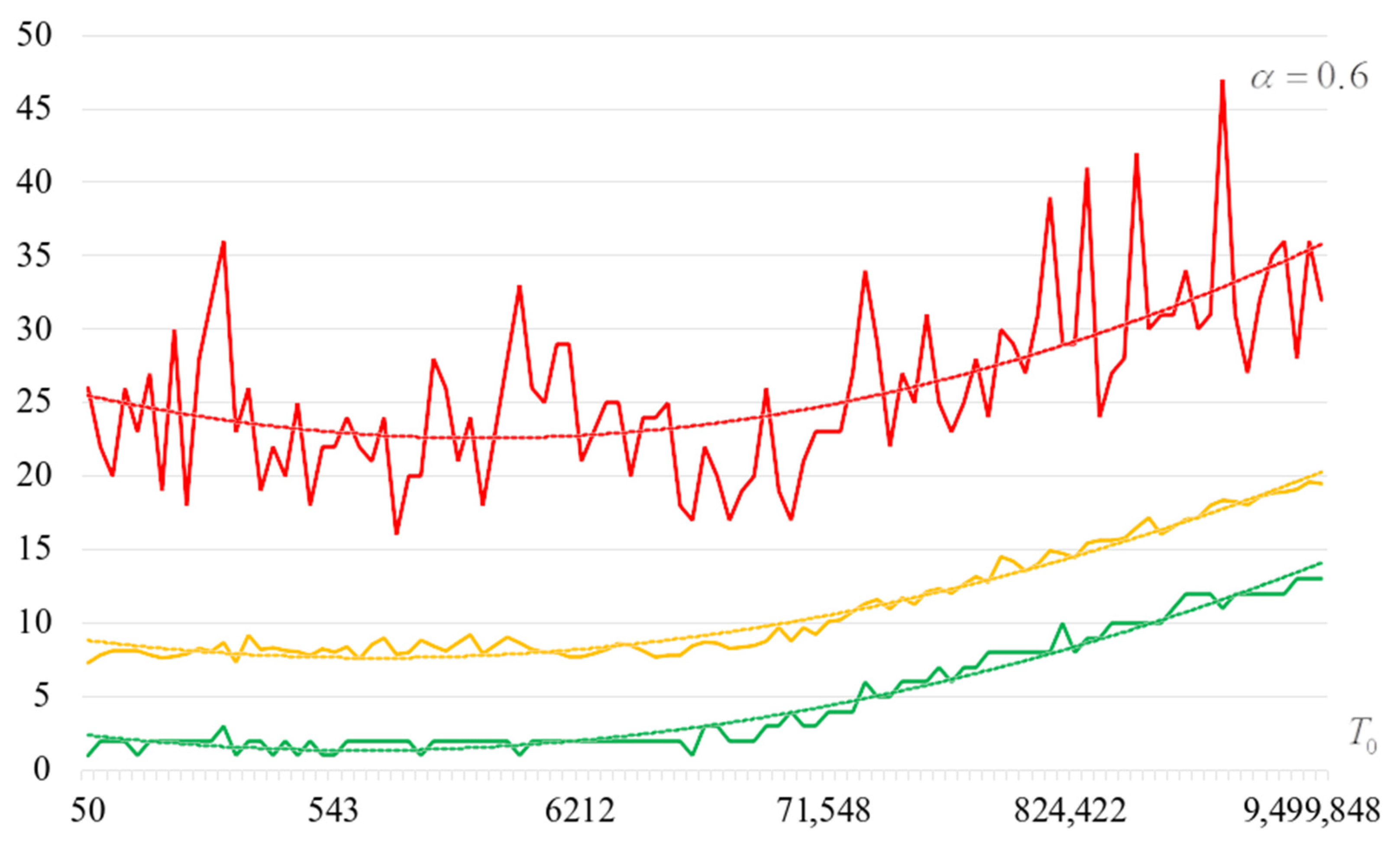
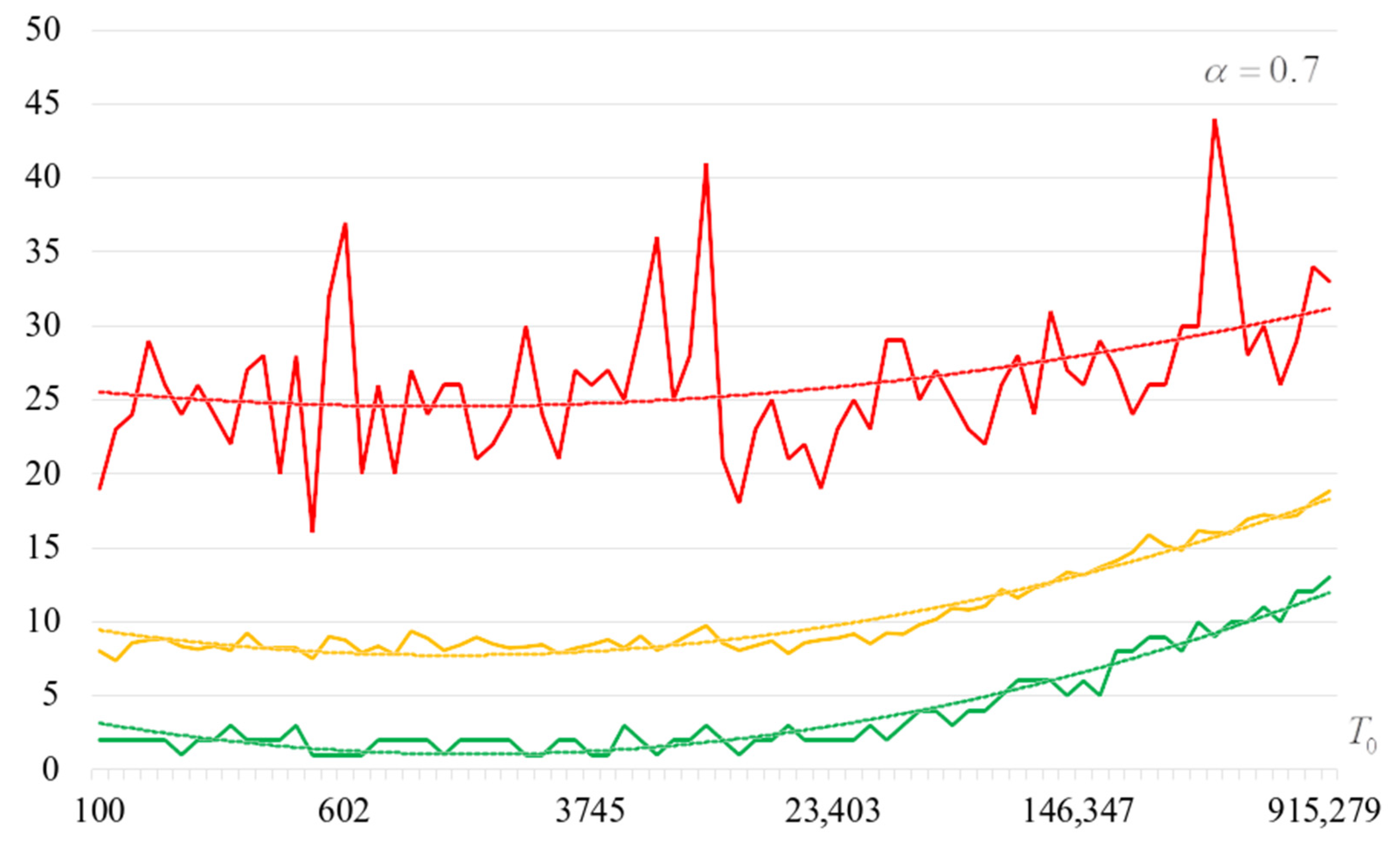
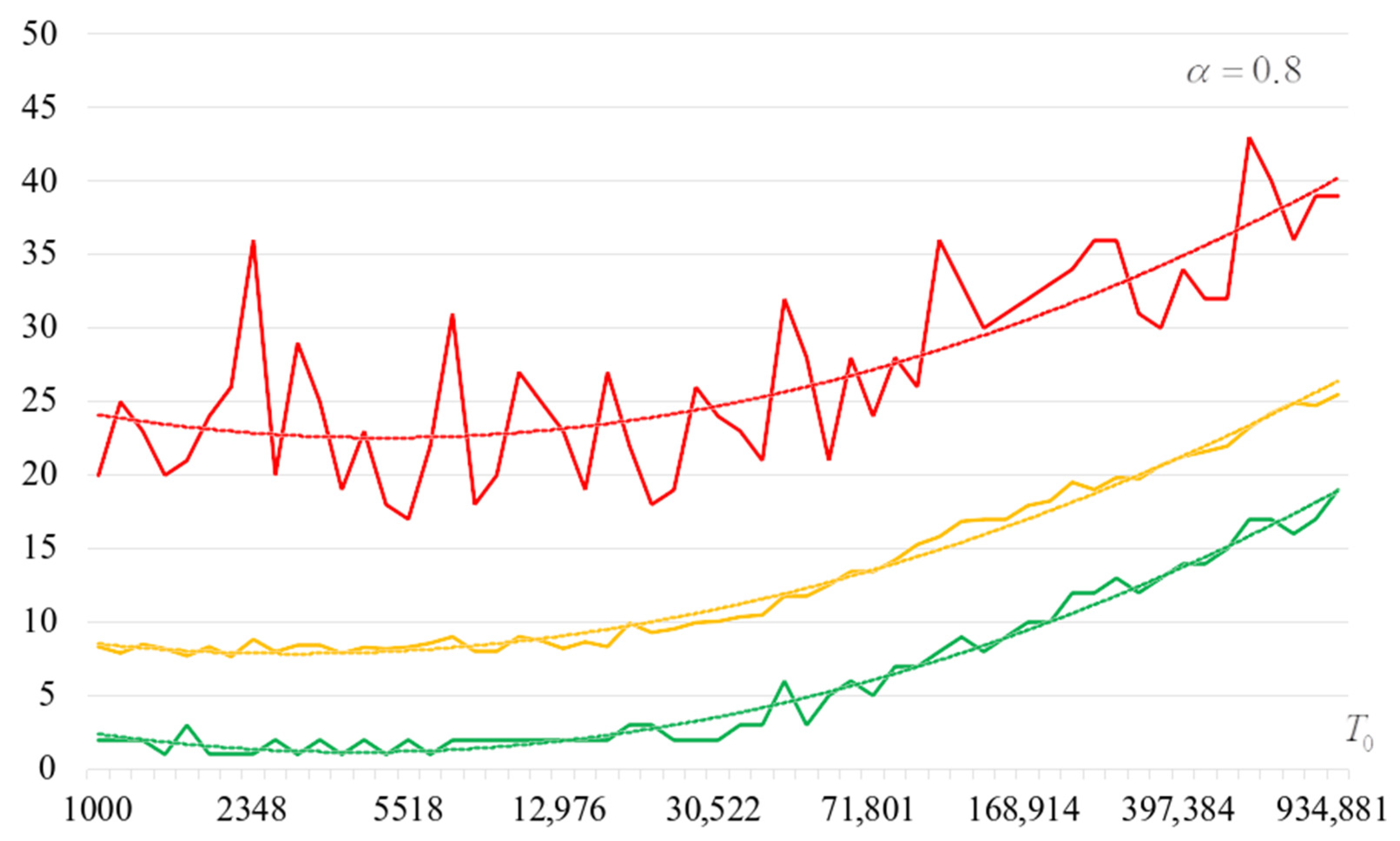
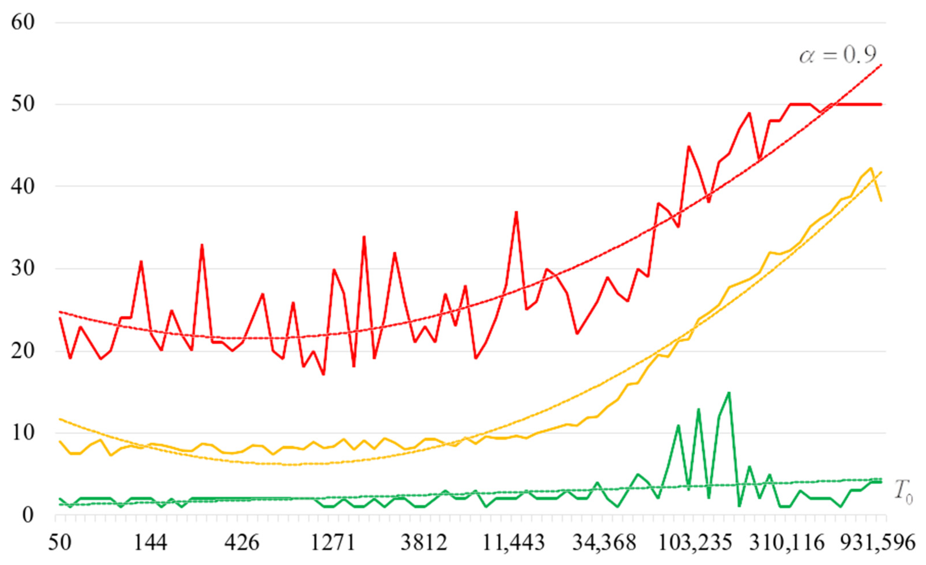
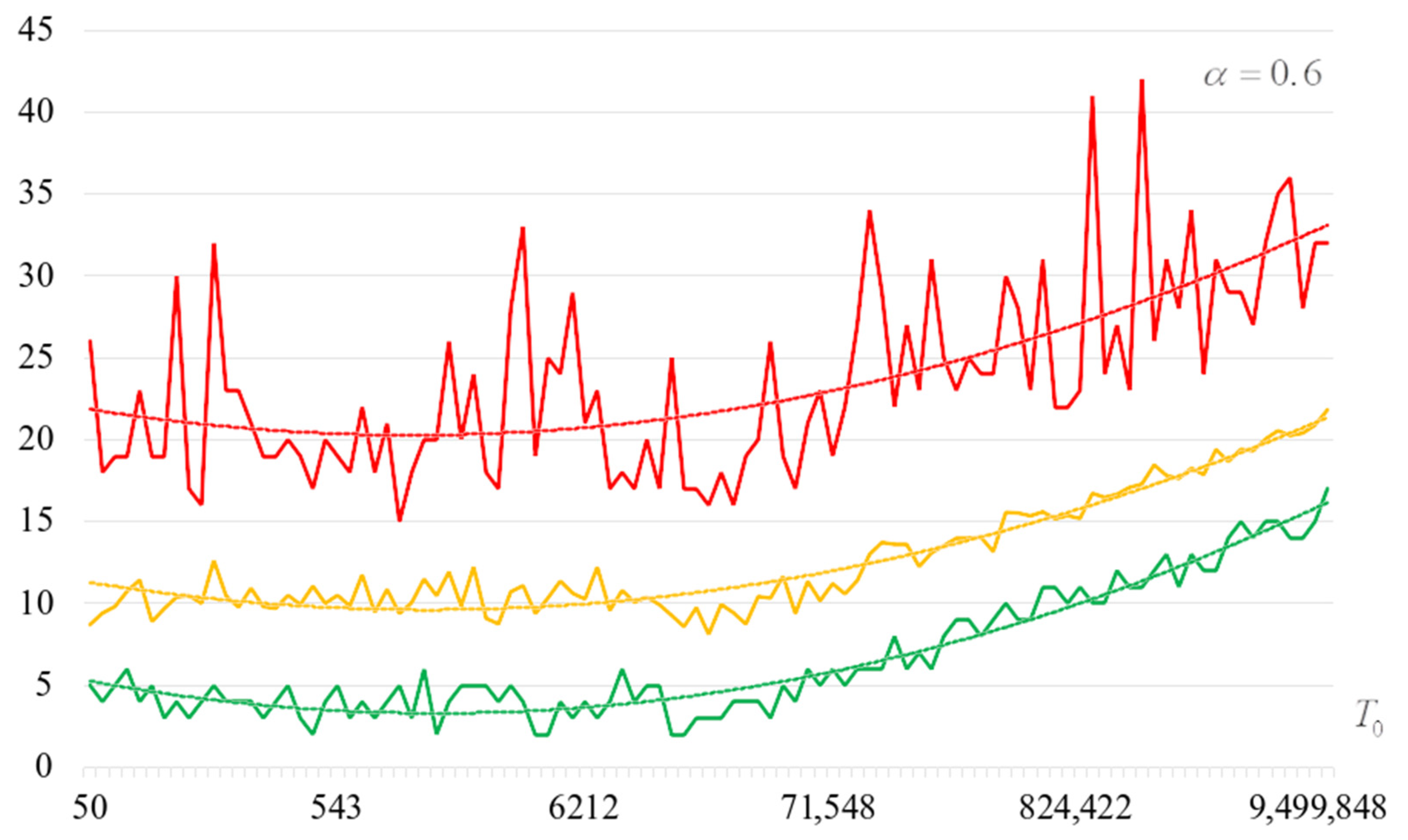
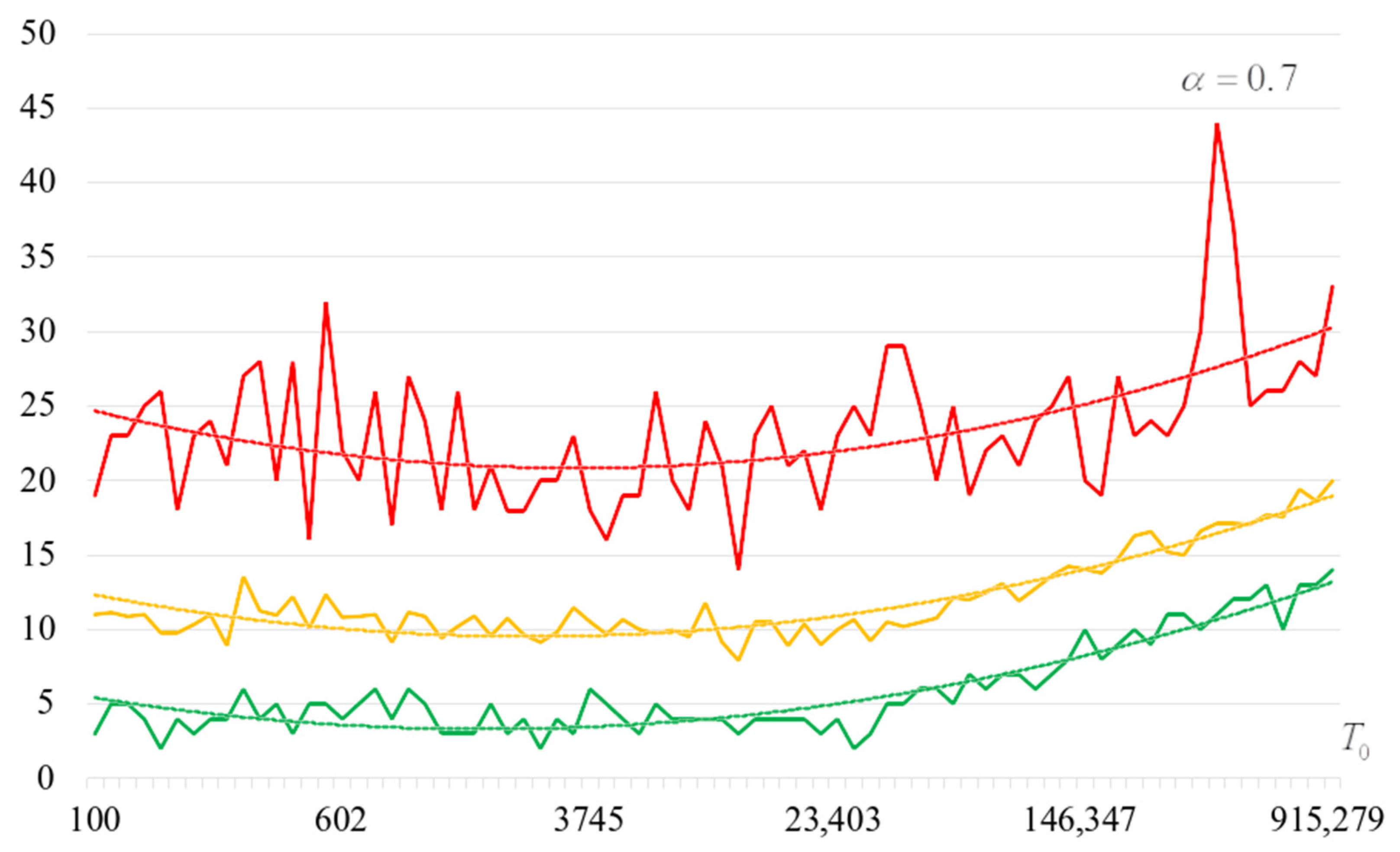
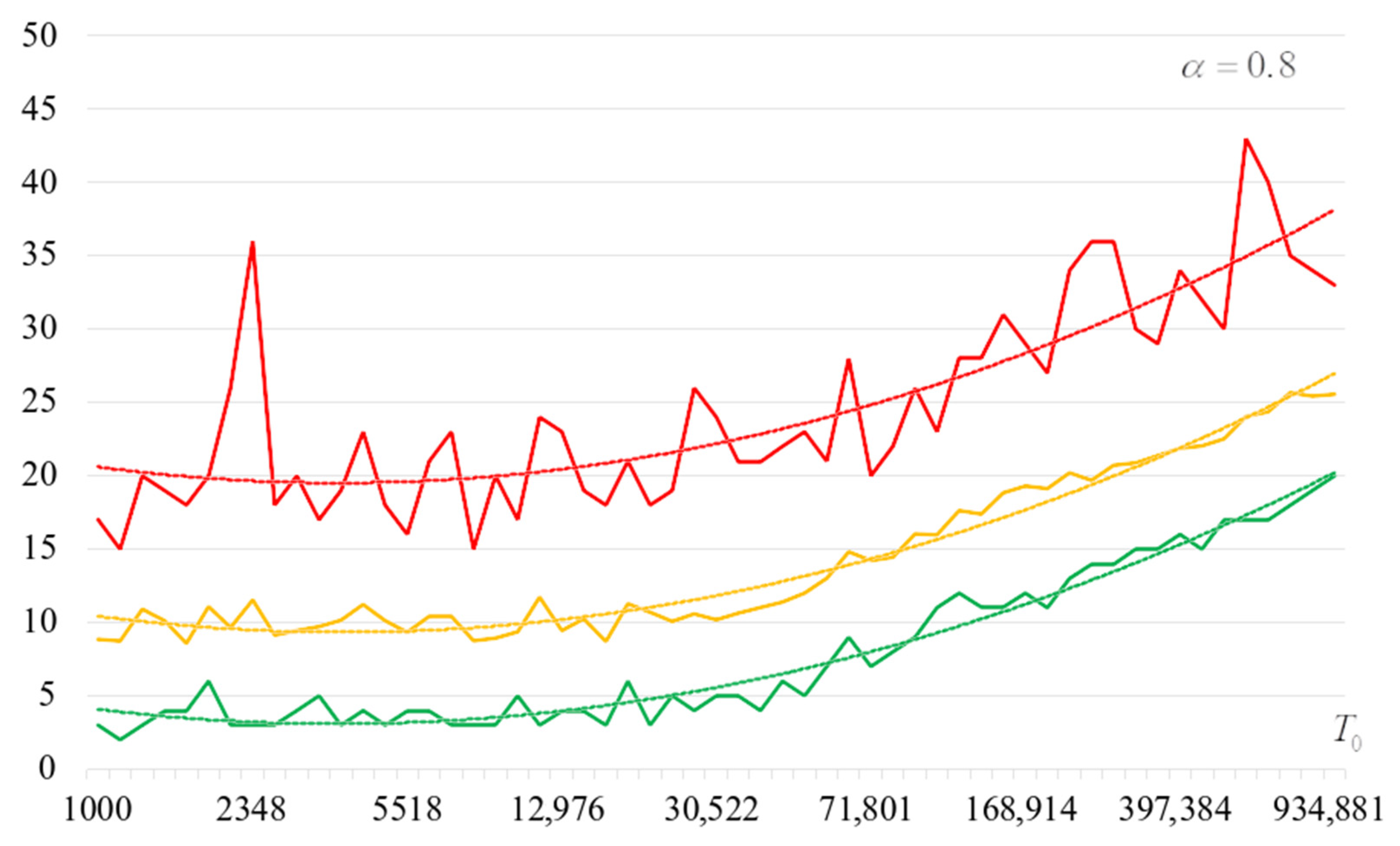
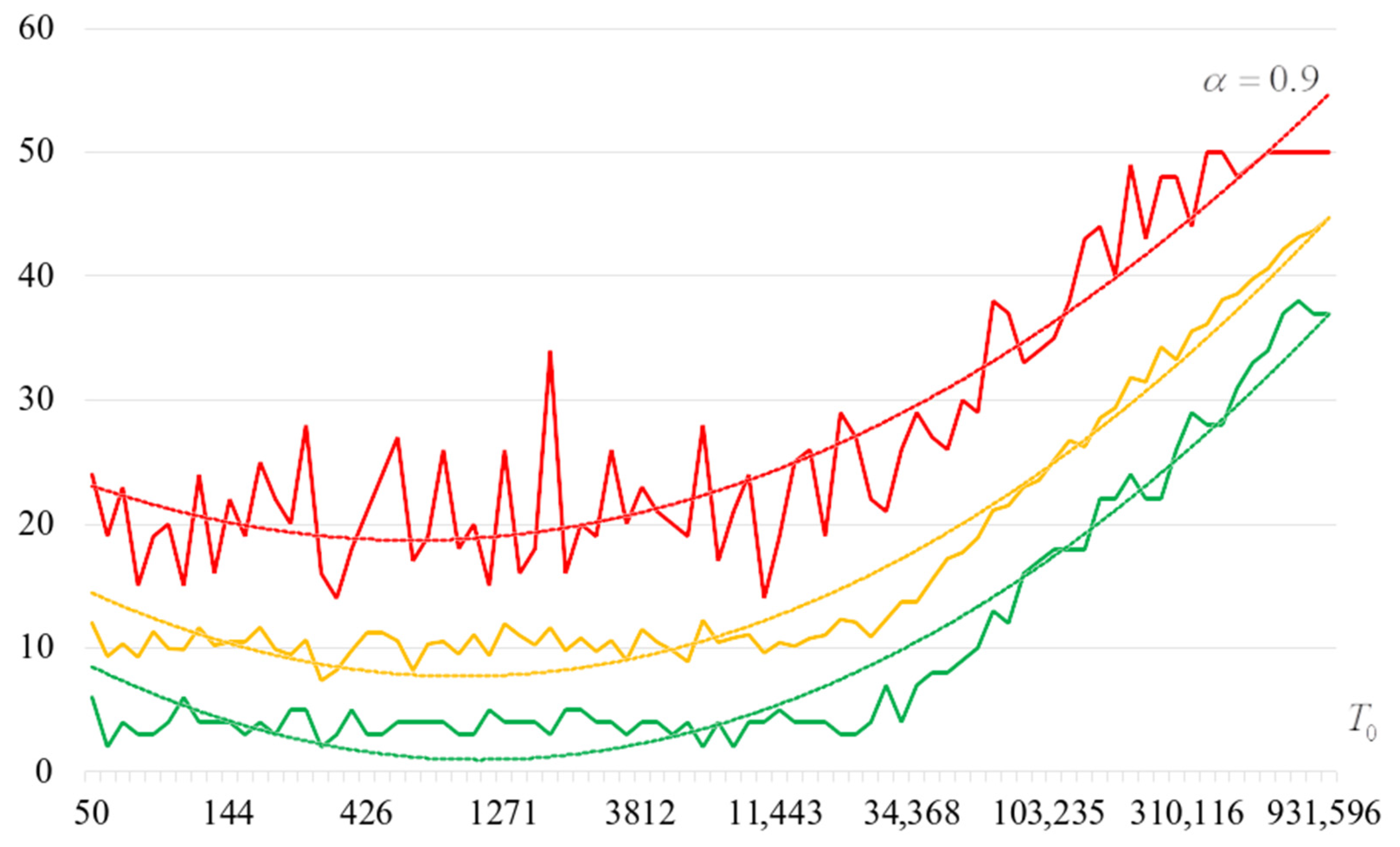
- The upper curve (red) corresponds to the maximum number of iterations;
- The middle curve (yellow) corresponds to the average number of iterations;
- The lower curve (green) corresponds to the minimum number of iterations.
- The upper curve (red) corresponds to the maximum number of iterations;
- The middle curve (yellow) corresponds to the average number of iterations;
- The lower curve (green) corresponds to the minimum number of iterations.
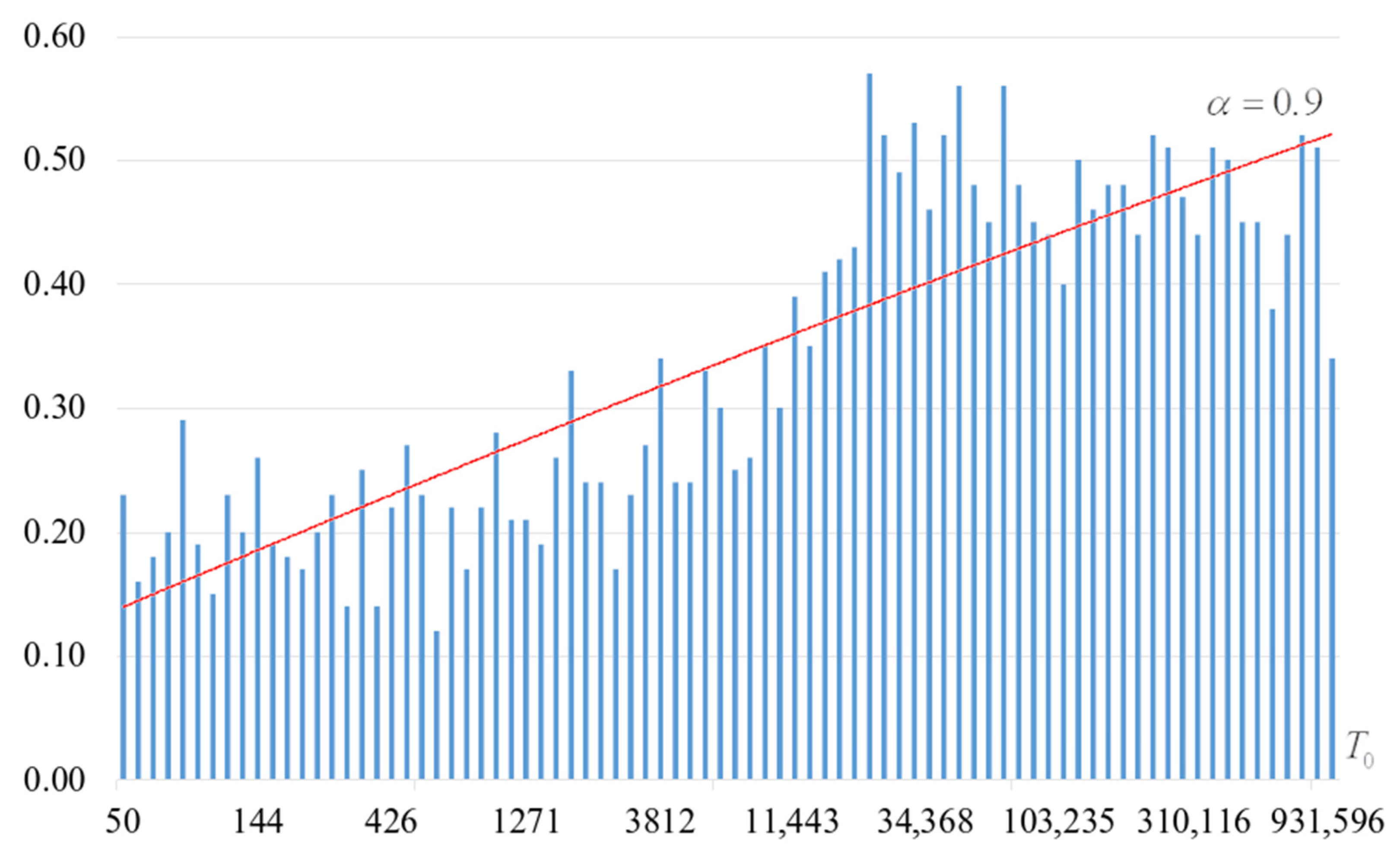
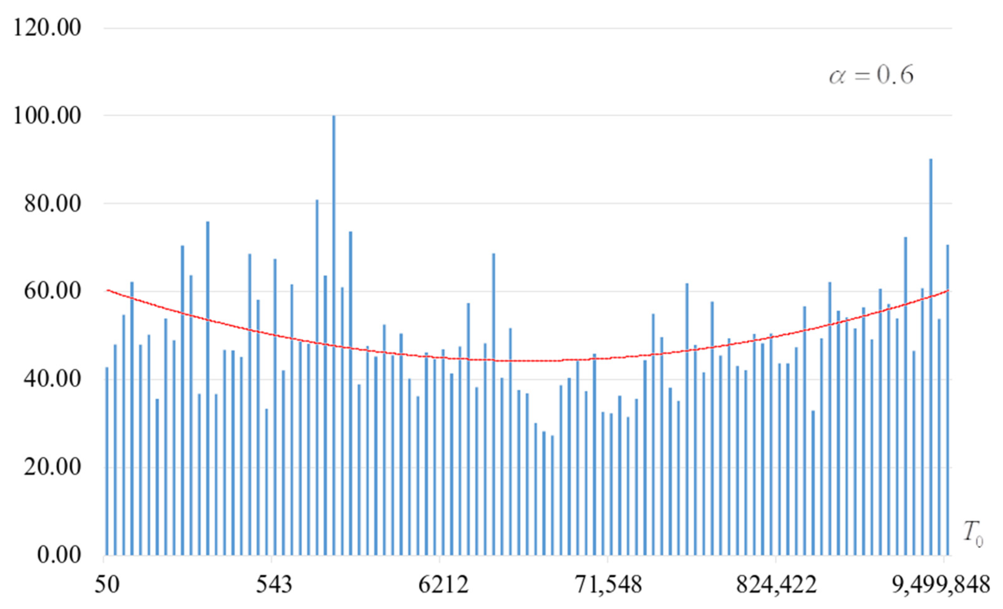
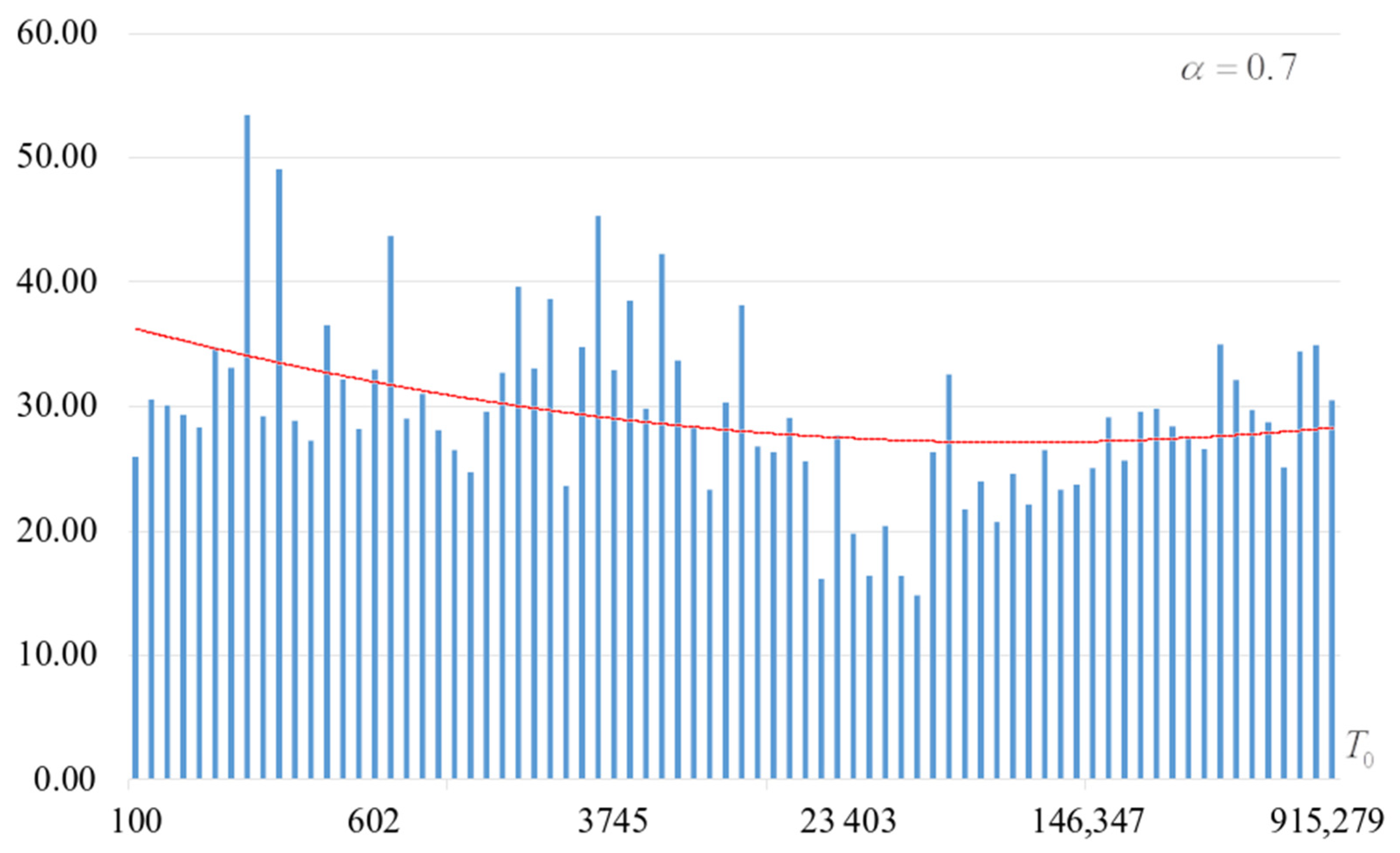
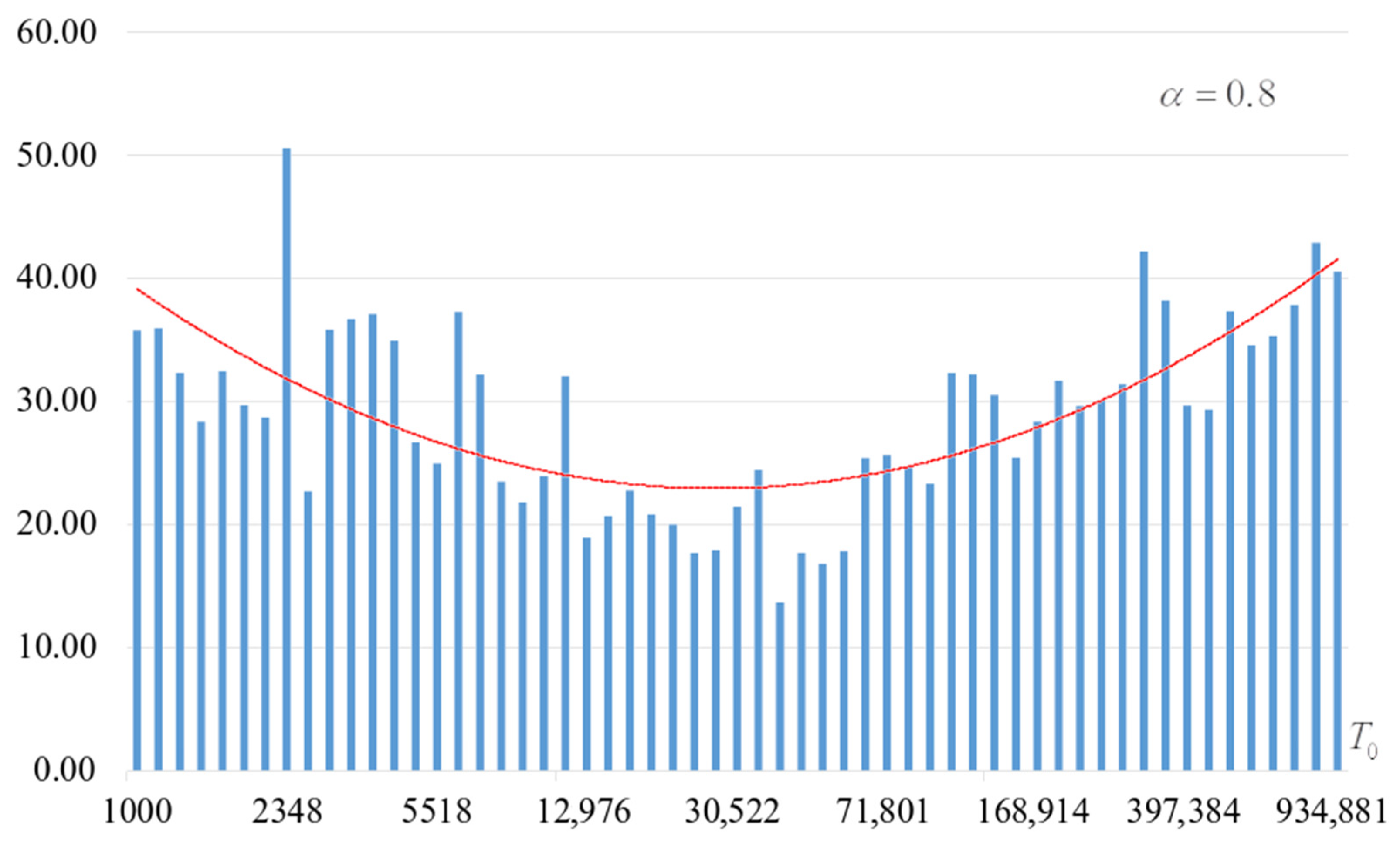
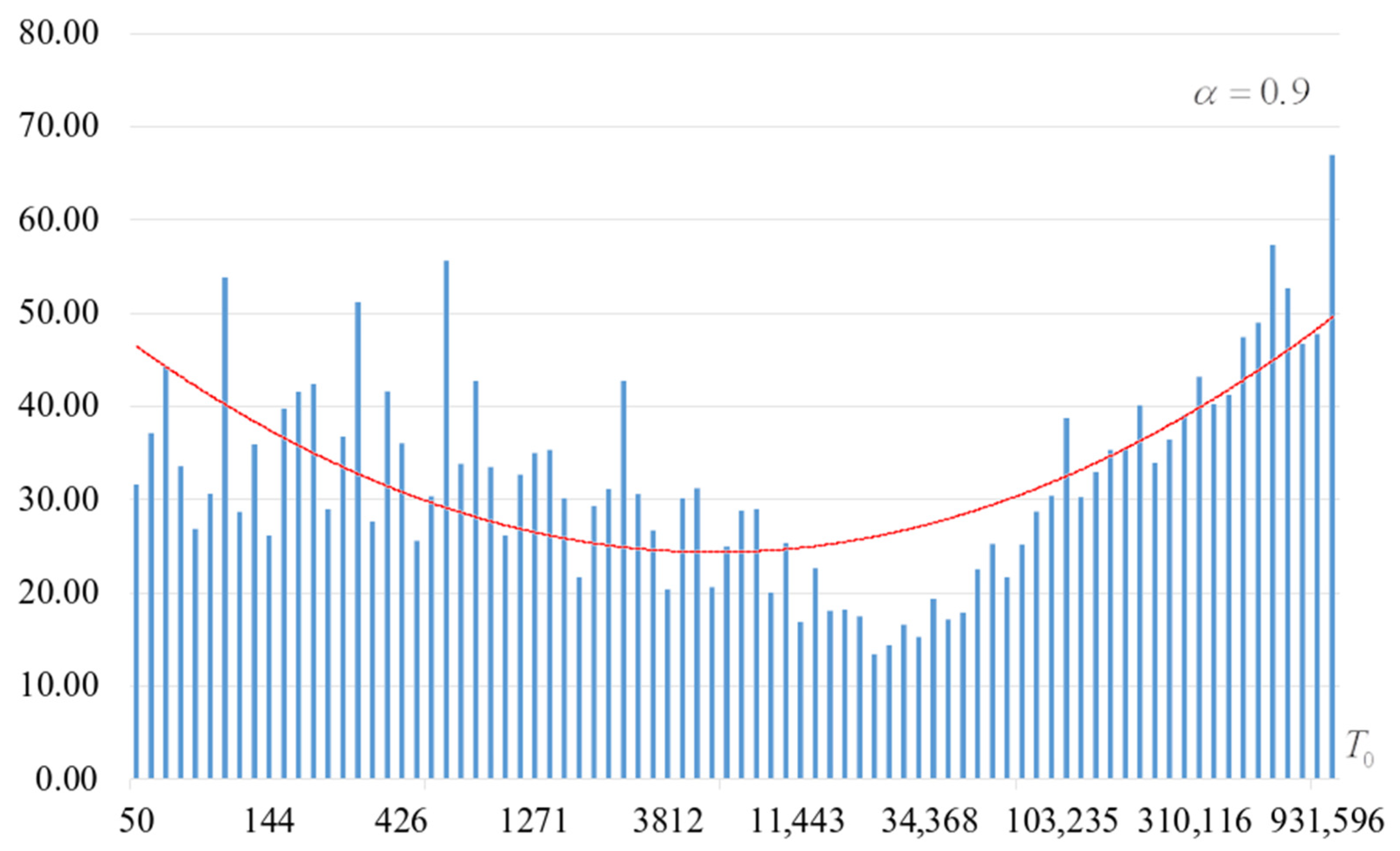
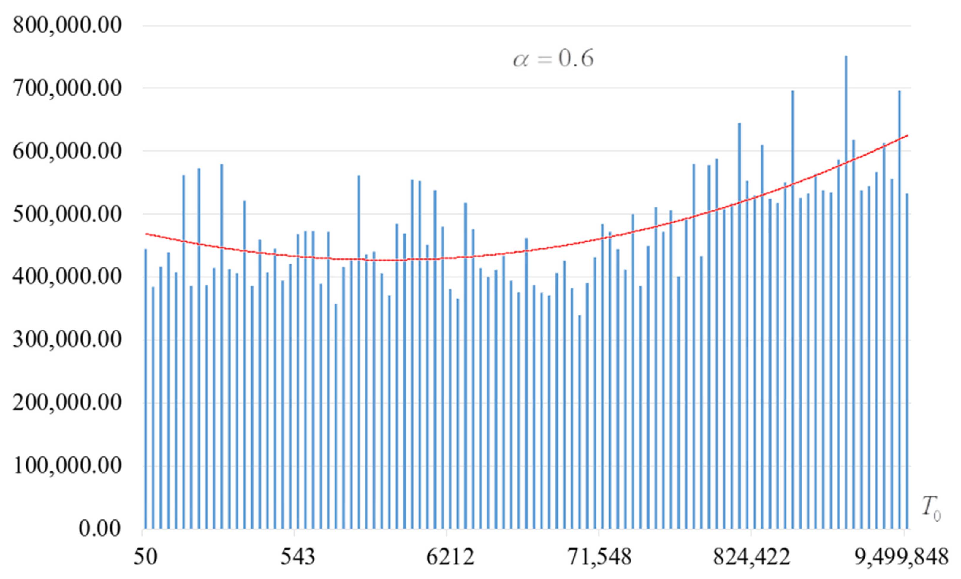
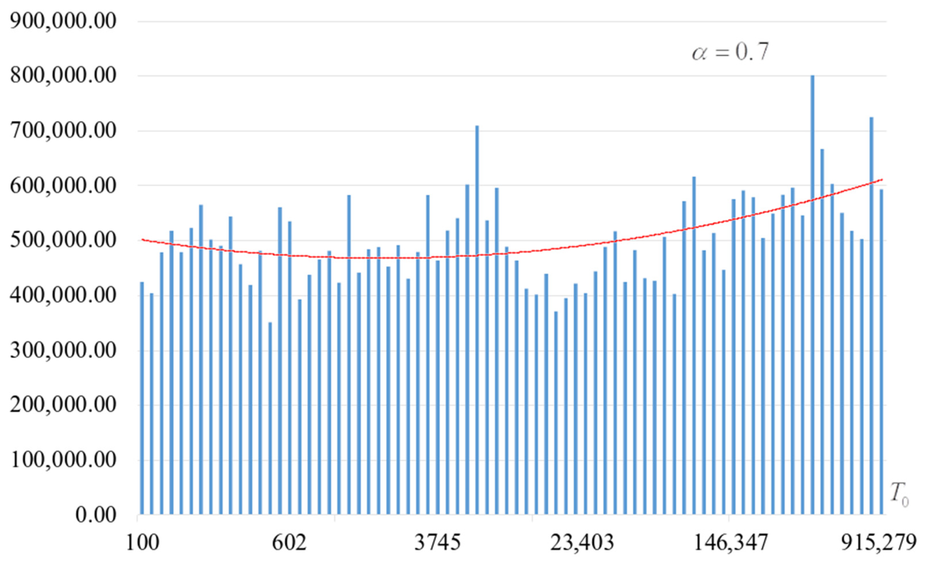
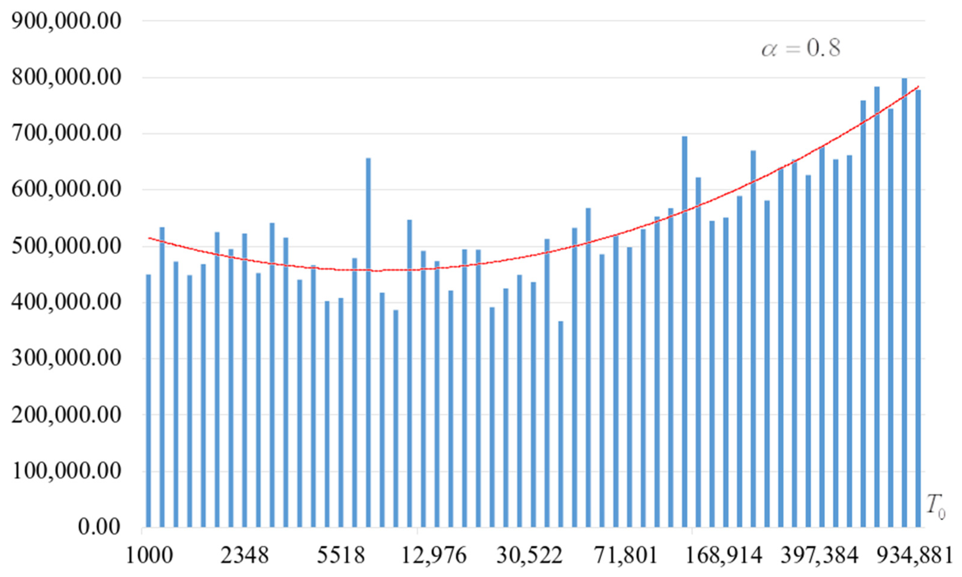
- As the value of grows, the total number of iterations is almost the same until a certain value (, depending on ) and then begins to grow rapidly, which causes a significant increase in the time to execute each run of the algorithm.
- If the is increased, the total number of search iterations decreases, i.e., substitution generation is performed faster.
6. Discussion
7. Conclusions
Author Contributions
Funding
Institutional Review Board Statement
Informed Consent Statement
Data Availability Statement
Conflicts of Interest
References
- Menezes, A.J.; van Oorschot, P.C.; Vanstone, S.A.; van Oorschot, P.C.; Vanstone, S.A. Handbook of Applied Cryptography; CRC Press: Boca Raton, FL, USA, 2018; ISBN 978-0-429-46633-5. [Google Scholar]
- Kuznetsov, A.A.; Potii, O.V.; Poluyanenko, N.A.; Gorbenko, Y.I.; Kryvinska, N. Stream Ciphers in Modern Real-Time IT Systems: Analysis, Design and Comparative Studies; Studies in Systems, Decision and Control; Springer International Publishing: New York, NY, USA, 2022; ISBN 978-3-030-79769-0. [Google Scholar]
- Kuznetsov, O.; Potii, O.; Perepelitsyn, A.; Ivanenko, D.; Poluyanenko, N. Lightweight Stream Ciphers for Green IT Engineering. In Green IT Engineering: Social, Business and Industrial Applications; Kharchenko, V., Kondratenko, Y., Kacprzyk, J., Eds.; Studies in Systems, Decision and Control; Springer International Publishing: Cham, Switzerland, 2019; Volume 171, pp. 113–137. ISBN 978-3-030-00252-7. [Google Scholar]
- Shannon, C.E. Communication Theory of Secrecy Systems. Bell Syst. Tech. J. 1949, 28, 656–715. [Google Scholar] [CrossRef]
- Rubinstein-Salzedo, S. Cryptography; Springer Undergraduate Mathematics Series; Springer International Publishing: Cham, Switzerland, 2018; ISBN 978-3-319-94817-1. [Google Scholar]
- Courtois, N.T.; Pieprzyk, J. Cryptanalysis of Block Ciphers with Overdefined Systems of Equations. In Advances in Cryptology—ASIACRYPT 2002; Zheng, Y., Ed.; Springer: Berlin/Heidelberg, Germany, 2002; pp. 267–287. [Google Scholar]
- Courtois, N.T.; Bard, G.V. Algebraic Cryptanalysis of the Data Encryption Standard. In Cryptography and Coding; Galbraith, S.D., Ed.; Springer: Berlin/Heidelberg, Germany, 2007; pp. 152–169. [Google Scholar]
- Daemen, J.; Rijmen, V. Specification of Rijndael. In The Design of Rijndael: The Advanced Encryption Standard (AES); Daemen, J., Rijmen, V., Eds.; Information Security and Cryptography; Springer: Berlin/Heidelberg, Germany, 2020; pp. 31–51. ISBN 978-3-662-60769-5. [Google Scholar]
- Bard, G.V. Algebraic Cryptanalysis; Springer US: Boston, MA, USA, 2009; ISBN 978-0-387-88756-2. [Google Scholar]
- Nover, H. Algebraic Cryptanalysis of Aes: An Overview; University of Wisconsin: Madison, WI, USA, 2005. [Google Scholar]
- Clark, J.A.; Jacob, J.L.; Stepney, S. The Design of S-Boxes by Simulated Annealing. In Proceedings of the 2004 Congress on Evolutionary Computation (IEEE Cat. No.04TH8753), Portland, OR, USA, 19–23 June 2004; Volume 2, pp. 1533–1537. [Google Scholar]
- McLaughlin, J.; Clark, J.A. Using Evolutionary Computation to Create Vectorial Boolean Functions with Low Differential Uniformity and High Nonlinearity. arXiv 2013, arXiv:1301.6972. [Google Scholar]
- Souravlias, D.; Parsopoulos, K.E.; Meletiou, G.C. Designing Bijective S-Boxes Using Algorithm Portfolios with Limited Time Budgets. Appl. Soft Comput. 2017, 59, 475–486. [Google Scholar] [CrossRef]
- Wang, J.; Zhu, Y.; Zhou, C.; Qi, Z. Construction Method and Performance Analysis of Chaotic S-Box Based on a Memorable Simulated Annealing Algorithm. Symmetry 2020, 12, 2115. [Google Scholar] [CrossRef]
- Delahaye, D.; Chaimatanan, S.; Mongeau, M. Simulated Annealing: From Basics to Applications; Springer: Berlin/Heidelberg, Germany, 2019; Volume 272, p. 1. ISBN 978-3-319-91086-4. [Google Scholar]
- Eremia, M.; Liu, C.-C.; Edris, A.-A. Heuristic Optimization Techniques. In Advanced Solutions in Power Systems: HVDC, FACTS, and Artificial Intelligence; IEEE: Piscataway, NJ, USA, 2016; pp. 931–984. ISBN 978-1-119-17533-9. [Google Scholar]
- Beth, T.; Ding, C. On Almost Perfect Nonlinear Permutations. In Advances in Cryptology—EUROCRYPT ’93; Helleseth, T., Ed.; Springer: Berlin/Heidelberg, Germany, 1994; pp. 65–76. [Google Scholar]
- Nyberg, K. Differentially Uniform Mappings for Cryptography. In Advances in Cryptology—EUROCRYPT ’93; Helleseth, T., Ed.; Springer: Berlin/Heidelberg, Germany, 1994; pp. 55–64. [Google Scholar]
- Clark, A.J. Optimisation Heuristics for Cryptology. Ph.D. Thesis, Queensland University of Technology, Brisbane, Australia, 1998. [Google Scholar]
- Kose, U.; Kose, U.; Guraksin, G.E.; Deperlioglu, O. (Eds.) Nature-Inspired Intelligent Techniques for Solving Biomedical Engineering Problems; Advances in Bioinformatics and Biomedical Engineering; IGI Global: Hershey, PA, USA, 2018; ISBN 978-1-5225-4769-3. [Google Scholar]
- Information Resources Management Association. Nature-Inspired Computing: Concepts, Methodologies, Tools, and Applications; IGI Global: Hershey, PA, USA, 2017; ISBN 978-1-5225-0788-8. [Google Scholar]
- Korte, B.; Vygen, J. Combinatorial Optimization: Theory and Algorithms, 6th ed.; Springer: Berlin/Heidelberg, Germany, 2018. [Google Scholar]
- Oliva, D.; Houssein, E.H.; Hinojosa, S. (Eds.) Metaheuristics in Machine Learning: Theory and Applications; Studies in Computational Intelligence; Springer International Publishing: Cham, Switzerland, 2021; Volume 967, ISBN 978-3-030-70541-1. [Google Scholar]
- Zamani, H.; Nadimi-Shahraki, M.H.; Gandomi, A.H. Starling Murmuration Optimizer: A Novel Bio-Inspired Algorithm for Global and Engineering Optimization. Comput. Methods Appl. Mech. Eng. 2022, 392, 114616. [Google Scholar] [CrossRef]
- Li, Y.; Carabelli, S.; Fadda, E.; Manerba, D.; Tadei, R.; Terzo, O. Machine Learning and Optimization for Production Rescheduling in Industry 4.0. Int. J. Adv. Manuf. Technol. 2020, 110, 2445–2463. [Google Scholar] [CrossRef]
- Zamani, H.; Nadimi-Shahraki, M.H.; Gandomi, A.H. QANA: Quantum-Based Avian Navigation Optimizer Algorithm. Eng. Appl. Artif. Intell. 2021, 104, 104314. [Google Scholar] [CrossRef]
- Yu, V.F.; Susanto, H.; Jodiawan, P.; Ho, T.-W.; Lin, S.-W.; Huang, Y.-T. A Simulated Annealing Algorithm for the Vehicle Routing Problem With Parcel Lockers. IEEE Access 2022, 10, 20764–20782. [Google Scholar] [CrossRef]
- Tang, O. Simulated Annealing in Lot Sizing Problems. Int. J. Prod. Econ. 2004, 88, 173–181. [Google Scholar] [CrossRef]
- Tesar, P. A New Method for Generating High Non-Linearity S-Boxes. Radioengineering 2010, 19, 23–26. [Google Scholar]
- Picek, S.; Cupic, M.; Rotim, L. A New Cost Function for Evolution of S-Boxes. Evol. Comput. Winter 2016, 24, 695–718. [Google Scholar] [CrossRef] [PubMed]
- Freyre-Echevarría, A.; Alanezi, A.; Martínez-Díaz, I.; Ahmad, M.; Abd El-Latif, A.A.; Kolivand, H.; Razaq, A. An External Parameter Independent Novel Cost Function for Evolving Bijective Substitution-Boxes. Symmetry 2020, 12, 1896. [Google Scholar] [CrossRef]
- Freyre Echevarría, A.; Martínez Díaz, I. A New Cost Function to Improve Nonlinearity of Bijective S-Boxes. 2020; preprint. [Google Scholar]
- Kuznetsov, A.; Poluyanenko, N.; Kandii, S.; Zaichenko, Y.; Prokopovich-Tkachenko, D.; Katkova, T. WHS Cost Function for Generating S-Boxes. In Proceedings of the 2021 IEEE 8th International Conference on Problems of Infocommunications, Science and Technology (PIC S&T), Kharkiv, Ukraine, 5–7 October 2021; pp. 434–438. [Google Scholar]
- Chen, G. A Novel Heuristic Method for Obtaining S-Boxes. Chaos Solitons Fractals 2008, 36, 1028–1036. [Google Scholar] [CrossRef]
- Kuznetsov, A.; Poluyanenko, N.; Kandii, S.; Zaichenko, Y.; Prokopovich-Tkachenko, D.; Katkova, T. Optimizing the Local Search Algorithm for Generating S-Boxes. In Proceedings of the 2021 IEEE 8th International Conference on Problems of Infocommunications, Science and Technology (PIC S&T), Kharkiv, Ukraine, 5–7 October 2021; pp. 458–464. [Google Scholar]
- McLaughlin, J. Applications of Search Techniques to Cryptanalysis and the Construction of Cipher Components. Ph.D. Thesis, University of York, Heslington, UK, 2012. [Google Scholar]
- Ivanov, G.; Nikolov, N.; Nikova, S. Cryptographically Strong S-Boxes Generated by Modified Immune Algorithm. In Cryptography and Information Security in the Balkans; Pasalic, E., Knudsen, L.R., Eds.; Springer International Publishing: Cham, Switzerland, 2016; pp. 31–42. [Google Scholar]


| The Number of External Loops of the Algorithm for Which No Improvement of the Cost Function Was Found | ||||||||||||
|---|---|---|---|---|---|---|---|---|---|---|---|---|
| 0 | 1 | 2 | 3 | 4 | 5 | |||||||
| 0.6 | 4281 | 42% | 3042 | 30% | 1509 | 15% | 725 | 7% | 402 | 4% | 141 | 1.4% |
| 0.7 | 2722 | 36% | 2510 | 33% | 1245 | 16% | 641 | 8% | 355 | 5% | 127 | 1.7% |
| 0.8 | 1362 | 24% | 2060 | 36% | 1244 | 22% | 592 | 10% | 322 | 6% | 120 | 2.1% |
| 0.9 | 2168 | 26% | 1671 | 20% | 1634 | 20% | 1466 | 18% | 955 | 12% | 306 | 3.7% |
| 0.95 | 2299 | 28% | 1684 | 21% | 1333 | 16% | 1163 | 14% | 1167 | 14% | 554 | 6.8% |
| SA [11], SA [37] | SA [14] | SA [12] | Our Work | |
|---|---|---|---|---|
| The highest value of obtained in the found S-box | 102 | 92 | 104 | 104 |
| S-box generation probability | 1/200 = 0.5% | - | - | 56.4% |
| S-box generation (search) time | - | - | - | 14.2 s |
| Generation complexity (number of search iterations) | - | - | 3,000,000 30,000,000 | 450,000 |
Publisher’s Note: MDPI stays neutral with regard to jurisdictional claims in published maps and institutional affiliations. |
© 2022 by the authors. Licensee MDPI, Basel, Switzerland. This article is an open access article distributed under the terms and conditions of the Creative Commons Attribution (CC BY) license (https://creativecommons.org/licenses/by/4.0/).
Share and Cite
Kuznetsov, A.; Wieclaw, L.; Poluyanenko, N.; Hamera, L.; Kandiy, S.; Lohachova, Y. Optimization of a Simulated Annealing Algorithm for S-Boxes Generating. Sensors 2022, 22, 6073. https://doi.org/10.3390/s22166073
Kuznetsov A, Wieclaw L, Poluyanenko N, Hamera L, Kandiy S, Lohachova Y. Optimization of a Simulated Annealing Algorithm for S-Boxes Generating. Sensors. 2022; 22(16):6073. https://doi.org/10.3390/s22166073
Chicago/Turabian StyleKuznetsov, Alexandr, Lukasz Wieclaw, Nikolay Poluyanenko, Lukasz Hamera, Sergey Kandiy, and Yelyzaveta Lohachova. 2022. "Optimization of a Simulated Annealing Algorithm for S-Boxes Generating" Sensors 22, no. 16: 6073. https://doi.org/10.3390/s22166073