
Towards an Explainable Universal Feature Set for IoT Intrusion Detection


Abstract
:1. Introduction
- The focus of many IoT manufacturers is around optimal efficiency in production, and overlook security concerns in the devices they produce. According to [4], many manufacturers utilize outdated open-source firmware with many known vulnerabilities without any patching or security testing;
- On rare occasions that manufacturers issue patches, these patches are usually difficult to apply, and non-technical users face difficulties in applying them and end up not applying them successfully. Most of the used firmware does not support Over-The-Air (OTA) updates, and this makes the pathcing process very challenging and error prone;
- IoT devices are known to be resource-constrained. The available memory and processing power are usually limited and barely adequate for the devices to do its job.This makes them hard to defend at the host-level;
- Many IoT device users do not change the default settings. This means that many devices use their default usernames and passwords that can easily be guessed or brute-forced, as in the case of the Mirai botnet [5]. In certain cases, these credentials are hard-coded into the firmware and cannot be changed by users.
1.1. Research Contribution
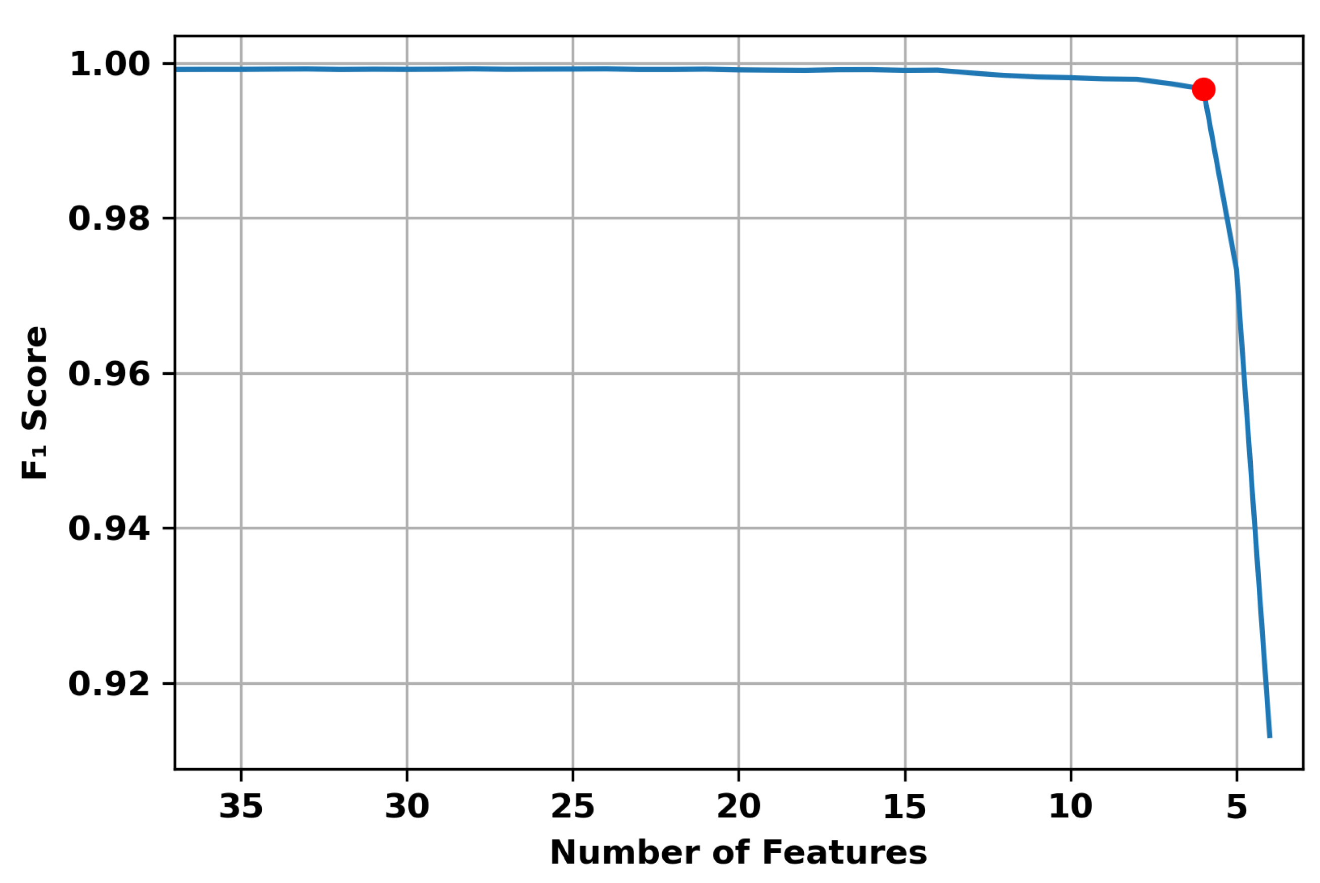
- Reduce the number of features needed to create a high-accuracy intrusion detection model. The selected features were only six flow-based network features;
- Achieve an accuracy of 99.62% in the testing of the trained machine learning classifier dataset;
- Explain the selected features using SHAP values to provide a better understanding of how the model makes a prediction;
- Create a smaller version of the TON_IoT dataset that can be used in real-life implementations of machine learning-based IoT IDS.
1.2. Paper Layout
2. Related Works
3. The Dataset
- Raw datasetsCollected from 10 IoT and IIoT sensors, network capture (pcap), Linux tracing tool dataset, and Windows collectors of the Performance Monitor Tool on Windows 7 and 10 systems;
- Processed datasets;
- Train-Test-datasets.
- Man-In-The-Middle (MITM) ARP Spoofing;
- Denial of Service attack (SYN flooding);
- Mirai botnet (UDP flooding, ACK flooding, HTTP flooding, host discovery, telnet brute-force);
- Port and Operating System (OS) scanning;
- Host scanning.
4. Preprocessing
4.1. Classifier Selection
- Random Forest;
- Logistic Regression (LR);
- Decision Tree (DT);
- Gaussian Naive-Bayes (GNB).
4.2. Dataset Observations and Preprocessing Steps for TON_IoT
- Missing values were replaced with a ‘-’;
- MITM attack category represented only 0.22% of the dataset;
- Several data fields included non-numerical values, such as source and destination IP addresses, protocol, and service types;
- There were features that logically do not impact the predictions, such as timestamp;
- The “malicious” and “benign” labels are reasonably balanced with 300,000 benign instances, and 161,043 malicious instances;
- The dataset includes features that are host-specific such as the src_ip and dst_ip.
| Algorithm 1: TON_IoT Dataset Proprocessing |
| Input: TON_IoT train-test Dataset (461,043 instances, 45 features) Output: Balanced Dataset with no missing data (461,043 instance, 37 features) In () remove label In () remove features In () remove features label-encode |
4.3. Observations and Preprocessing Steps for IoT-ID
- The original pcap files were split into benign and malicious pcap files according to the information provided with the dataset;
- The CSV files were combined into a single dataset containing 20 features, including the 6 feature that were selected in our experiments;
- The additional features were removed, and the selected 6 features were ordered in a similar order to the one used in TON_IoT dataset;
- The last preprocessing step was to perform label encoding to the proto and conn_state features using the same encoding that was used in the TON_IoT preprocessing phase.
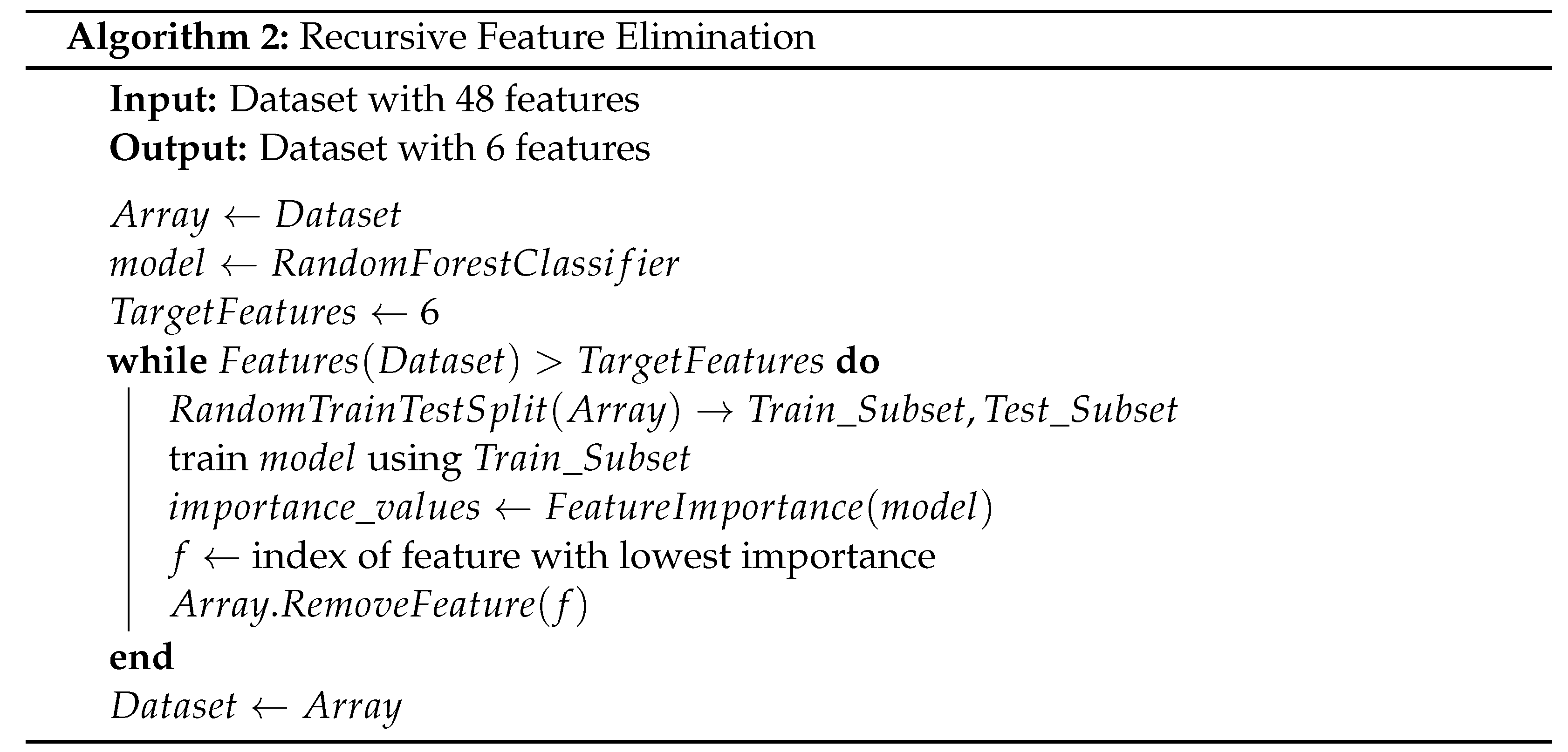
5. Proposed Feature Selection

6. Implementation and Results
6.1. Performance Metrics
- True Positive (TP );
- True Negative (TN);
- False Positive (FP);
- False Negative (FN).
- Accuracy
- Precision
- Recall
- Score
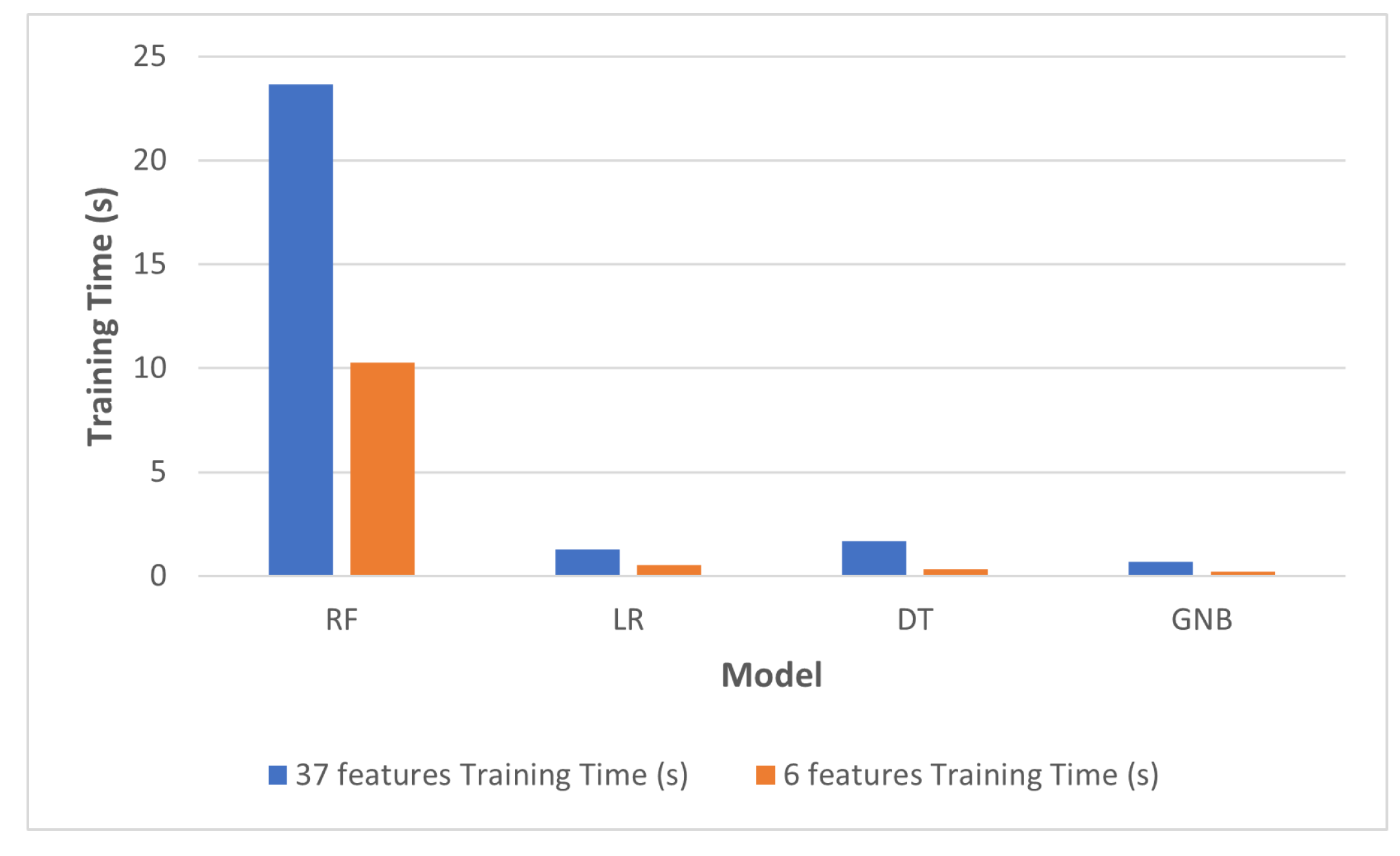
- Training TimeThe time spent in training the classifier (measured in seconds).
- Testing TimeThe time spent by the trained classifier to process one input instance and produce a prediction.
6.2. Testing Strategy
6.2.1. Initial Testing
6.2.2. Post Feature-Selection Testing
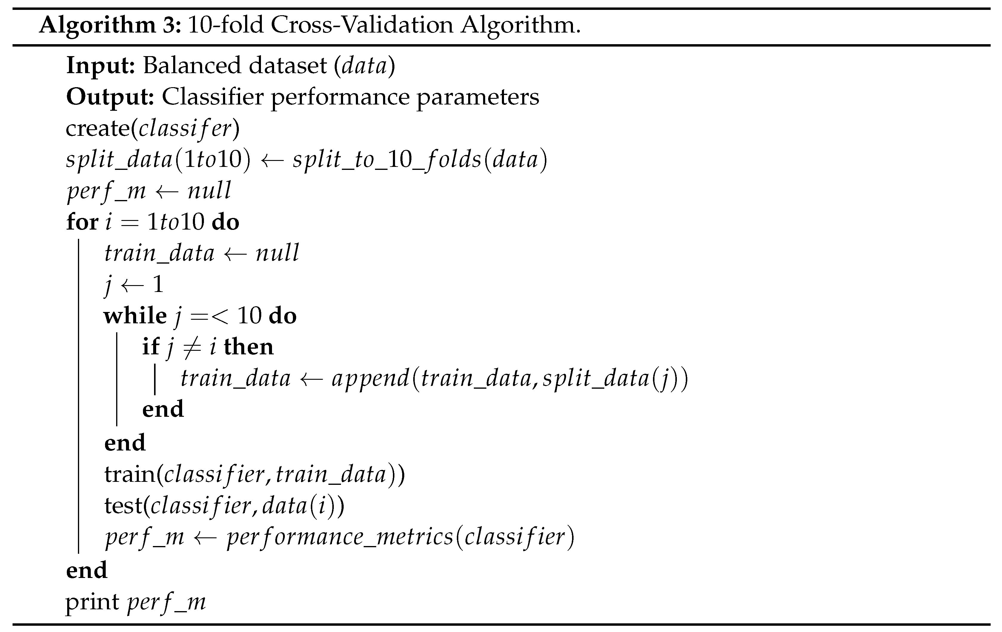
6.2.3. 10-Fold Cross-Validation

6.2.4. Testing with IoT-ID and Aposemat IoT-23 Datasets
6.2.5. Live Attack Testing
6.3. Testing Results
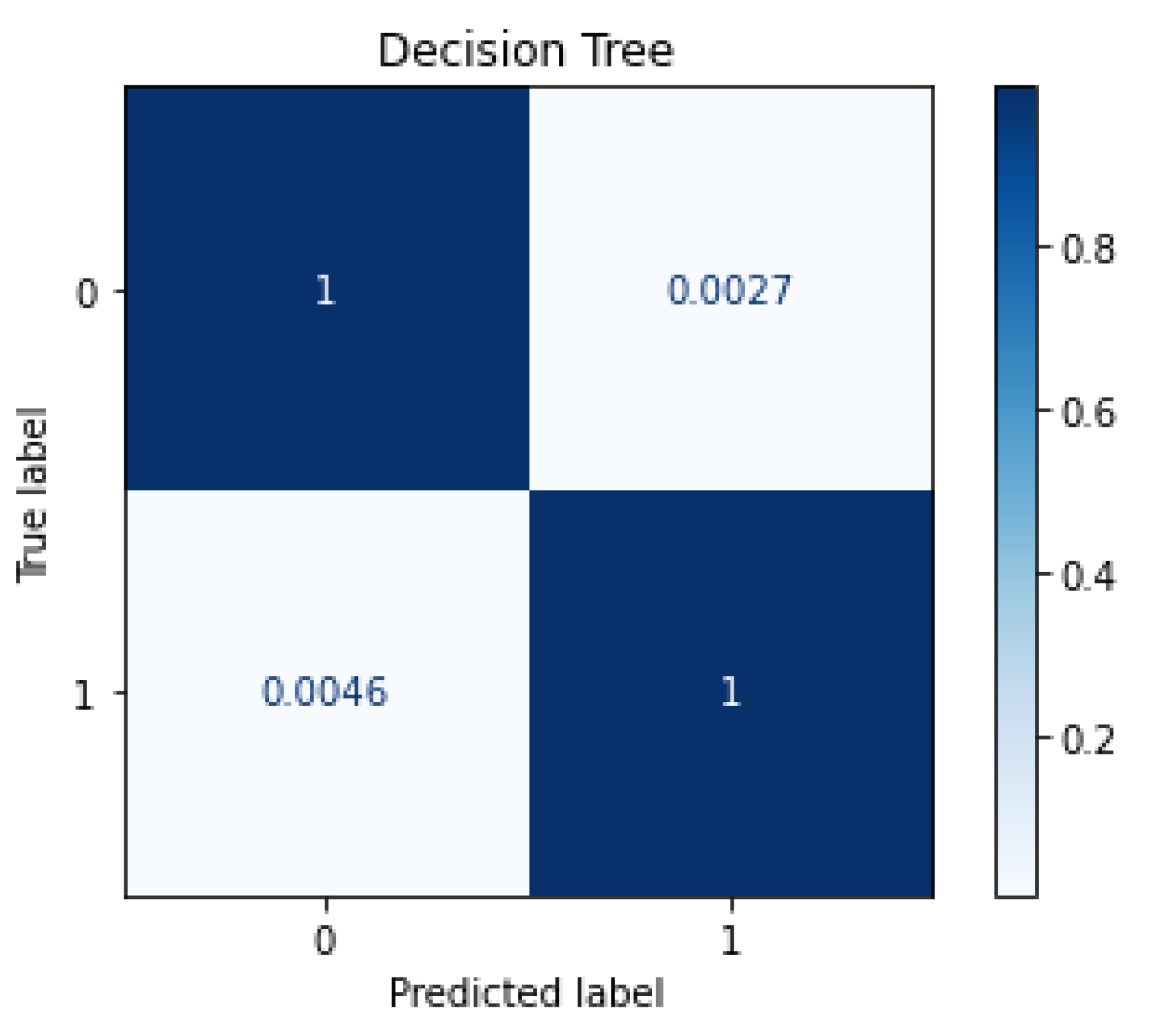
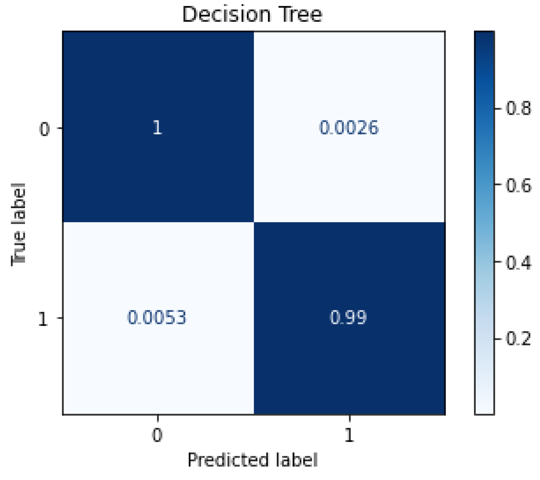
6.3.1. Testing before and after Feature Selection
6.3.2. 10-Fold Cross-Validation Results
6.3.3. Testing with IoT-ID and Aposemat IoT-23 Dataset
6.3.4. Live Attack Testing
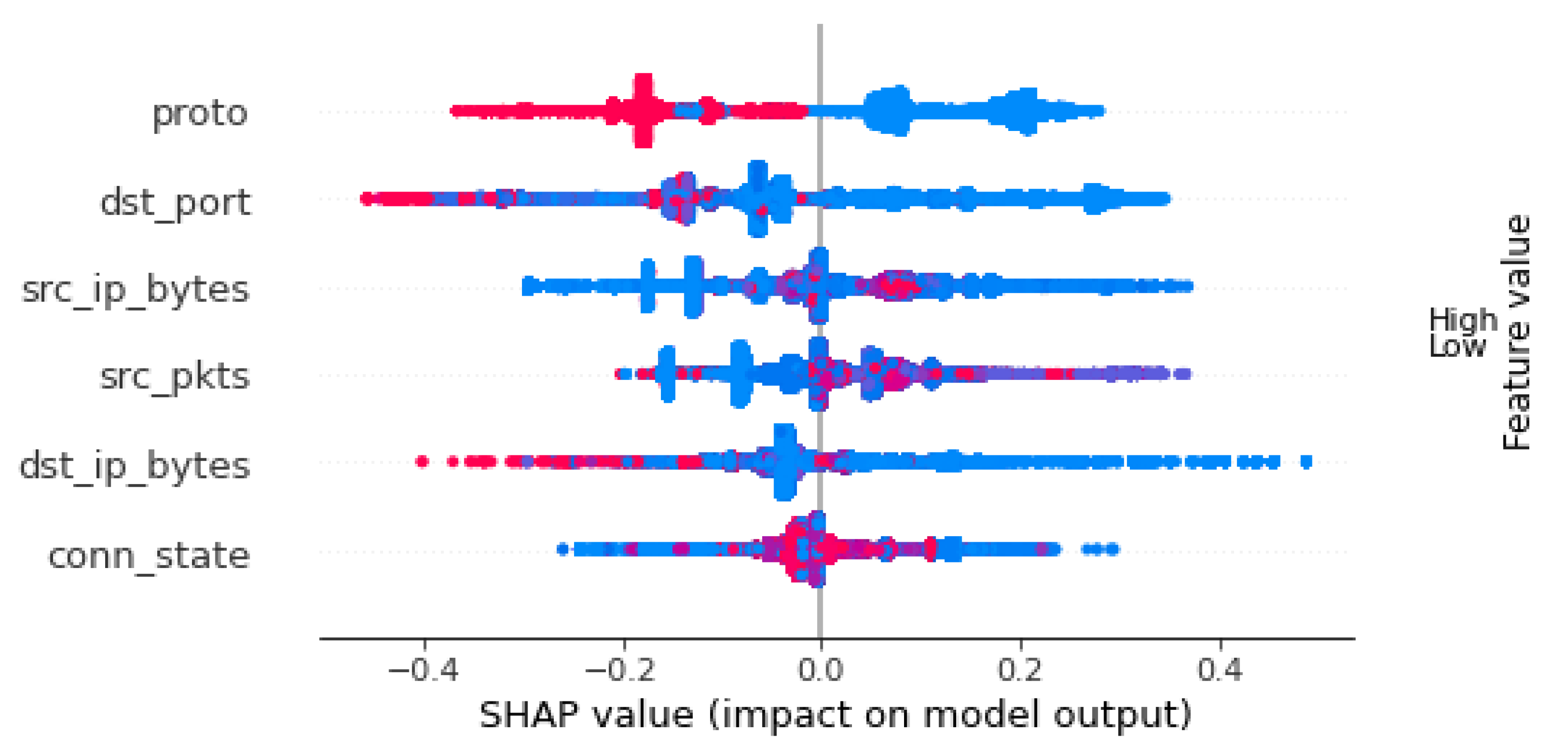
7. Model’s Explainability
8. Discussion
8.1. Implementation Considerations
- dst_port: The destination port number can be easily extracted from a single packet without the need of waiting for the network flow to end or timeout;
- conn_state: This feature can be identified by various connection states, such as S0 (connection without reply), S1 (connection established), and REJ (connection attempt rejected). This information is collected from the TCP headers throughout the network flow;
- src_pkts: Number of original packets which is sent from source device. This information is calculated based on the whole packet flow;
- proto: The transport layer protocol of the flow connection. This feature can also be extracted from the first packet in the connection without the need to wait for the flow to end;
- src_ip_bytes: Number of origin IP bytes which is the total length of IP header field of source systems. This can be calculated from the captured packet flow;
- dst_ip_bytes: Number of destination packets which is estimated from destination systems. This can be calculated from the captured packet flow.
8.2. Comparative Analysis
9. Conclusions and Future Work
- Measuring the performance of the trained model when deployed on border devices, such as firewall or proxy servers. This would help in having a better understanding of the practical requirements to make such systems operational;
- Measuring the performance of the trained model when deployed on IoT devices and measure their processing requirements and performance. This would help in understanding deployment requirements for the proposed system as a host-based IDS;
- Explore utilizing the reduced datasets in building deep neural networks. The utilization of deep neural networks can be explored in the context of network-based IDS to offset the processing load from the resource-constrained IoT devices to the border devices;
- Improving the performance of Algorithm 2 to reduce the time required for the feature selection process.
Author Contributions
Funding
Institutional Review Board Statement
Informed Consent Statement
Data Availability Statement
Conflicts of Interest
References
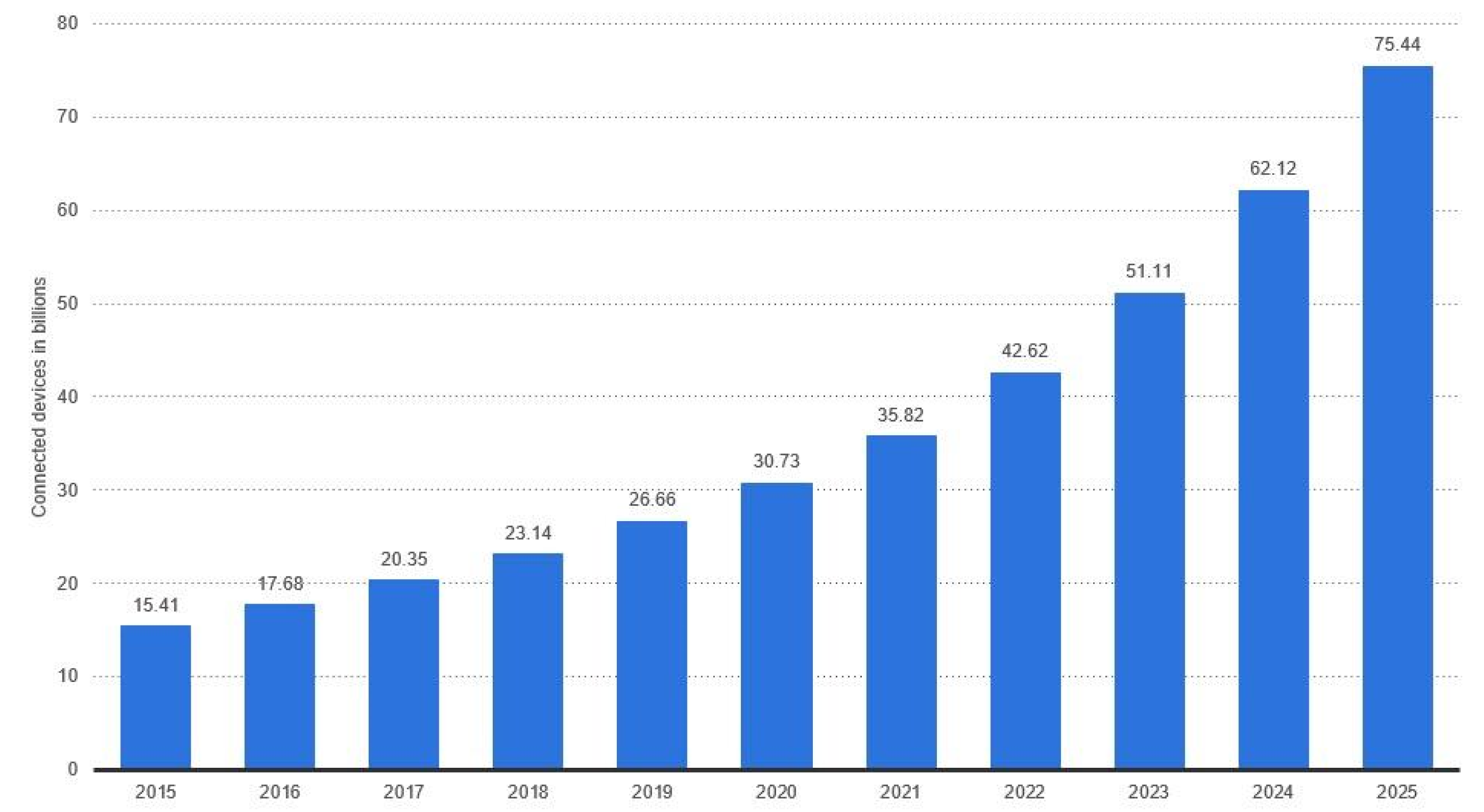
- Global IoT Connections Data Volume 2019 and 2025|Statista. 2022. Available online: https://www.statista.com/statistics/1017863/worldwide-iot-connected-devices-data-size/ (accessed on 23 February 2022).
- Internet of Threats: IoT Botnets Drive Surge in Network Attacks. 2021. Available online: https://securityintelligence.com/posts/internet-of-threats-iot-botnets-network-attacks/ (accessed on 21 January 2022).
- Seals, T. IoT Attacks Skyrocket, Doubling in 6 Months. Threatpost. 2021. Available online: https://threatpost.com/iot-attacks-doubling/169224 (accessed on 21 January 2022).
- Palmer, D. Critical IoT Security Camera Vulnerability Allows Attackers to Remotely Watch Live Video—And Gain Access to Networks. ZDNet 2021. Available online: https://www.zdnet.com/article/critical-iot-security-camera-vulnerability-allows-attackers-to-remotely-watch-live-video-and-gain-access-to-networks (accessed on 21 January 2022).
- Antonakakis, M.; April, T.; Bailey, M.; Bernhard, M.; Bursztein, E.; Cochran, J.; Durumeric, Z.; Halderman, J.A.; Invernizzi, L.; Kallitsis, M.; et al. Understanding the Mirai Botnet. In Proceedings of the 26th USENIX Security Symposium (USENIX Security 17), Vancouver, BC, Canada, 23 May 2017; USENIX Association: Berkeley, CA, USA, 2017; pp. 1093–1110. [Google Scholar]
- Liu, H.; Lang, B. Machine learning and deep learning methods for intrusion detection systems: A survey. Appl. Sci. 2019, 9, 4396. [Google Scholar] [CrossRef] [Green Version]
- Kilincer, I.F.; Ertam, F.; Sengur, A. Machine learning methods for cyber security intrusion detection: Datasets and comparative study. Comput. Netw. 2021, 188, 107840. [Google Scholar] [CrossRef]
- Asharf, J.; Moustafa, N.; Khurshid, H.; Debie, E.; Haider, W.; Wahab, A. A review of intrusion detection systems using machine and deep learning in internet of things: Challenges, solutions and future directions. Electronics 2020, 9, 1177. [Google Scholar] [CrossRef]
- Alsoufi, M.A.; Razak, S.; Siraj, M.M.; Nafea, I.; Ghaleb, F.A.; Saeed, F.; Nasser, M. Anomaly-based intrusion detection systems in iot using deep learning: A systematic literature review. Appl. Sci. 2021, 11, 8383. [Google Scholar] [CrossRef]
- Fatani, A.; Dahou, A.; Al-Qaness, M.A.; Lu, S.; Elaziz, M.A. Advanced feature extraction and selection approach using deep learning and Aquila optimizer for IoT intrusion detection system. Sensors 2021, 22, 140. [Google Scholar] [CrossRef] [PubMed]
- Desai, M.G.; Shi, Y.; Suo, K. IoT Bonet and Network Intrusion Detection using Dimensionality Reduction and Supervised Machine Learning. In Proceedings of the 2020 11th IEEE Annual Ubiquitous Computing, Electronics & Mobile Communication Conference (UEMCON), New York, NY, USA, 28–31 October 2020; pp. 0316–0322. [Google Scholar] [CrossRef]
- Kang, H.; Ahn, D.H.; Lee, G.M.; Yoo, J.D.; Park, K.H.; Kim, H.K. IoT Network Intrusion Dataset; IEEE: Piscataway, NJ, USA, 2019. [Google Scholar] [CrossRef]
- Moustafa, N. A new distributed architecture for evaluating AI-based security systems at the edge: Network TON_IoT datasets. Sustain. Cities Soc. 2021, 72, 102994. [Google Scholar] [CrossRef]
- Moustafa, N.; Ahmed, M.; Ahmed, S. Data Analytics-Enabled Intrusion Detection: Evaluations of ToN_IoT Linux Datasets. In Proceedings of the 2020 IEEE 19th International Conference on Trust, Security and Privacy in Computing and Communications (TrustCom), Guangzhou, China, 10–13 November 2020; pp. 727–735. [Google Scholar] [CrossRef]
- Nimbalkar, P.; Kshirsagar, D. Feature selection for intrusion detection system in Internet-of-Things (IoT). ICT Express 2021, 7, 177–181. [Google Scholar] [CrossRef]
- Sarhan, M.; Layeghy, S.; Portmann, M. Towards a standard feature set for network intrusion detection system datasets. Mob. Netw. Appl. 2022, 27, 357–370. [Google Scholar] [CrossRef]
- Alsaedi, A.; Moustafa, N.; Tari, Z.; Mahmood, A.; Anwar, A. TON_IoT telemetry dataset: A new generation dataset of IoT and IIoT for data-driven intrusion detection systems. IEEE Access 2020, 8, 165130–165150. [Google Scholar] [CrossRef]
- Stratosphere IPS. 2022. Available online: https://www.stratosphereips.org/datasets-iot23 (accessed on 23 June 2022).
- The Zeek Network Security Monitor. 2022. Available online: https://zeek.org (accessed on 29 January 2022).
- Parsebrologs. 2022. Available online: https://pypi.org/project/parsebrologs (accessed on 29 January 2022).
- Anowar, F.; Sadaoui, S.; Selim, B. Conceptual and empirical comparison of dimensionality reduction algorithms (pca, kpca, lda, mds, svd, lle, isomap, le, ica, t-sne). Comput. Sci. Rev. 2021, 40, 100378. [Google Scholar] [CrossRef]
- Raschka, S.; Liu, Y.; Mirjalili, V. Machine Learning with PyTorch and Scikit-Learn; Packt Publishing: Birmingham, UK, 2022. [Google Scholar]
- Kasongo, S.M.; Sun, Y. Performance Analysis of Intrusion Detection Systems Using a Feature Selection Method on the UNSW-NB15 Dataset. J. Big Data 2020, 7, 105. [Google Scholar] [CrossRef]
- Géron, A. Hands-on Machine Learning with Scikit-Learn, Keras, and TensorFlow: Concepts, Tools, and Techniques to Build Intelligent Systems; O’Reilly Media: Sebastopol, CA, USA, 2019. [Google Scholar]
- Nmap: The Network Mapper—Free Security Scanner. 2022. Available online: https://nmap.org (accessed on 15 July 2022).
- Molnar, C.; Casalicchio, G.; Bischl, B. Interpretable machine learning—A brief history, state-of-the-art and challenges. In Proceedings of the Joint European Conference on Machine Learning and Knowledge Discovery in Databases, Bilbao, Spain, 13–17 September 2020; Springer: Berlin/Heidelberg, Germany, 2020; pp. 417–431. [Google Scholar]
- Lundberg, S.M.; Lee, S.I. A Unified Approach to Interpreting Model Predictions. In Proceedings of the NIPS’17, Long Beach, CA, USA, 4–9 December 2017; Curran Associates Inc.: Red Hook, NY, USA, 2017; pp. 4768–4777. [Google Scholar]
- Khan, N.M.; Nalina Madhav, C.; Negi, A.; Thaseen, I.S. Analysis on Improving the Performance of Machine Learning Models Using Feature Selection Technique. In Intelligent Systems Design and Applications; Springer: Cham, Switzerland, 2019; pp. 69–77. [Google Scholar] [CrossRef]
- Kanimozhi, V.; Jacob, P. UNSW-NB15 Dataset Feature Selection and Network Intrusion Detection Using Deep Learning. Int. J. Recent Technol. Eng. 2019, 7, 443–446. [Google Scholar]
- Booij, T.M.; Chiscop, I.; Meeuwissen, E.; Moustafa, N.; den Hartog, F.T. ToN_IoT: The Role of Heterogeneity and the Need for Standardization of Features and Attack Types in IoT Network Intrusion Datasets. IEEE Internet Things J. 2021, 9, 484–496. [Google Scholar] [CrossRef]


| Traffic Category | Number of Packets |
|---|---|
| Benign | 300,000 |
| Backdoors | 20,000 |
| DoS | 20,000 |
| DDoS | 20,000 |
| Injection | 20,000 |
| Password | 20,000 |
| Ransomware | 20,000 |
| Scanning | 20,000 |
| Cross-Site Scripting | 20,000 |
| MITM | 1043 |
| 37 Features | 6 Features | |||||||
|---|---|---|---|---|---|---|---|---|
| Model | Accuracy | Score | FP | FN | Accuracy | Score | FP | FN |
| RF | 0.9992 | 0.9992 | 0.0007 | 0.0006 | 0.9966 | 0.9966 | 0.0025 | 0.0042 |
| LR | 0.6502 | 0.3946 | 0.0000 | 0.0001 | 0.6500 | 0.3940 | 0.0000 | 1.0000 |
| DT | 0.9989 | 0.9988 | 0.0009 | 0.0013 | 0.9962 | 0.9962 | 0.0027 | 0.0046 |
| GNB | 0.6501 | 0.3947 | 0.0003 | 1.0000 | 0.4246 | 0.3381 | 0.8700 | 0.0300 |
| Fold | Accuracy | Precision | Recall | Score |
|---|---|---|---|---|
| 1 | 0.997289 | 0.995432 | 0.996848 | 0.996139 |
| 2 | 0.997245 | 0.995867 | 0.996297 | 0.996082 |
| 3 | 0.996920 | 0.995136 | 0.996005 | 0.995570 |
| 4 | 0.996681 | 0.995882 | 0.994579 | 0.995230 |
| 5 | 0.997245 | 0.995903 | 0.996212 | 0.996057 |
| 6 | 0.996855 | 0.995465 | 0.995402 | 0.995434 |
| 7 | 0.996877 | 0.995075 | 0.995944 | 0.995509 |
| 8 | 0.997397 | 0.995525 | 0.997013 | 0.996268 |
| 9 | 0.996942 | 0.995100 | 0.996259 | 0.995679 |
| 10 | 0.997180 | 0.995502 | 0.996484 | 0.995993 |
| Mean | 0.997063 | 0.995489 | 0.996104 | 0.995796 |
| S-Dev | 0.000224 | 0.000304 | 0.000667 | 0.000336 |
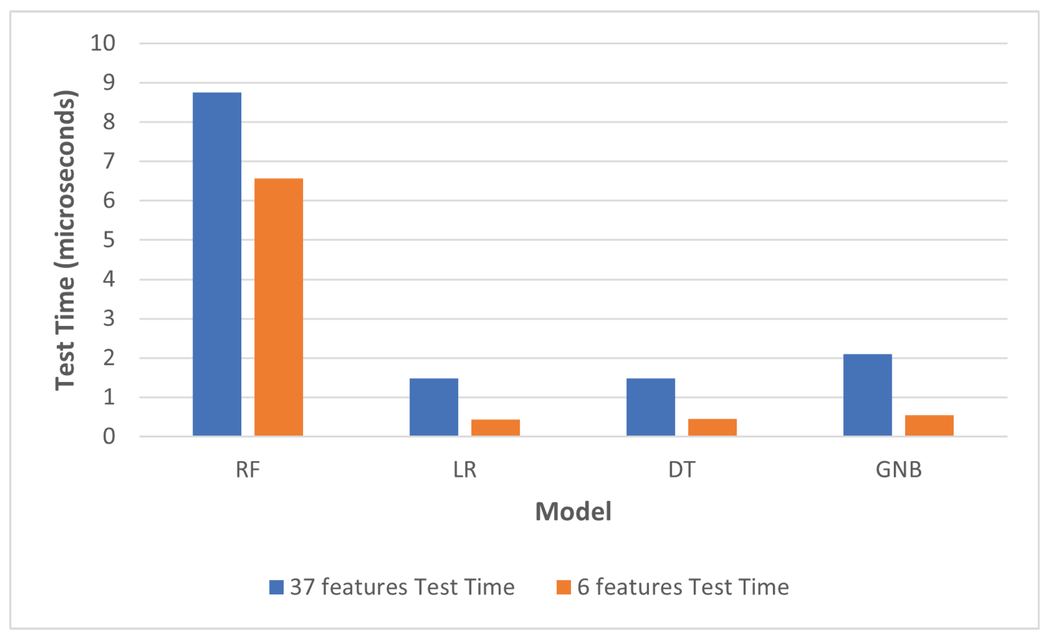
| 37 Features | 6 Features | |||
|---|---|---|---|---|
| Model | Train Time (s) | Test Time (s) | Train Time (s) | Test Time (s) |
| RF | 23.6616 | 8.7462 | 10.2907 | 6.5594 |
| LR | 1.3017 | 1.4834 | 0.5439 | 0.4346 |
| DT | 1.6723 | 1.4851 | 0.3339 | 0.4549 |
| GNB | 0.6859 | 2.0967 | 0.2129 | 0.5418 |
| Paper | Dataset | Features | Classifier | Accuracy (%) | Training T (s) | Testing T (s) |
|---|---|---|---|---|---|---|
| [15] | IoT-BoT | 16 | JRip | 99.992 | 80.94 | - |
| [17] | TON_IoT | 44 | CART | 88 | 6.308 | 0.022 |
| RF | 85 | 10.884 | 0.164 | |||
| KNN | 84 | 58.018 | 109.361 | |||
| LSTM | 81 | 1596 | 9.023 | |||
| [30] | TON_IoT | 13 | ANN | 84.39 | - | - |
| and | GBM | 99.897 | - | - | ||
| Aposemat | RF | 99.931 | - | - | ||
| IoT-23 | MLP | 99.022 | - | - | ||
| [16] | TON_IoT | 43 | Extra Tree | 97.86% | - | 8.93 s |
| Our work | TON_IoT | 6 | DT | 99.62 | 0.3339 | 0.4549 s |
| IoT-ID | 6 | DT | 99.63 | 0.3528 | 0.4663 s | |
| Aposemat-IoT-23 | 6 | DT | 99.61 | 0.2973 | 0.4682 s |
Publisher’s Note: MDPI stays neutral with regard to jurisdictional claims in published maps and institutional affiliations. |
© 2022 by the authors. Licensee MDPI, Basel, Switzerland. This article is an open access article distributed under the terms and conditions of the Creative Commons Attribution (CC BY) license (https://creativecommons.org/licenses/by/4.0/).
Share and Cite
Alani, M.M.; Miri, A. Towards an Explainable Universal Feature Set for IoT Intrusion Detection. Sensors 2022, 22, 5690. https://doi.org/10.3390/s22155690
Alani MM, Miri A. Towards an Explainable Universal Feature Set for IoT Intrusion Detection. Sensors. 2022; 22(15):5690. https://doi.org/10.3390/s22155690
Chicago/Turabian StyleAlani, Mohammed M., and Ali Miri. 2022. "Towards an Explainable Universal Feature Set for IoT Intrusion Detection" Sensors 22, no. 15: 5690. https://doi.org/10.3390/s22155690