
Comparison of Deep Learning Algorithms in Predicting Expert Assessments of Pain Scores during Surgical Operations Using Analgesia Nociception Index

 ,
,  and
and
Abstract
:1. Introduction
2. Materials and Method
2.1. Patients and ECG Signal
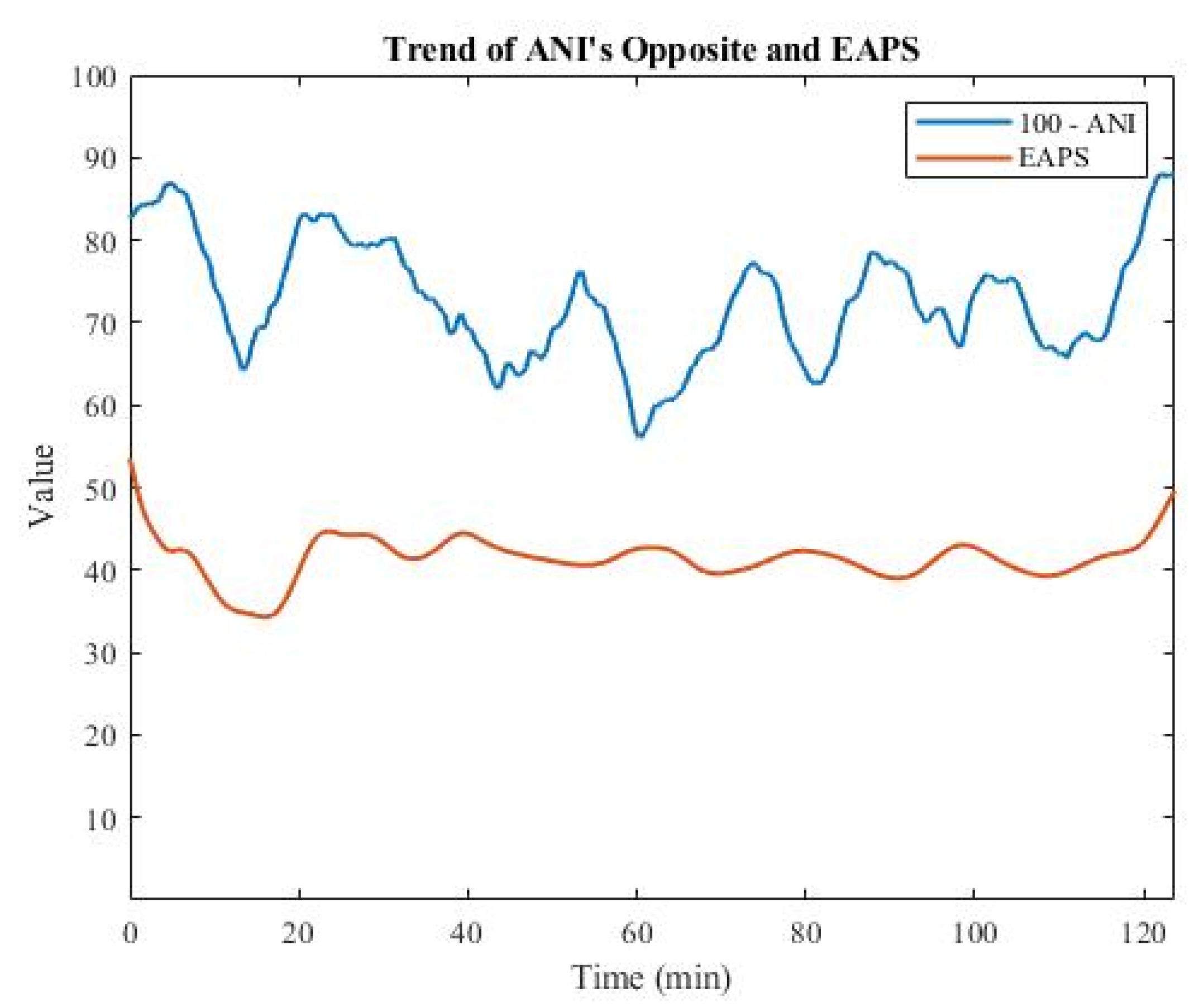
2.2. Expert Assessment of Pain Score (EAPS)
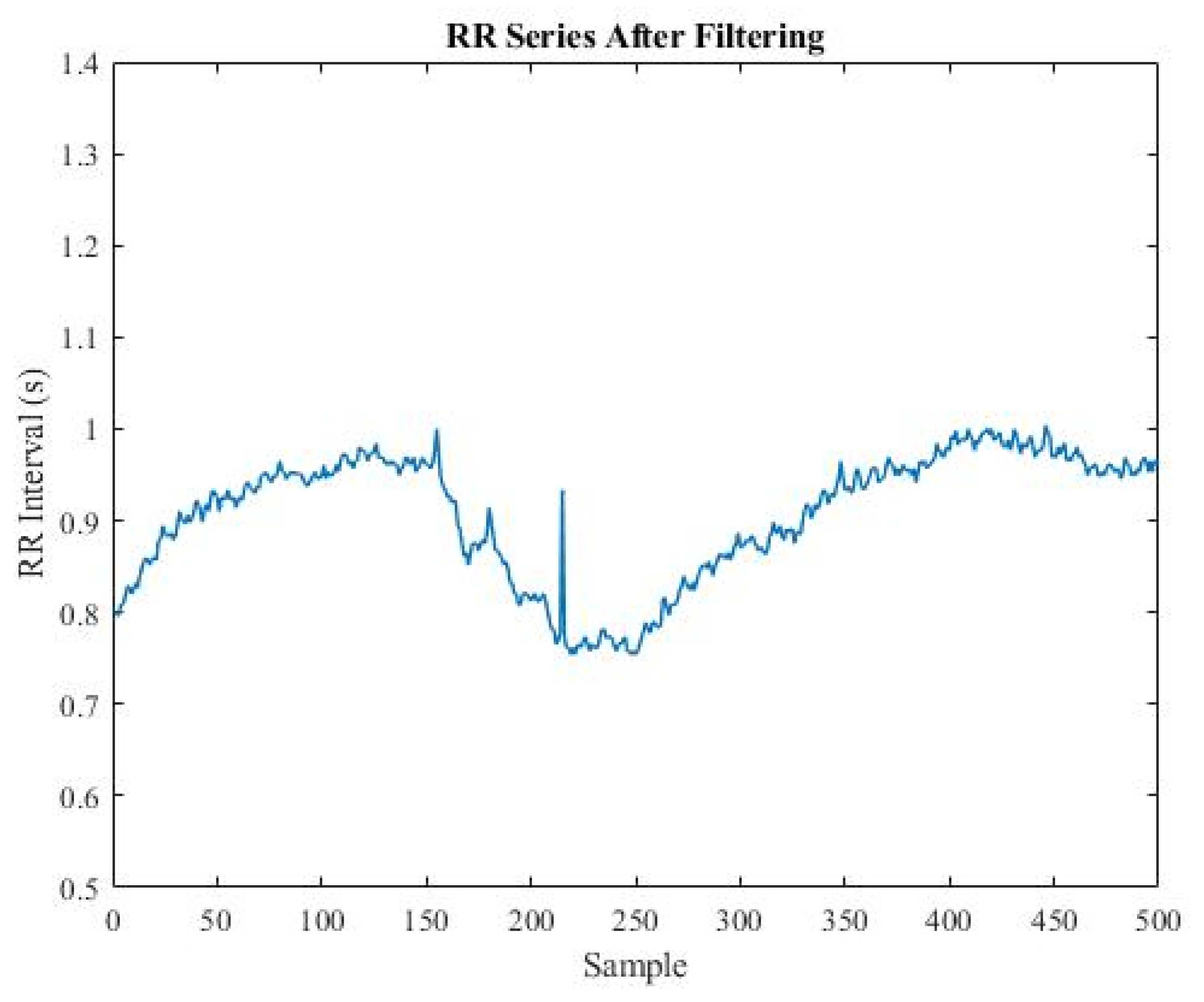
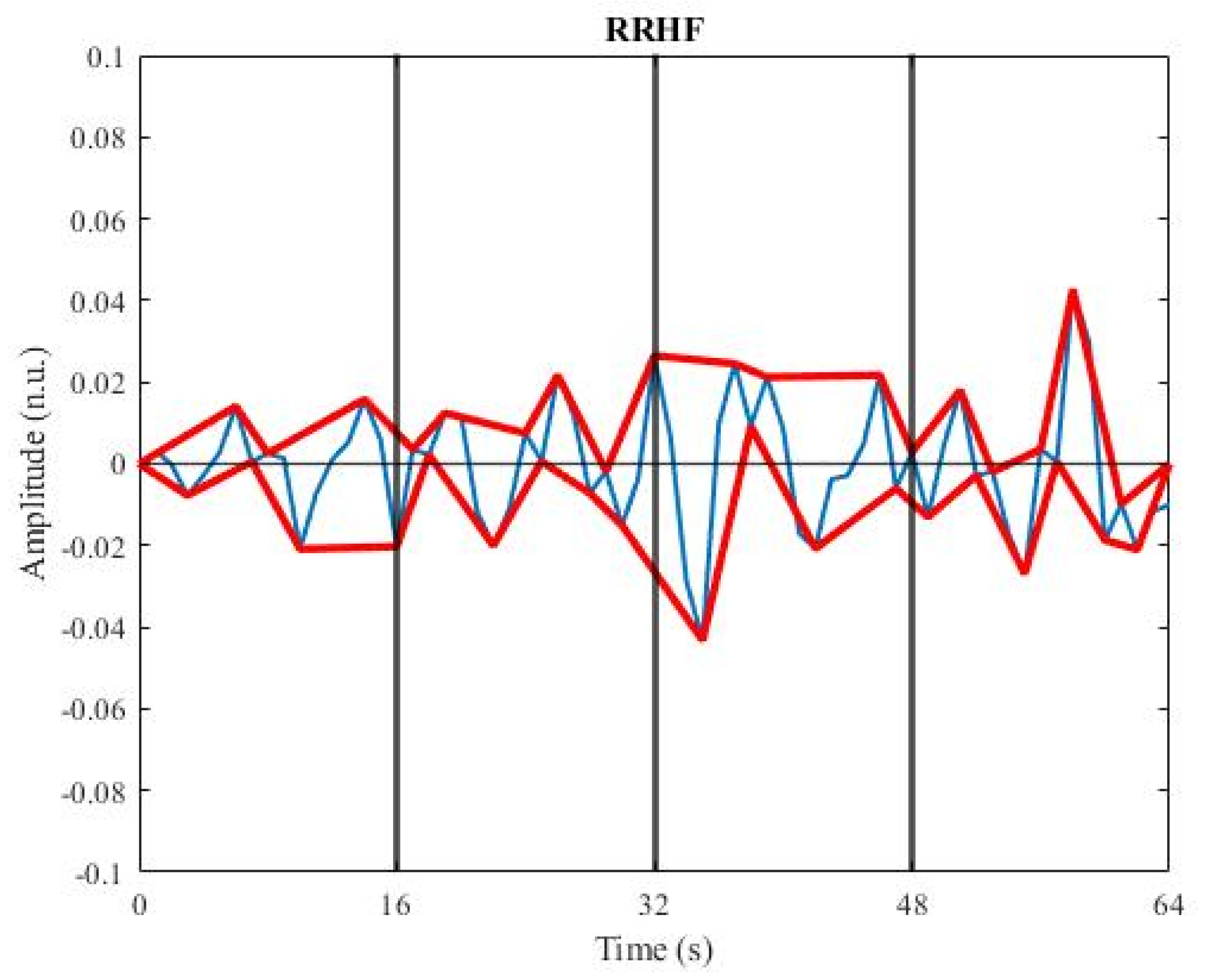
2.3. Calculation of ANI
- 1.
- and
- 2.
- or
- 3.
- : the -th sample of the RR series
- : the mean of the previous five samples
- : the standard deviation of the previous five samples
- 1.
- 2.
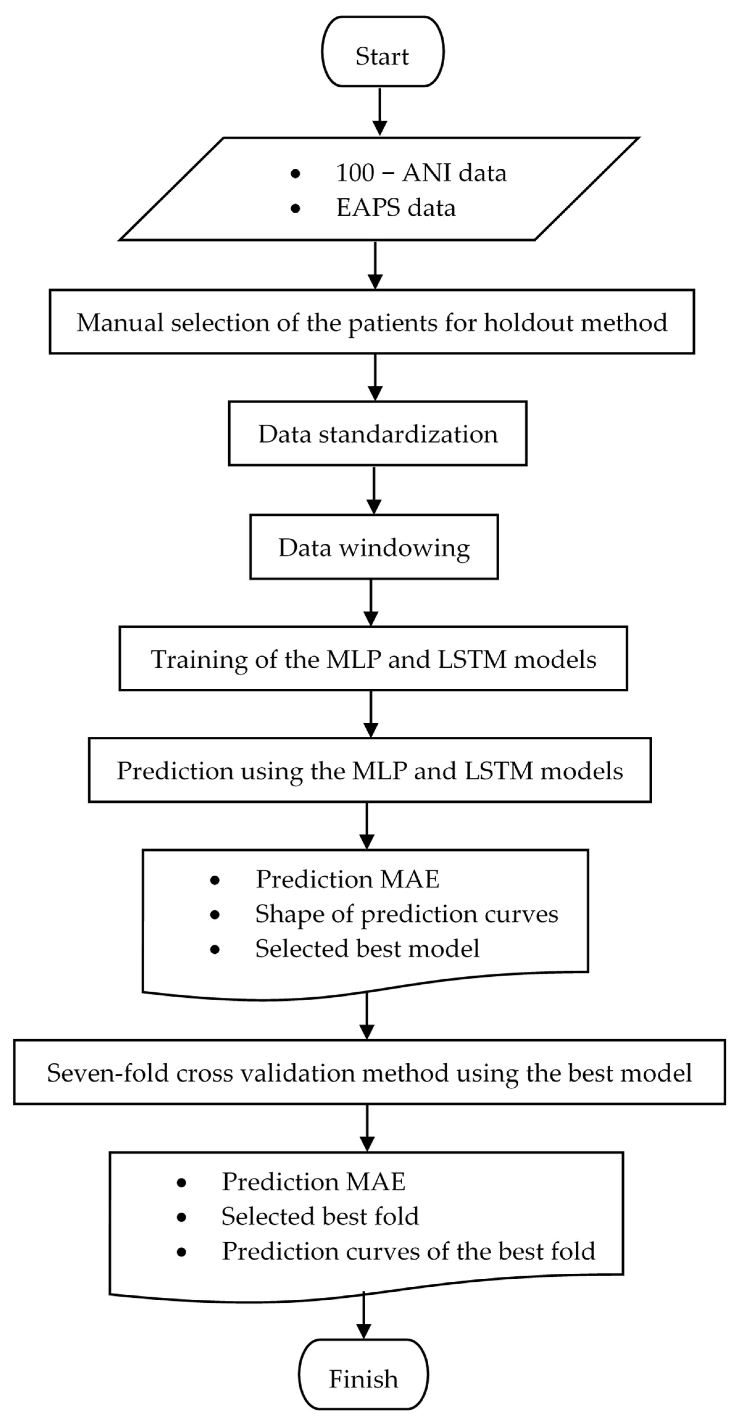
2.4. Deep Learning Models
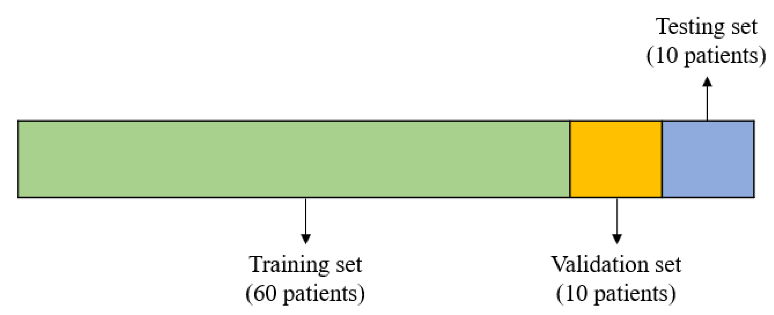
2.4.1. Holdout
2.4.2. Data Standardization
- : The standardized data
- : The data to be standardized
- : The mean of the training set
- : The standard deviation of the training set
2.4.3. Data Windowing
2.4.4. MLP Model
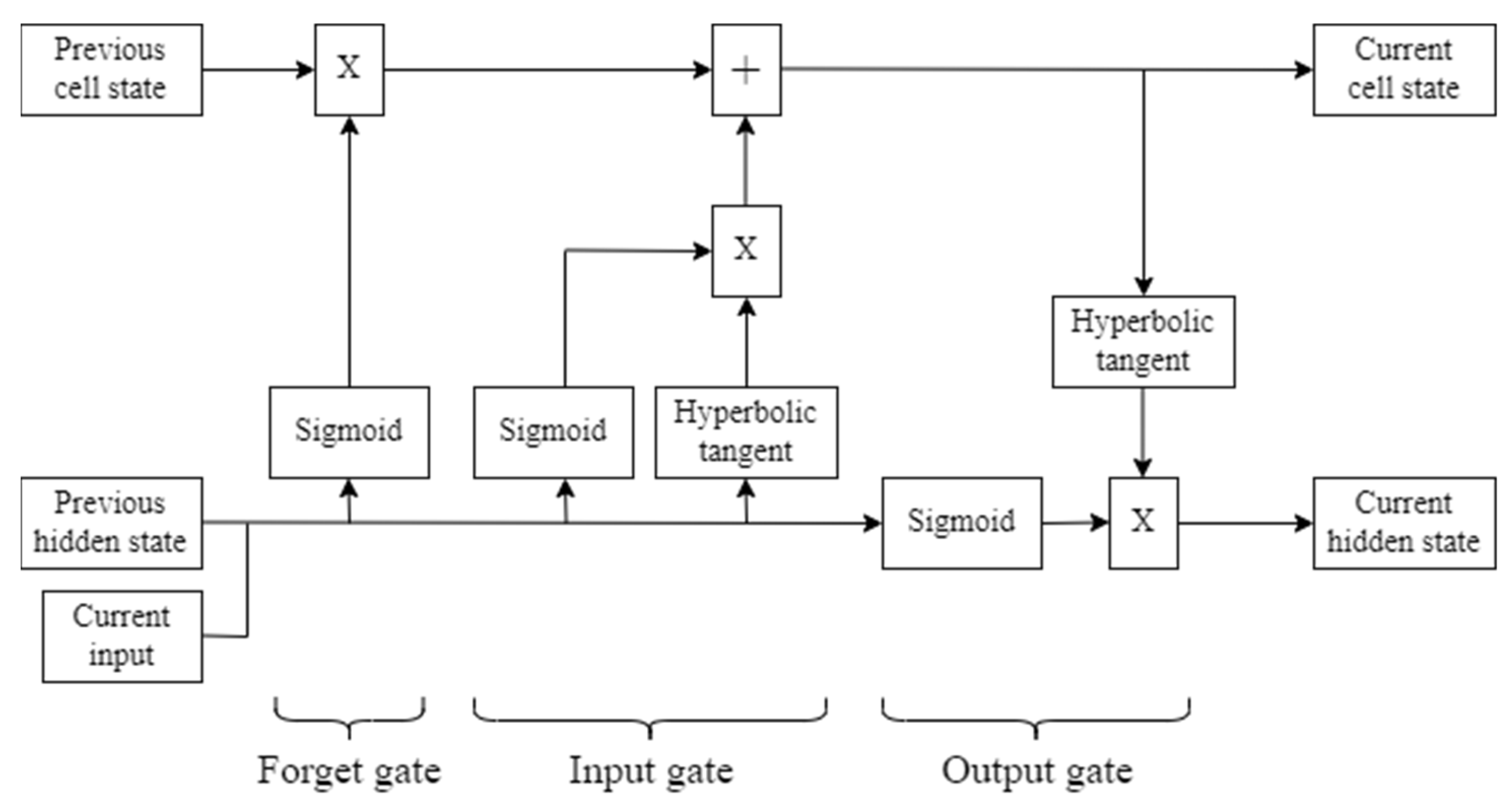
2.4.5. LSTM Model
2.4.6. Model Selection
2.4.7. Seven-Fold Cross Validation
3. Results
3.1. Analysis of EAPS Data
3.2. MLP and LSTM Models in the Holdout Method
3.3. Seven-Fold Cross Validation with MLP
4. Discussion
5. Conclusions
Supplementary Materials
Author Contributions
Funding
Institutional Review Board Statement
Informed Consent Statement
Data Availability Statement
Acknowledgments
Conflicts of Interest
References
- Jeanne, M.; Clément, C.; De Jonckheere, J.; Logier, R.; Tavernier, B. Variations of the analgesia nociception index during general anaesthesia for laparoscopic abdominal surgery. Int. J. Clin. Monit. Comput. 2012, 26, 289–294. [Google Scholar] [CrossRef] [PubMed]
- Chen, J.; Abbod, M.; Shieh, J.-S. Pain and stress detection using wearable sensors and devices—A review. Sensors 2021, 21, 1030. [Google Scholar] [CrossRef] [PubMed]
- Gruenewald, M.; Ilies, C.; Herz, J.; Schoenherr, T.; Fudickar, A.; Höcker, J.; Bein, B. Influence of nociceptive stimulation on analgesia nociception index (ANI) during propofol–remifentanil anaesthesia. Br. J. Anaesth. 2013, 110, 1024–1030. [Google Scholar] [CrossRef] [PubMed] [Green Version]
- Logier, R.; Jeanne, M.; De Jonckheere, J.; Dassonneville, A.; Delecroix, M.; Tavernier, B. PhysioDoloris: A Monitoring Device for Analgesia/Nociception Balance Evaluation Using Heart Rate Variability Analysis. In Proceedings of the 2010 Annual International Conference of the IEEE Engineering in Medicine and Biology, Buenos Aires, Argentina, 31 August–4 September 2010; pp. 1194–1197. [Google Scholar] [CrossRef]
- Turan, G.; Ar, A.Y.; Kuplay, Y.Y.; Demiroluk, O.; Gazi, M.; Akgun, N.; Celikoglu, E. Analgesia nociception index for perioperative analgesia monitoring in spinal surgery. Rev. Bras. De Anestesiol. 2017, 67, 370–375. [Google Scholar] [CrossRef] [PubMed]
- Abdullayev, R.; Uludag, O.; Celik, B. Analgesia Nociception Index: Assessment of acute postoperative pain. Rev. Bras. De Anestesiol. 2019, 69, 396–402. [Google Scholar] [CrossRef]
- Abdullayev, R.; Yildirim, E.; Celik, B.; Sarica, L.T. Analgesia nociception index: Heart rate variability analysis of emotional status. Cureus 2019, 11, e4365. [Google Scholar] [CrossRef] [PubMed] [Green Version]
- Shapiro, S.C. Artificial Intelligence (AI) in Encyclopedia of Computer Science; John Wiley and Sons Ltd.: Chichester, UK, 2003; pp. 89–93. [Google Scholar]
- Ramesh, A.N.; Kambhampati, C.; Monson, J.; Drew, P. Artificial Intelligence in Medicine. Ann. R. Coll. Surg. Engl. 2004, 86, 334–338. [Google Scholar] [CrossRef] [PubMed] [Green Version]
- de Silva, I.N.; Spatti, D.H.; Flauzino, R.A.; Liboni, L.H.B.; dos Reis Alves, S.F. Artificial Neural Networks: A Practical Course; Springer: Cham, Switzerland, 2017. [Google Scholar]
- Hochreiter, S.; Schmidhuber, J. Long short-term memory. Neural Comput. 1997, 9, 1735–1780. [Google Scholar] [CrossRef] [PubMed]
- Brownlee, J. Long Short-Term Memory Networks with Python: Develop Sequence Prediction Models with Deep Learning; Machine Learning Mastery: San Juan, Puerto Rico, 2017. [Google Scholar]
- Zebin, T.; Sperrin, M.; Peek, N.; Casson, A.J. Human Activity Recognition from Inertial Sensor Time-Series Using Batch Normalized Deep LSTM Recurrent Networks. In Proceedings of the Annual International Conference of the IEEE Engineering in Medicine and Biology Society, Honolulu, HI, USA, 18–21 July 2018. [Google Scholar]
- Hans, P.; Verscheure, S.; Uutela, K.; Hans, G.; Bonhomme, V. Effect of a fluid challenge on the Surgical Pleth Index during stable propofol-remifentanil anaesthesia. Acta Anaesthesiol. Scand. 2012, 56, 787–796. [Google Scholar] [CrossRef] [PubMed]
- Hu, S.B.; Wong, D.J.L.; Correa, A.; Li, N.; Deng, J.C. Prediction of clinical deterioration in hospitalized adult patients with hematologic malignancies using a neural network model. PLoS ONE 2016, 11, e0161401. [Google Scholar] [CrossRef] [PubMed] [Green Version]
- Sadrawi, M.; Fan, S.-Z.; Abbod, M.F.; Jen, K.-K.; Shieh, J.-S. Computational Depth of Anesthesia via Multiple Vital Signs Based on Artificial Neural Networks. BioMed. Res. Int. 2015, 2015, 536863. [Google Scholar] [CrossRef] [Green Version]
- Sharifi, A.; Alizadeh, K. A novel classification method based on multilayer perceptron-artificial neural network technique for diagnosis of chronic kidney disease. Ann. Mil. Health Sci. Res. 2020, 18, e101585. [Google Scholar] [CrossRef]
- Kim, J.; Chae, M.; Chang, H.-J.; Kim, Y.-A.; Park, E. Predicting Cardiac Arrest and Respiratory Failure Using Feasible Artificial Intelligence with Simple Trajectories of Patient Data. J. Clin. Med. 2019, 8, 1336. [Google Scholar] [CrossRef] [PubMed] [Green Version]
- Sideris, C.; Kalantarian, H.; Nemati, E.; Sarrafzadeh, M. Building Continuous Arterial Blood Pressure Prediction Models Using Recurrent Networks. In Proceedings of the 2016 IEEE International Conference on Smart Computing (SMARTCOMP), St. Louis, MO, USA, 18–20 May 2016. [Google Scholar]
- Jiang, G.J.A.; Fan, S.-Z.; Abbod, M.F.; Huang, H.-H.; Lan, J.-Y.; Tsai, F.-F.; Chang, H.-C.; Yang, Y.-W.; Chuang, F.-L.; Chiu, Y.-F.; et al. Sample entropy analysis of EEG signals via artificial neural networks to model patients’ consciousness level based on anesthesiologists experience. BioMed. Res. Int. 2015, 2015, 343478. [Google Scholar] [CrossRef] [PubMed]
- Logier, R.; Jonckheere, J.D.; Dassonneville, A. An Efficient Algorithm for R-R Intervals Series Filtering. In Proceedings of the 26th Annual International Conference of the IEEE EMBS, San Francisco, CA, USA, 1–5 September 2004. [Google Scholar]
- Jeanne, M.; Logier, R.; Jonckheere, J.D.; Tavernier, B. Validation of A Graphic Measurement of Heart Rate Variability to Assess Analgesia/Nociception Balance during General Anesthesia. In Proceedings of the 31st Annual International Conference of the IEEE EMBS, Minnesota, MN, USA, 2–6 September 2009. [Google Scholar]
- Jonckheere, J.D.; Rommel, D.; Nandrino, J.L.; Jeanne, M.; Logier, R. Heart Rate Variability Analysis as an Index of Emotion Regulation Processes: Interest of the Analgesia Nociception Index (ANI). In Proceedings of the 34th Annual International Conference of the IEEE EMBS, San Diego, CA, USA, 10 November 2012. [Google Scholar]


| No. | Set | Number of Patients | Number of Windows |
|---|---|---|---|
| 1 | Training | 60 | 47,554 |
| 2 | Validation | 10 | 9031 |
| 3 | Testing | 10 | 9374 |
| Variable | MLP | LSTM |
|---|---|---|
| Training Loss | 2.847 | 2.859 |
| Validation Loss | 2.933 | 3.194 |
| Testing Patient | MAE of MLP | MAE of LSTM |
|---|---|---|
| 1 | 2.716 | 3.238 |
| 2 | 2.622 | 3.493 |
| 3 | 3.422 | 2.271 |
| 4 | 2.118 | 1.886 |
| 5 | 2.127 | 2.768 |
| 6 | 1.875 | 1.948 |
| 7 | 1.933 | 2.242 |
| 8 | 2.735 | 3.076 |
| 9 | 2.214 | 2.671 |
| 10 | 3.138 | 2.731 |
| Overall (mean ± SD) | 2.490 ± 0.522 | 2.633 ± 0.542 |
| Fold | Training Loss | Validation Loss | Overall Prediction MAE (Mean ± SD) |
|---|---|---|---|
| 1 | 2.832 | 2.863 | 2.460 ± 0.634 |
| 2 | 2.793 | 3.195 | 3.075 ± 0.879 |
| 3 | 2.795 | 3.738 | 3.041 ± 0.673 |
| 4 | 2.869 | 2.640 | 2.542 ± 0.711 |
| 5 | 2.754 | 3.114 | 3.031 ± 0.948 |
| 6 | 2.804 | 3.799 | 3.209 ± 0.820 |
| 7 | 2.788 | 2.830 | 2.581 ± 0.711 |
| Fold | MAE |
|---|---|
| 1 | 2.460 |
| 2 | 3.075 |
| 3 | 3.041 |
| 4 | 2.542 |
| 5 | 3.031 |
| 6 | 3.209 |
| 7 | 2.581 |
| Overall (mean ± SD) | 2.848 ± 0.308 |
Publisher’s Note: MDPI stays neutral with regard to jurisdictional claims in published maps and institutional affiliations. |
© 2022 by the authors. Licensee MDPI, Basel, Switzerland. This article is an open access article distributed under the terms and conditions of the Creative Commons Attribution (CC BY) license (https://creativecommons.org/licenses/by/4.0/).
Share and Cite
Jean, W.-H.; Sutikno, P.; Fan, S.-Z.; Abbod, M.F.; Shieh, J.-S. Comparison of Deep Learning Algorithms in Predicting Expert Assessments of Pain Scores during Surgical Operations Using Analgesia Nociception Index. Sensors 2022, 22, 5496. https://doi.org/10.3390/s22155496
Jean W-H, Sutikno P, Fan S-Z, Abbod MF, Shieh J-S. Comparison of Deep Learning Algorithms in Predicting Expert Assessments of Pain Scores during Surgical Operations Using Analgesia Nociception Index. Sensors. 2022; 22(15):5496. https://doi.org/10.3390/s22155496
Chicago/Turabian StyleJean, Wei-Horng, Peter Sutikno, Shou-Zen Fan, Maysam F. Abbod, and Jiann-Shing Shieh. 2022. "Comparison of Deep Learning Algorithms in Predicting Expert Assessments of Pain Scores during Surgical Operations Using Analgesia Nociception Index" Sensors 22, no. 15: 5496. https://doi.org/10.3390/s22155496