
Intelligent Scheduling Methodology for UAV Swarm Remote Sensing in Distributed Photovoltaic Array Maintenance

Abstract
:1. Introduction
2. UAV Swarm Scheduling Model Based on Large-Scale Global Optimization
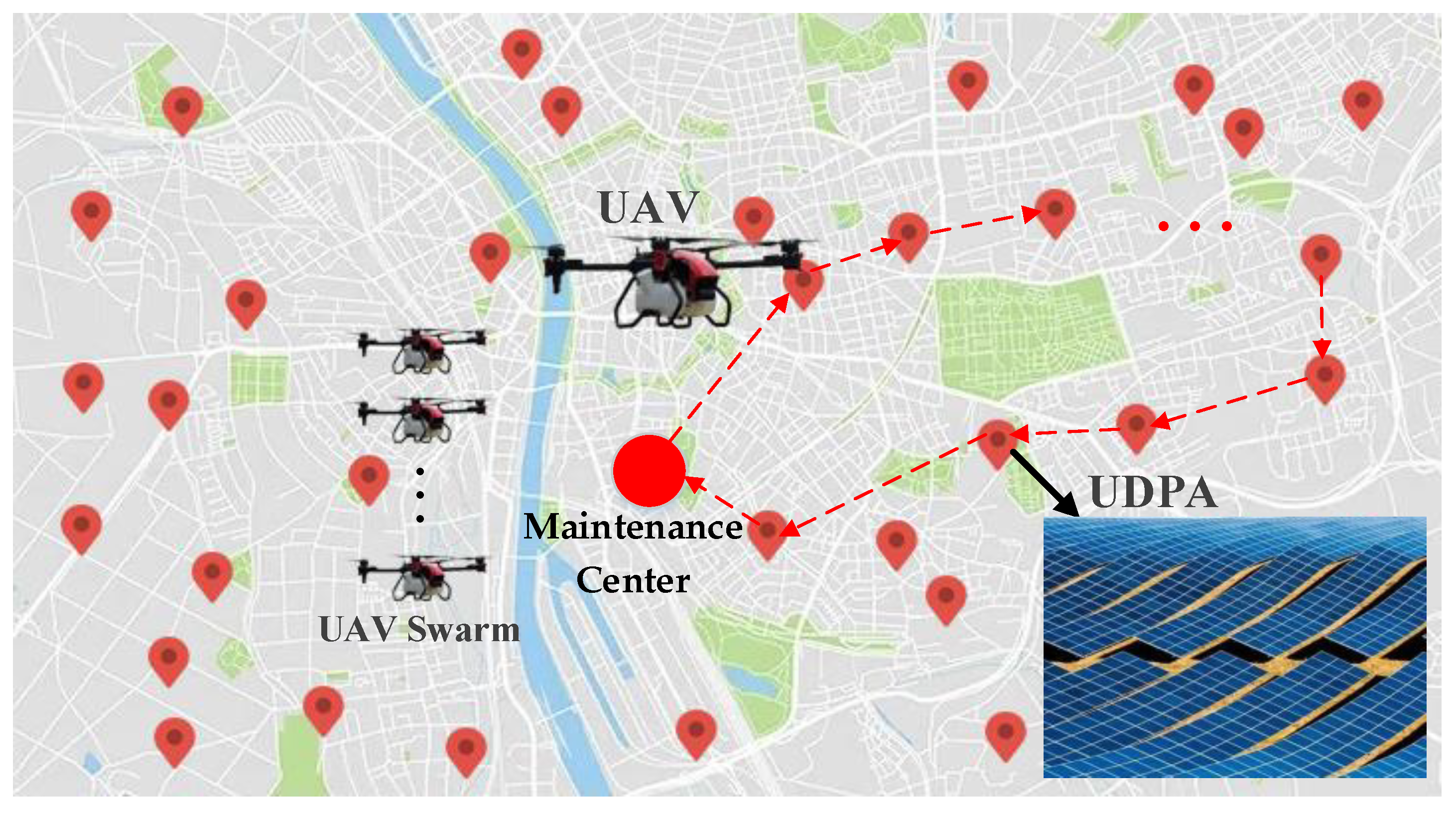
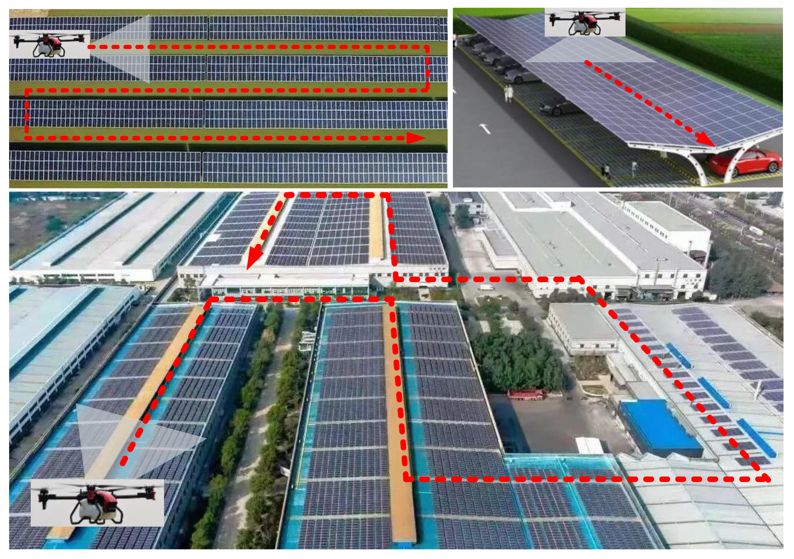
2.1. UAV Swarm Remote Sensing in UDPA Maintenance
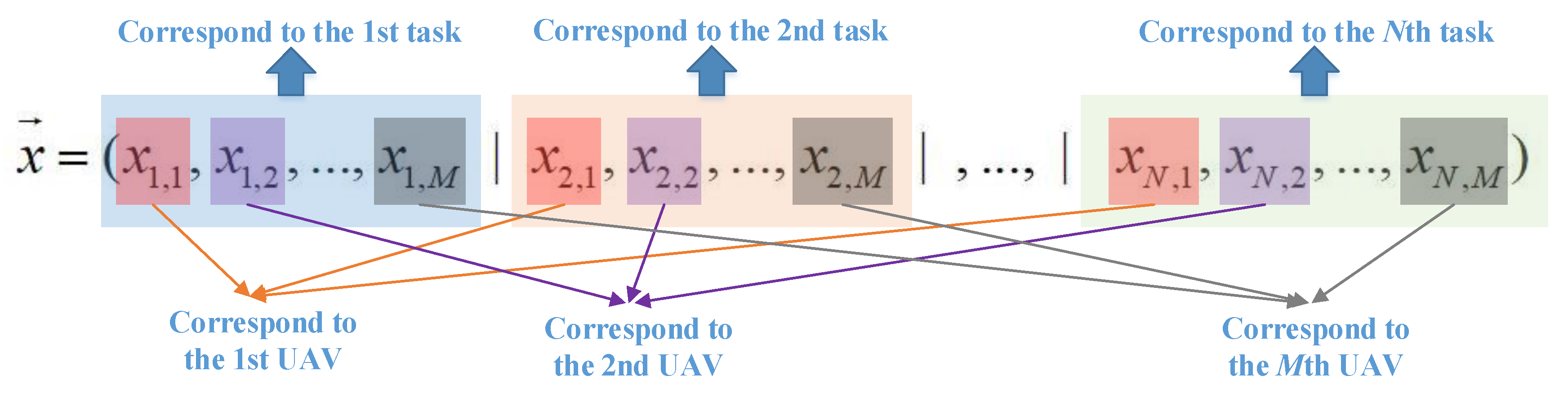
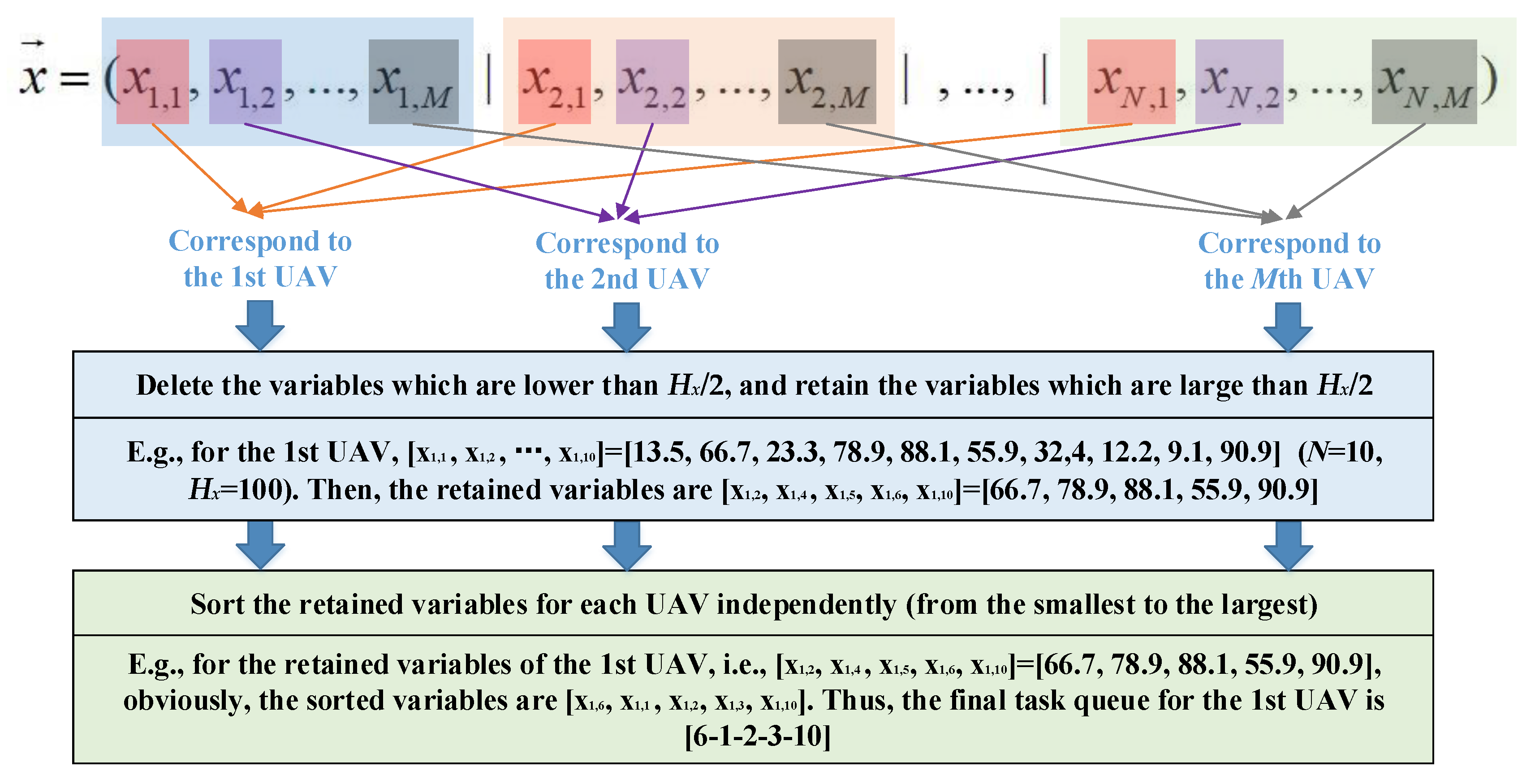
2.2. Encoding and Decoding Schemes
2.3. Constraints and Penalty Function
- (1)
- UAV duration constraint
- (2)
- Task-allocation constraint
- (3)
- UAV-utilization constraint
- (4)
- Penalty function
3. A Novel CCPSO-mg-cvcm Optimization Algorithm
3.1. Particle Swarm Optimization
3.2. Cooperatively Coevolving
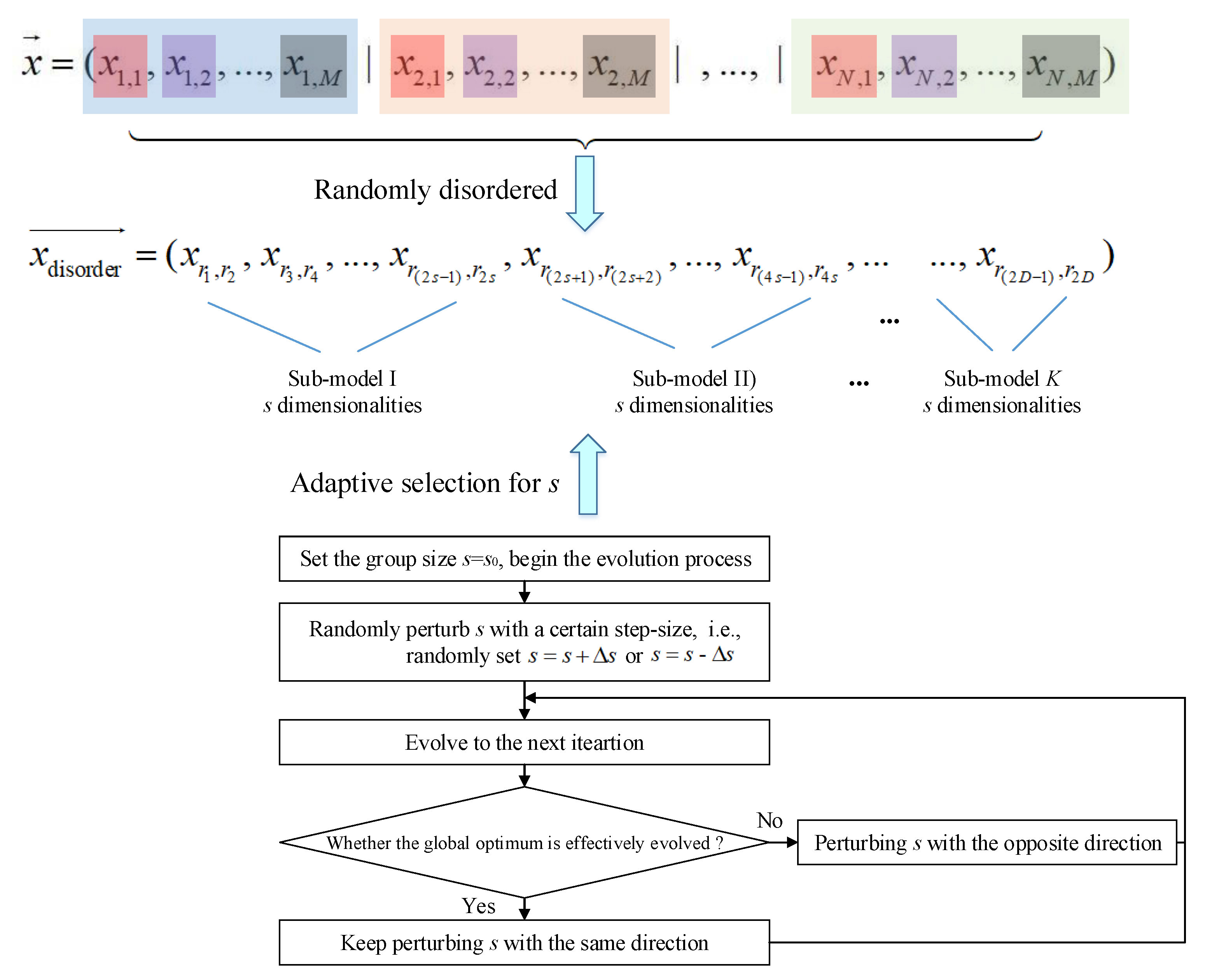
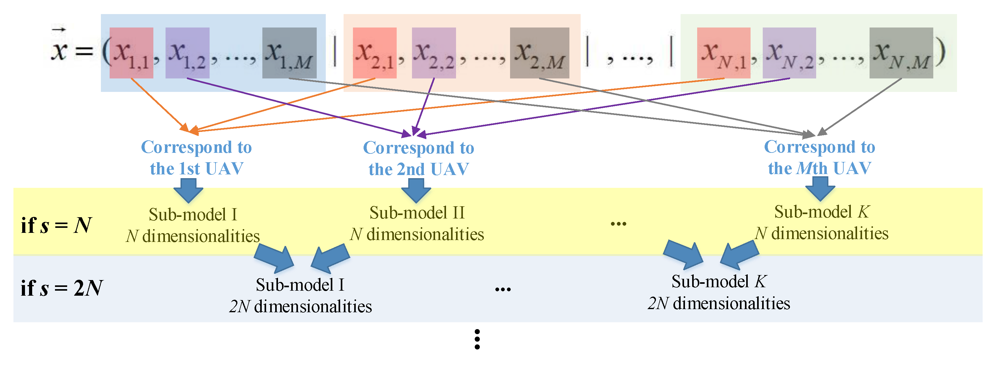
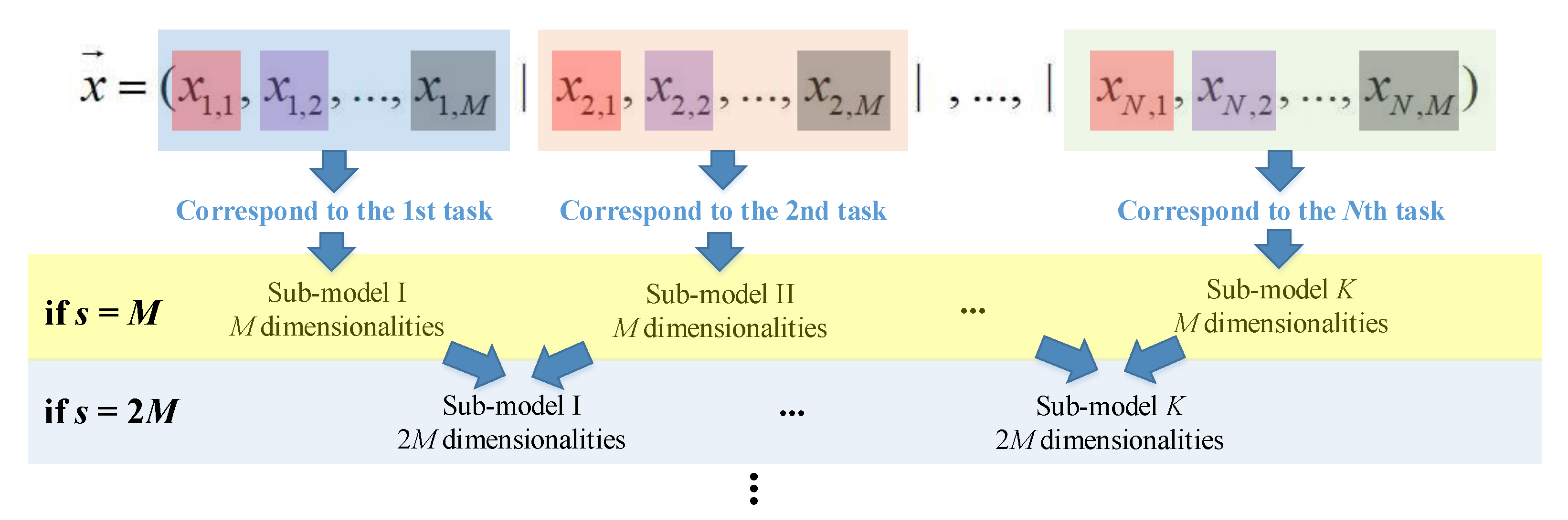
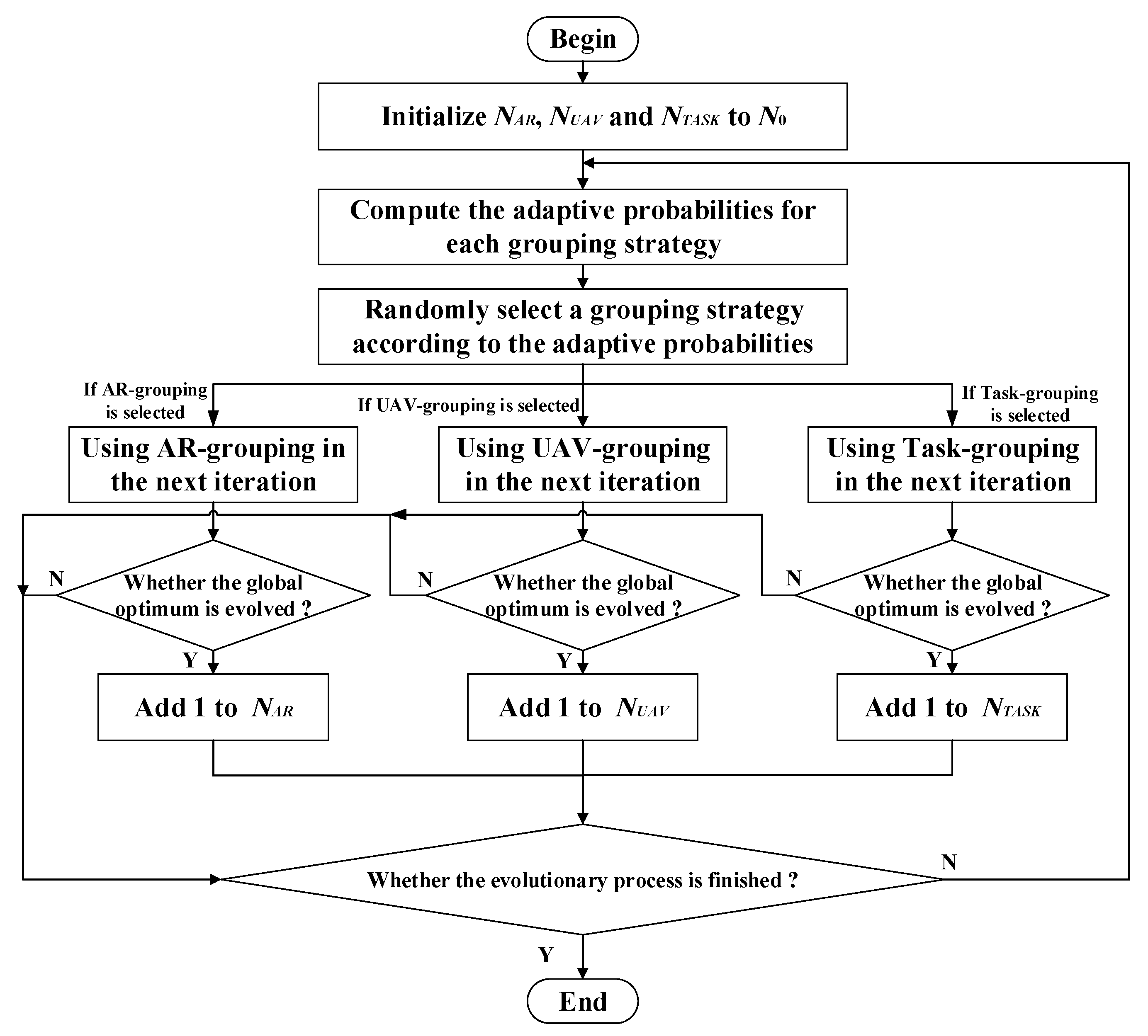
3.3. Adaptive Multiple Variable-Grouping Strategy
- (1)
- Adaptive random grouping
- (2)
- UAV variable grouping
- (3)
- Task variable grouping
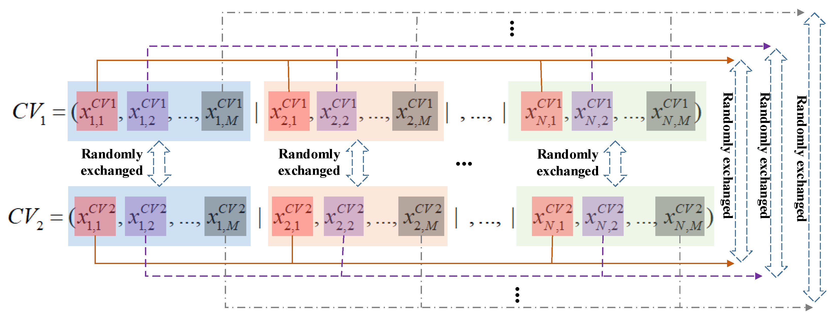
3.4. Context Vector Crossover and Mutation Strategy
- (1)
- CV crossover strategy
- (2)
- CV mutation strategy
- If , keep CVi unchanged;
- Otherwise, each of the components [xn,1, xn,2, …, xn,M] (n = 1, 2, …, N) in CVi is randomly mutated to [r0, r0, …, r0, r1], [r0, …, r0, r1, r0], …, [r0, r1, r0, …, r0] and [r1, r0, r0, …, r0], in which each r0 is randomly generated within [0, Hx/2) and each r1 is randomly generated within [Hx/2, Hx].
3.5. The Overall CCPSO-mg-cvcm Optimization Algorithm
| Algorithm 1. Pseudo code of CCPSO-mg-cvcm. |
| Initialize dimensional Population with NP particles. Initialize pcv context vectors with the best (pcv − 1) particles and a randomly selected particle. repeat Update the adaptive probabilities for each grouping strategy, and randomly select a grouping strategy according to these probabilities. Decompose the original D-dimensional model into several sub-models using the selected grouping strategy. Denote the jth sub-model as Sub-Modelj. Execute the CV crossover operation for Nmu times. Execute the mutation operation for each CV. |
| for each Sub-Modelj do |
| Coevolve the corresponding variables using AMCCPSO principles [30]. end |
| until the stopping criteria are satisfied. |
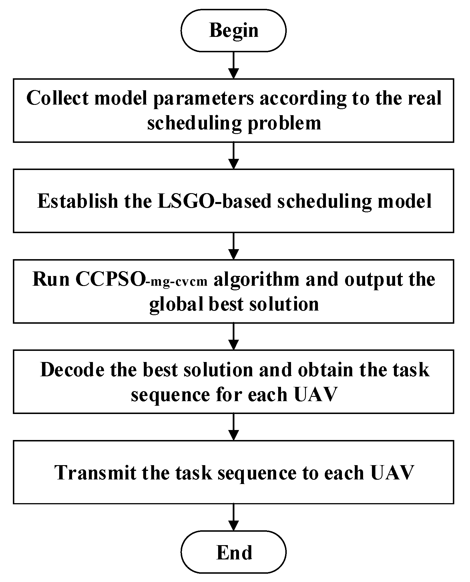
3.6. Application of the Overall UAV Swarm Scheduling Methodology
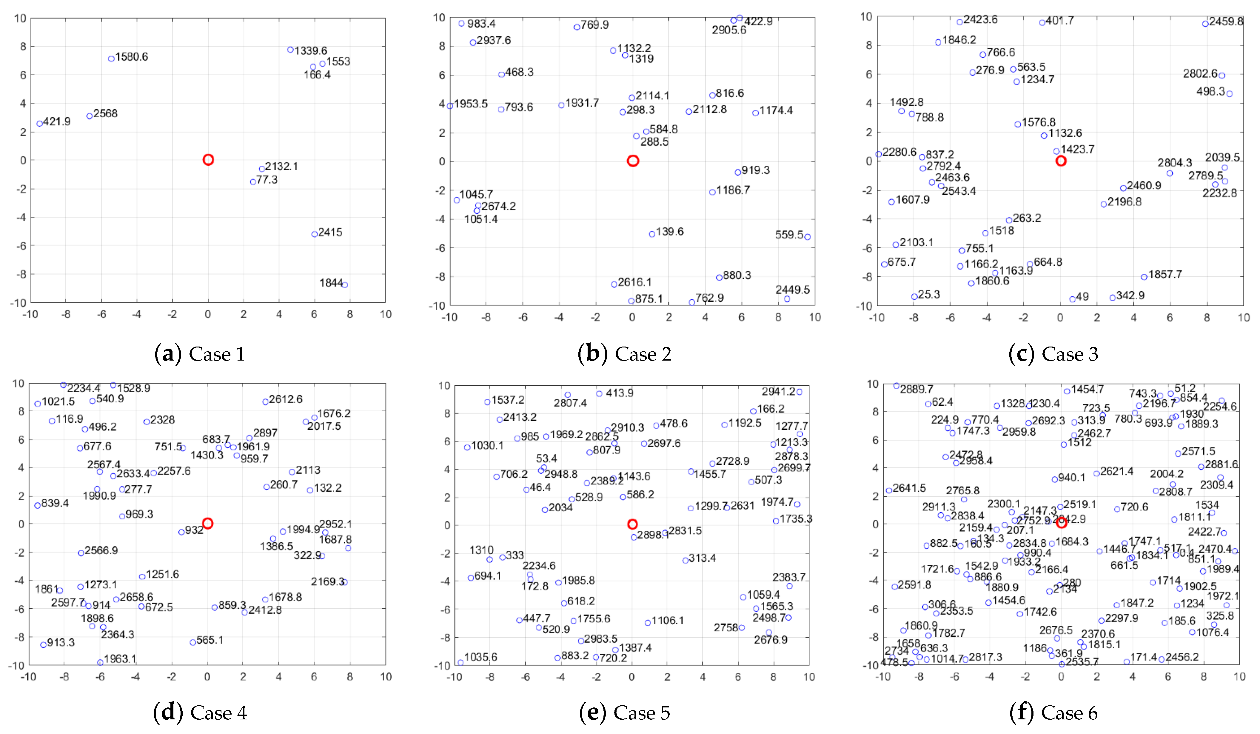
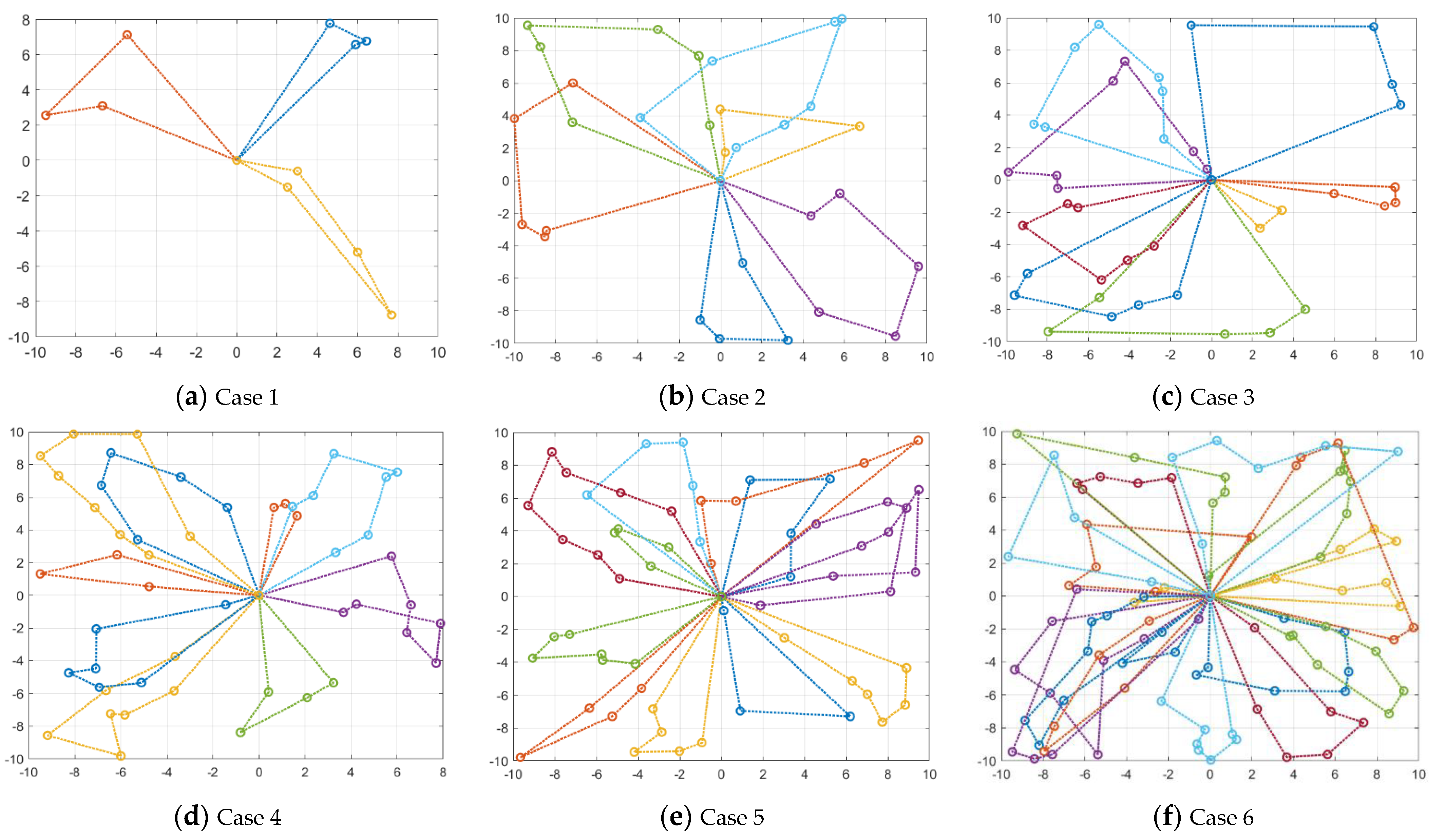
4. Case Studies and Analysis
4.1. Experimental Setup
4.2. Experimental Results and Analysis
4.3. Analysis for Different Model Dimensionalities
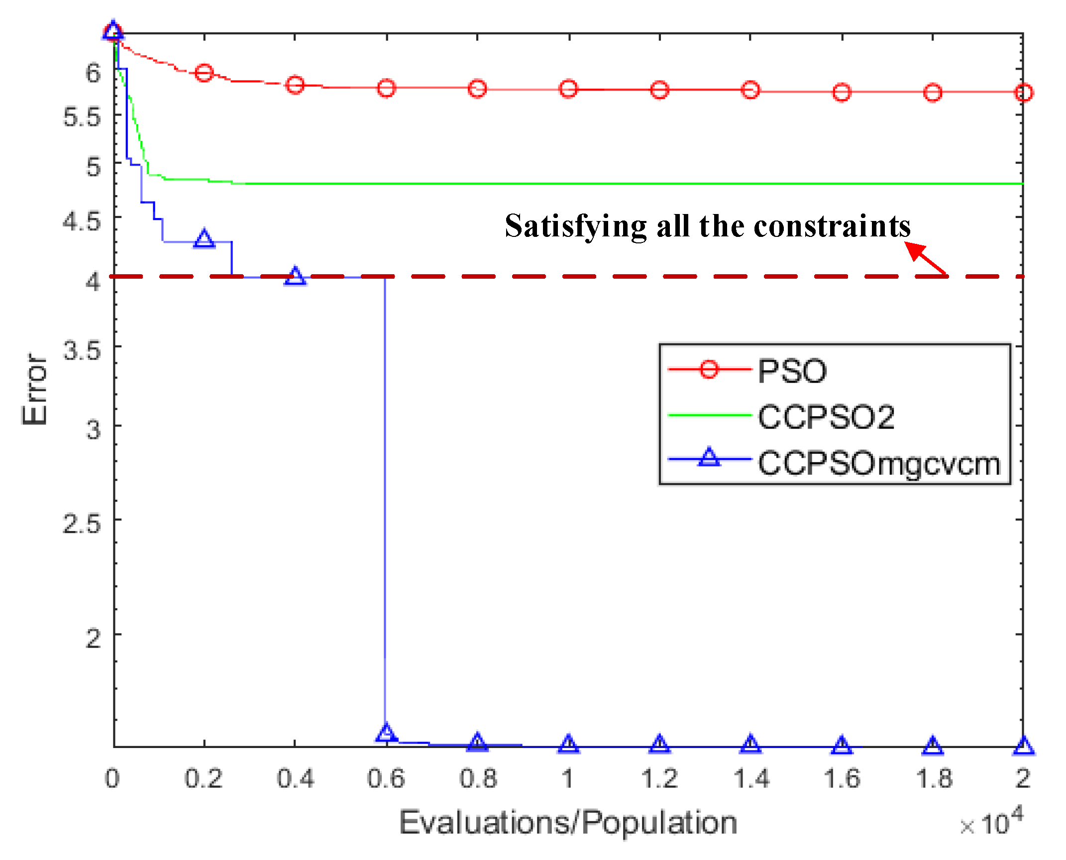
4.4. Comparison for Different Algorithms
5. Conclusions
Author Contributions
Funding
Conflicts of Interest
References
- Ivushkin, K.; Bartholomeus, H.; Bregt, A.K.; Pulatov, A.; Franceschini, M.H.D.; Kramer, H.; van Loo, E.N.; Jaramillo Roman, V.; Finkers, R. UAV based soil salinity assessment of cropland. Geoderma 2019, 338, 502–512. [Google Scholar] [CrossRef]
- Wallace, L.; Lucieer, A.; Malenovský, Z.; Turner, D.; Vopěnka, P. Assessment of forest structure using two UAV techniques: A comparison of airborne laser scanning and structure from motion (SfM) point clouds. Forests 2016, 7, 62. [Google Scholar] [CrossRef] [Green Version]
- Zhu, J.S.; Sun, K.; Jia, S.; Li, Q.Q.; Hou, X.X.; Lin, W.D.; Liu, B.Z.; Qiu, G.P. Urban Traffic Density Estimation Based on Ultrahigh-Resolution UAV Video and Deep Neural Network. IEEE J. Sel. Top. Appl. Earth Obs. Remote Sens. 2018, 11, 4968–4981. [Google Scholar] [CrossRef]
- Congress, S.S.C.; Puppala, A.J.; Lundberg, C.L. Total system error analysis of UAV-CRP technology for monitoring transportation infrastructure assets. Eng. Geol. 2018, 247, 104–116. [Google Scholar] [CrossRef]
- Liu, J.L.; Liao, X.H.; Ye, H.P.; Yue, H.Y.; Wang, Y.; Tan, X.; Wang, D.L. UAV swarm scheduling method for remote sensing observations during emergency scenarios. Remote Sens. 2022, 14, 1406. [Google Scholar] [CrossRef]
- Choi, Y.; Rayl, J.; Tammineedi, C.; Brownson, J.R.S. PV Analyst: Coupling ArcGIS with TRNSYS to assess distributed photovoltaic potential in urban areas. Sol. Energy 2011, 85, 2924–2939. [Google Scholar] [CrossRef]
- Liao, W.; Xu, S.; Heo, Y. Evaluation of model fidelity for solar analysis in the context of distributed PV integration at urban scale. Build. Simul. 2022, 15, 3–16. [Google Scholar] [CrossRef]
- Shafique, M.; Luo, X.W.; Zuo, J. Photovoltaic-green roofs: A review of benefits, limitations, and trends. Solar Energy 2020, 202, 485–497. [Google Scholar] [CrossRef]
- Hwang, Y.S.; Schluter, S.; Park, S.I.; Um, J.S. Comparative evaluation of mapping accuracy between UAV video versus photo mosaic for the scattered urban photovoltaic panel. Remote Sens. 2021, 13, 2745. [Google Scholar] [CrossRef]
- Niccolai, A.; Grimaccia, F.; Leva, S. Advanced asset management tools in photovoltaic plant monitoring: UAV-based digital mapping. Energies 2019, 12, 4736. [Google Scholar] [CrossRef] [Green Version]
- Li, X.X.; Yang, Q.; Chen, Z.B.; Luo, X.J.; Yan, W.J. Visible defects detection based on UAV-based inspection in large-scale photovoltaic systems. IET Renew. Power Gener. 2017, 11, 1234–1244. [Google Scholar] [CrossRef]
- Gu, Z.; Yin, T.T.; Ding, Z.T. Path tracking control of autonomous vehicles subject to deception attacks via a learning-based event-triggered mechanism. IEEE Trans. Neural Netw. Learn. Syst. 2021, 32, 5644–5653. [Google Scholar] [CrossRef] [PubMed]
- Niu, Z.C.; Liu, H.; Lin, X.M.; Du, J.Z. Task scheduling with UAV-assisted dispersed computing for disaster scenario. IEEE Syst. J. 2022, 1–12. [Google Scholar] [CrossRef]
- Hanna, S.; Krijestorac, E.; Cabric, D. UAV swarm position optimization for high capacity MIMO backhaul. IEEE J. Sel. Areas Commun. 2021, 39, 3006–3021. [Google Scholar] [CrossRef]
- Phung, M.D.; Ha, Q.P. Safety-enhanced UAV path planning with spherical vector-based particle swarm optimization. Appl. Soft Comput. 2021, 107, 107376. [Google Scholar] [CrossRef]
- Wang, S.F.; Zhou, J.; Zhong, H.L. Estimating land surface temperature from satellite passive microwave observations with the traditional neural network, deep belief network, and convolutional neural network. Remote Sens. 2020, 12, 2691. [Google Scholar] [CrossRef]
- Chang, Y.L.; Tan, T.H.; Lee, W.H.; Chang, L.A.; Chen, Y.N.; Fan, K.C.; Alkhaleefah, M. Consolidated convolutional neural network for hyperspectral image classification. Remote Sens. 2022, 14, 1571. [Google Scholar] [CrossRef]
- Tang, R.L.; Wu, Z.; Li, X. Optimal operation of photovoltaic/battery/diesel/cold-ironing hybrid energy system for maritime application. Energy 2018, 162, 697–714. [Google Scholar] [CrossRef]
- An, Q.; Chen, X.; Wang, H.; Yang, H.; Yang, Y. Segmentation of concrete cracks by using fractal dimension and UHK-net. Fractal Fract. 2022, 6, 95. [Google Scholar] [CrossRef]
- An, Q.; Chen, X.J.; Zhang, J.Q.; Shi, R.Z.; Yang, Y.J.; Huang, W. A robust fire detection model via convolution neural networks for intelligent robot vision sensing. Sensors 2022, 22, 2929. [Google Scholar] [CrossRef]
- Liu, H.; Nie, H.; Zhang, Z.; Li, Y.-F. Anisotropic angle distribution learning for head pose estimation and attention understanding in hu-man-computer interaction. Neurocomputing 2021, 433, 310–322. [Google Scholar] [CrossRef]
- Gu, Z.; Ahn, C.K.; Yan, S.; Xie, X.P.; Yue, D. Event-triggered filter design based on average measurement output for networked unmanned surface vehicles. IEEE Trans. Circuits Syst. II Express Briefs 2022. [Google Scholar] [CrossRef]
- Liu, H.; Zheng, C.; Li, D.; Zhang, Z.; Lin, K.; Shen, X.; Xiong, N.N.; Wang, J. Multi-perspective social recommendation method with graph representation learning. Neurocomputing 2022, 468, 469–481. [Google Scholar] [CrossRef]
- Shaikh, P.W.; El-Abd, M.; Khanafer, M.; Gao, K.Z. A review on swarm intelligence and evolutionary algorithms for solving the traffic signal control problem. IEEE Trans. Intell. Transp. Syst. 2022, 23, 48–63. [Google Scholar] [CrossRef]
- Li, X.T.; Ma, S.J.; Hu, J.H. Multi-search differential evolution algorithm. Appl. Intell. 2017, 47, 231–256. [Google Scholar] [CrossRef]
- Zhong, X.X.; Cheng, P. An elite-guided hierarchical differential evolution algorithm. Appl. Intell. 2021, 51, 4962–4983. [Google Scholar] [CrossRef]
- Chen, X.; Tianfield, H.; Du, W.L. Bee-foraging learning particle swarm optimization. Appl. Soft Comput. 2021, 102, 107134. [Google Scholar] [CrossRef]
- Tang, R.L.; Li, X.; Lai, J.G. A novel optimal energy-management strategy for a maritime hybrid energy system based on large-scale global optimization. Appl. Energy 2018, 228, 254–264. [Google Scholar] [CrossRef]
- Li, X.D.; Yao, X. Cooperatively coevolving particle swarms for large-scale optimization. IEEE Trans. Evol. Comput. 2012, 16, 210–224. [Google Scholar]
- Tang, R.L.; Wu, Z.; Fang, Y.J. Adaptive multi-context cooperatively coevolving particle swarm optimization for large-scale problems. Soft Comput. 2017, 21, 4735–4754. [Google Scholar] [CrossRef]
- Li, X.D.; Yao, X. Tackling high dimensional nonseparable optimization problems by cooperatively coevolving particle swarms. In Proceedings of the 2009 IEEE Congress on Evolutionary Computation, Trondheim, Norway, 18–21 May 2009; pp. 1546–1553. [Google Scholar]
- Zhang, J.Q.; Sanderson, A.C. JADE: Adaptive differential evolution with optional external archive. IEEE Trans. Evol. Comput. 2009, 13, 945–958. [Google Scholar] [CrossRef]
- Tang, R.L.; Li, X. Adaptive multi-context cooperatively coevolving in differential evolution. Appl. Intell. 2018, 48, 2719–2729. [Google Scholar] [CrossRef]
- Liu, H.; Liu, T.; Zhang, Z.; Sangaiah, A.K.; Yang, B.; Li, Y.F. ARHPE: Asymmetric Relation-aware Representation Learning for Head Pose Estimation in Industrial Hu-man-computer Interaction. IEEE Trans. Ind. Inf. 2022. [Google Scholar] [CrossRef]


| Parameter | Meaning | Value | Parameter | Meaning | Value |
|---|---|---|---|---|---|
| vf | Speed of UAV from one UDPA to another | 25 m/s | vm | Speed of UAV when hover around PV array | 15 m/s |
| Ld-max | Maximum distance duration for each UAV | 40 km | Power consumption coefficient for UAV | 90% | |
| Hx | Upper bound of optimization variables | 100 | Penalty strength coefficient | 10,000 | |
| Step-size for random grouping | 5 | s0 | Initial group size for random grouping | 10 | |
| pcv | Number of CV | 5 | N0 | Initial value for probability coefficients | 5 |
| Np | Number of particle in the PSO swarm | 50 | Mutation probability control coefficient | 0.7 | |
| Max_ges | Maximum evaluation number for CCPSO-mg-cvcm | 2 × 10⁶ | Nmu | Number of CV crossover operation | 5 |
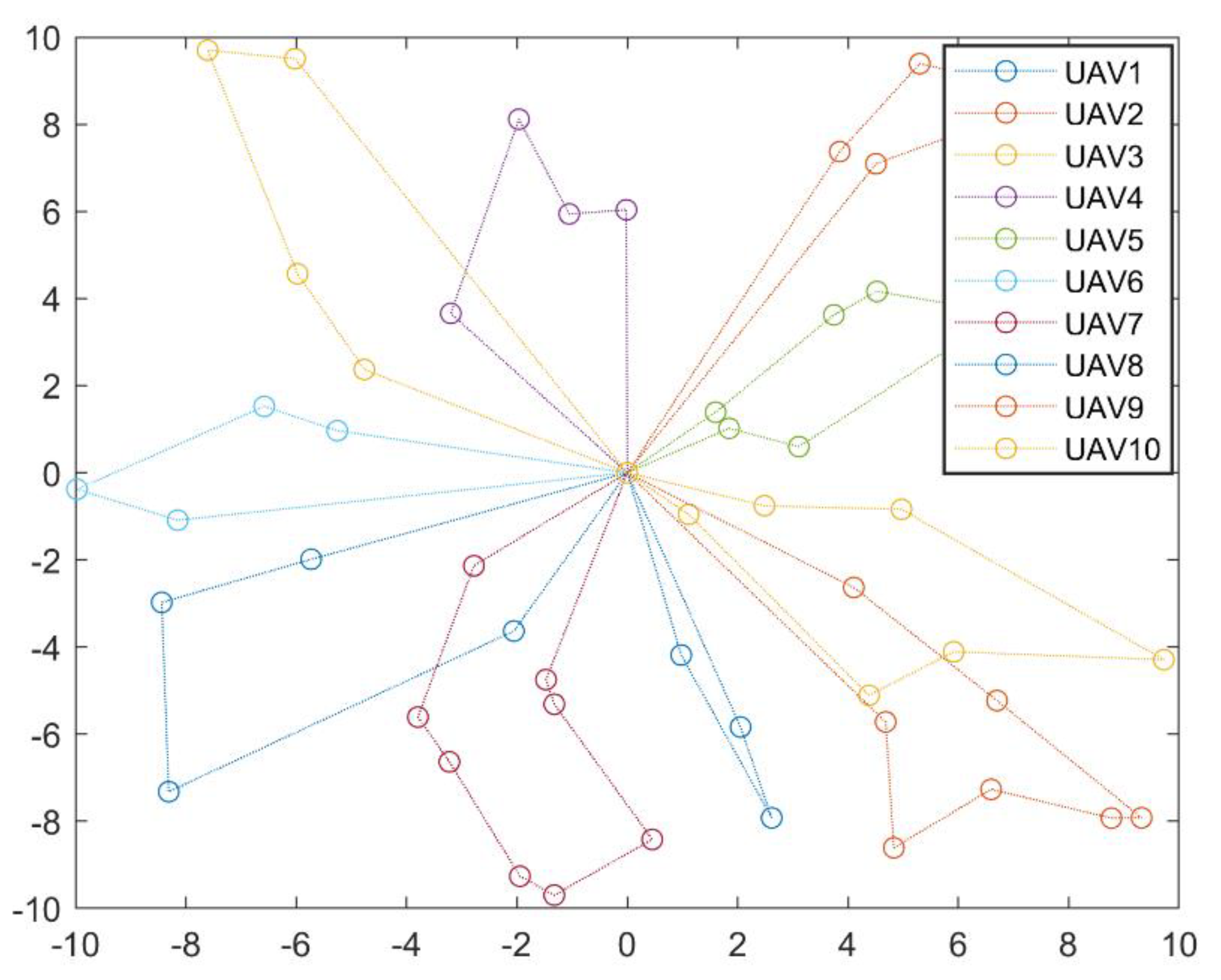
| UAV | Task Queue | UAV | Task Queue |
|---|---|---|---|
| UAV1 | 8----20----41----39 | UAV6 | 11----40----23----13 |
| UAV2 | 35----25----47----37 | UAV7 | 5----48----45----14----6----44----33----10 |
| UAV3 | 31----7----24----21----15----26 | UAV8 | 50----2----1 |
| UAV4 | 38----30----34----27 | UAV9 | 49----29----4----3----42----43----9 |
| UAV5 | 19----16----12----32----36----22 | UAV10 | 17----28----18----46 |
| Algorithm | Final Fitness Function Value | Algorithm | Final Fitness Function Value | Algorithm | Final Fitness Function Value |
|---|---|---|---|---|---|
| PSO | 547,478.43 | CCPSO2 | 64,563.43 | CCPSO-mg-cvcm | 40.45 |
| Cases | Number of UAV | Number of UDPA | Model Dimensionality | Maximum Evaluation Number |
|---|---|---|---|---|
| Case 1 | 3 | 10 | 30 | 2 × 10⁵ |
| Case 2 | 6 | 30 | 180 | 5 × 10⁵ |
| Case 3 | 8 | 40 | 320 | 1 × 10⁶ |
| Case 4 | 10 | 50 | 500 | 1 × 10⁶ |
| Case 5 | 14 | 80 | 1120 | 1 × 10⁶ |
| Case 6 | 20 | 120 | 2400 | 1 × 10⁶ |
| UAV | Task Queue | UAV | Task Queue |
|---|---|---|---|
| UAV1 | 25----27----40----50----58----93----95 | UAV11 | / |
| UAV2 | 43----44----74----80----89 | UAV12 | 13----47----49----69----70 |
| UAV3 | 18----36----45 | UAV13 | 23----53----76----81 |
| UAV4 | 8----29----39----78----83----87 | UAV14 | 6----9----10----32----48----68 |
| UAV5 | 7----24----30----37----61----94----98 | UAV15 | 2----15----51----77----85----91----99 |
| UAV6 | 31----34----35----46----66----73----96 | UAV16 | 5----19----52----57----88 |
| UAV7 | 16----33----38----72----79 | UAV17 | 11----26----28----63 |
| UAV8 | 1----14----67 | UAV18 | 22----54----55----75----90 |
| UAV9 | 59----62----64----86----100 | UAV19 | 3----17----20----41----71----82----84 |
| UAV10 | 12----21----56 | UAV20 | 4----42----60----65----92----97 |
| Cases | Number of UAV | Number of UDPA | Model Dimensionality | Maximum Evaluation Number |
|---|---|---|---|---|
| Case 7 | 6 | 30 | 180 | 1 × 10⁶ |
| Case 8 | 12 | 60 | 720 | 1 × 10⁶ |
| Case 9 | 15 | 80 | 1200 | 1 × 10⁶ |
| Case 10 | 20 | 100 | 2000 | 1 × 10⁶ |
| Cases | CPSO-SK-rg-aw | CCPSO2 | JADE | AMCCDE | CCPSO-mg-cvcm |
|---|---|---|---|---|---|
| Case 7 | 7.2602 × 10⁴ | 2.9142 × 101 | 1.6330 × 10⁴ | 2.7599 × 101 | 2.5251 × 101 |
| Case 8 | 1.3087 × 10⁵ | 6.8420 × 10⁴ | 7.4197 × 10⁵ | 3.3308 × 10⁴ | 4.3747 × 101 |
| Case 9 | 2.3357 × 10⁵ | 1.0856 × 10⁵ | 1.8142 × 10⁶ | 8.4918 × 10⁴ | 6.1996 × 101 |
| Case 10 | 3.3947 × 10⁵ | 1.3128 × 10⁵ | 4.4930 × 10⁶ | 9.4073 × 10⁴ | 8.0628 × 101 |
Publisher’s Note: MDPI stays neutral with regard to jurisdictional claims in published maps and institutional affiliations. |
© 2022 by the authors. Licensee MDPI, Basel, Switzerland. This article is an open access article distributed under the terms and conditions of the Creative Commons Attribution (CC BY) license (https://creativecommons.org/licenses/by/4.0/).
Share and Cite
An, Q.; Hu, Q.; Tang, R.; Rao, L. Intelligent Scheduling Methodology for UAV Swarm Remote Sensing in Distributed Photovoltaic Array Maintenance. Sensors 2022, 22, 4467. https://doi.org/10.3390/s22124467
An Q, Hu Q, Tang R, Rao L. Intelligent Scheduling Methodology for UAV Swarm Remote Sensing in Distributed Photovoltaic Array Maintenance. Sensors. 2022; 22(12):4467. https://doi.org/10.3390/s22124467
Chicago/Turabian StyleAn, Qing, Qiqi Hu, Ruoli Tang, and Lang Rao. 2022. "Intelligent Scheduling Methodology for UAV Swarm Remote Sensing in Distributed Photovoltaic Array Maintenance" Sensors 22, no. 12: 4467. https://doi.org/10.3390/s22124467