
Fast Transmitarray Synthesis with Far-Field and Near-Field Constraints


Abstract
:1. Introduction
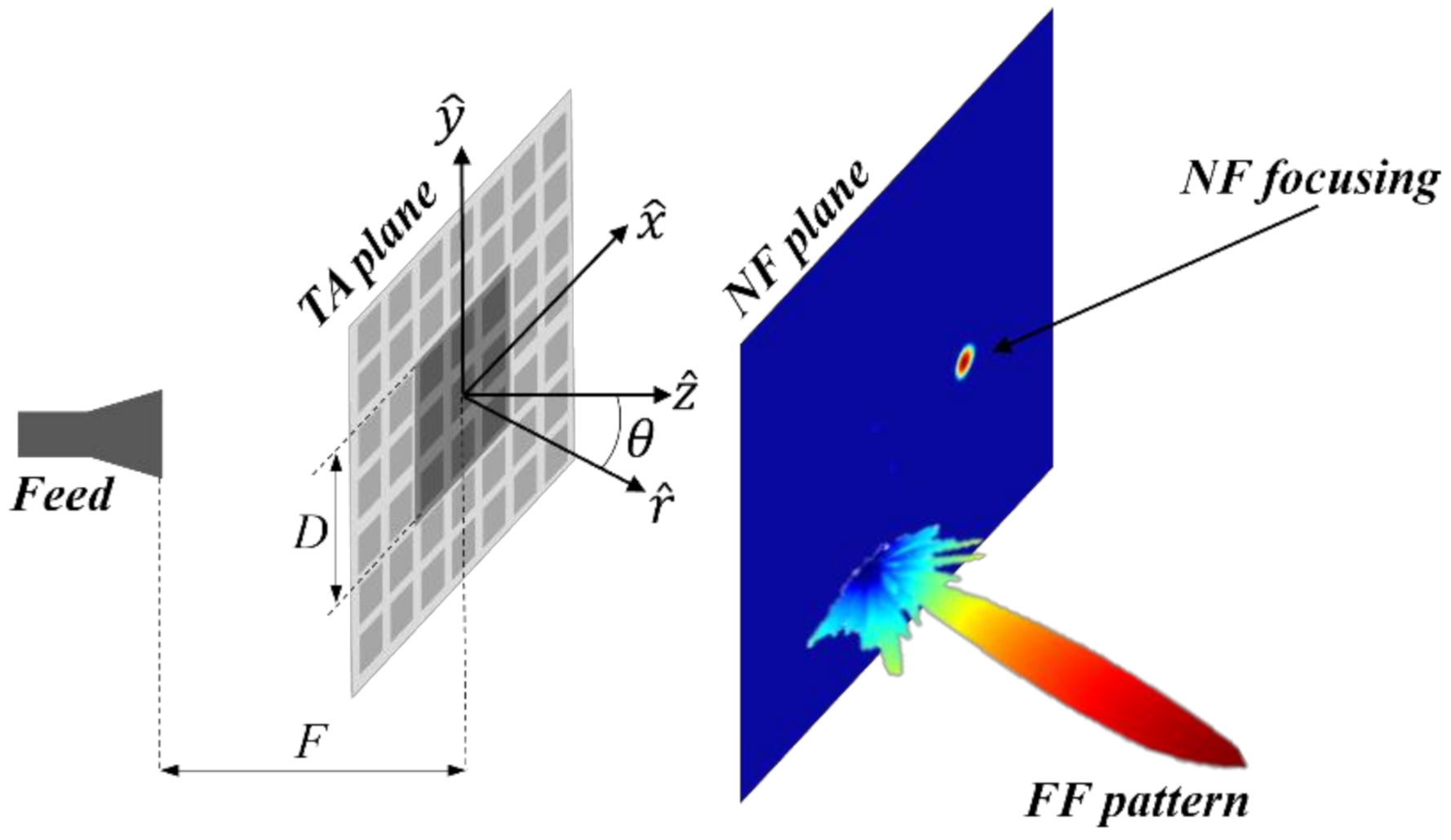
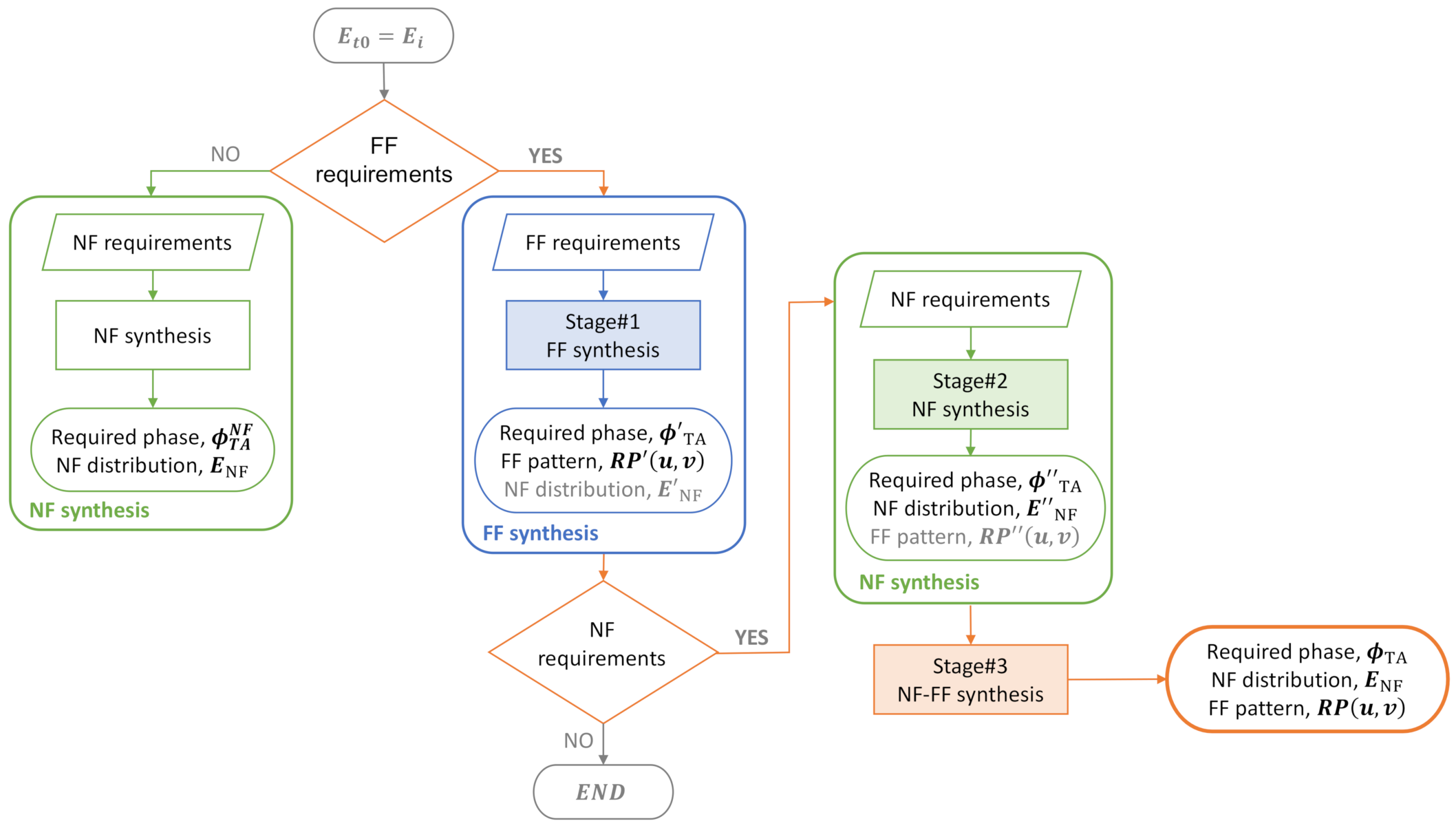
2. Methodology
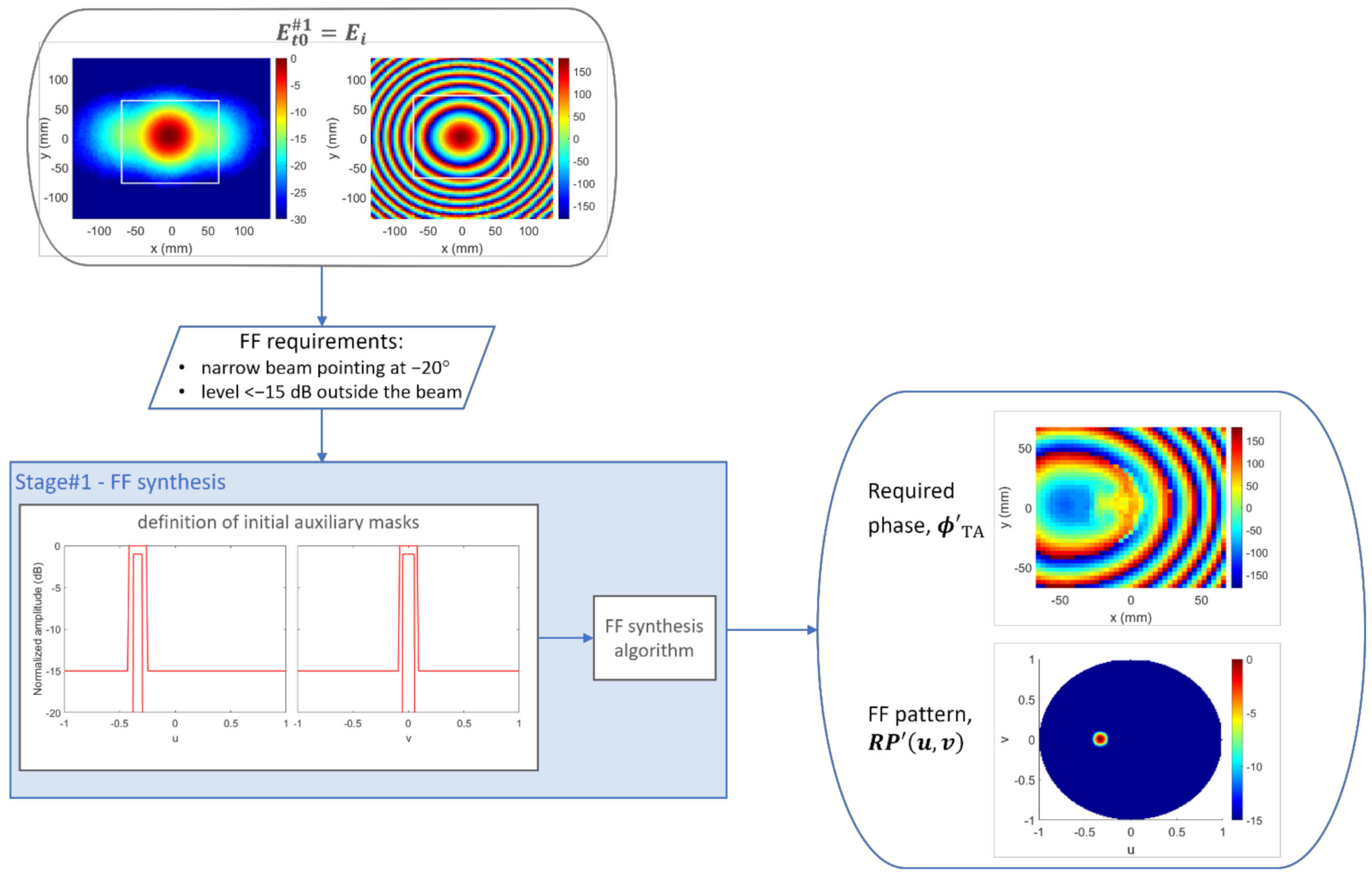
- Stage#1: only FF constraints are considered to perform the FF synthesis algorithm described in [21,23]. These constraints concern the pointing direction, beamwidth, and secondary lobe level (SLL). From these specifications, upper () and lower () auxiliary templates are defined.To initialize the algorithm, the TA is supposed to be transparent; hence, the initial electric field transmitted to the other side of the TA () is the field incident from the feeding source (), given by Equation (1).As a result of the synthesis, the matrix of the necessary phase shifts () to be introduced by the TA in order to get a radiation pattern () that complies with the specifications (FF requirements) is obtained.
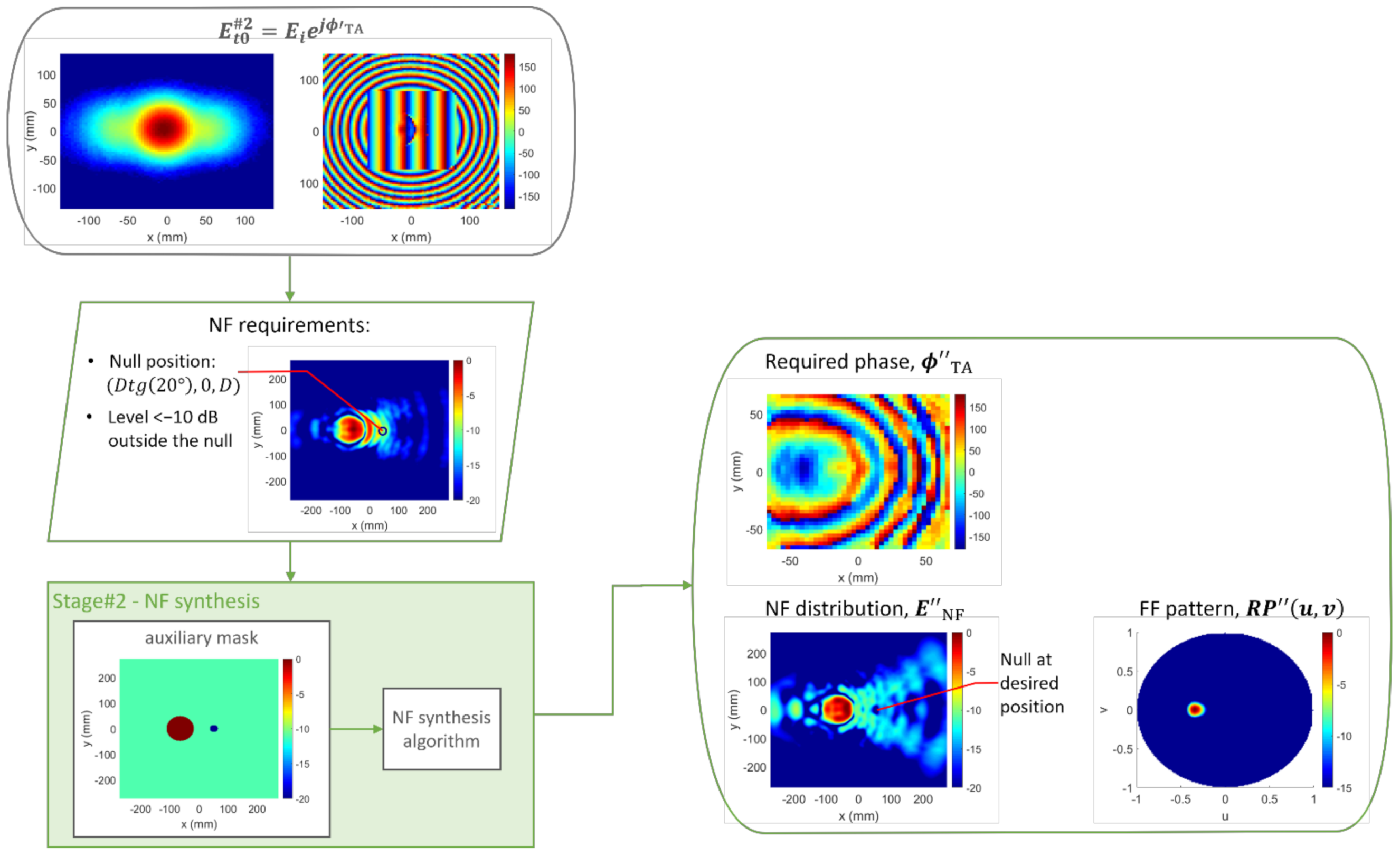
- Stage#2: only NF constraints are considered to perform the NF synthesis algorithm described in [22] (there is a typo in Figure 2 of reference [22]: according to (4) should read according to (3)). NF requirements may include the position of the focus spot or the NF null, as appropriate, as well as the spot width and SLL. From these specifications, upper () and lower () auxiliary templates are defined.In this case, the starting point for the algorithm is the phases resulting from Stage#1. Therefore, the field initially transmitted to the other side of the TA is expressed asAs a result of the synthesis, the matrix of the necessary phase shifts () to be introduced by the TA in order to get a field distribution on the near region () that complies with the specifications (NF requirements) is obtained. With these new values of the transmission coefficient phase, the FF pattern becomes .
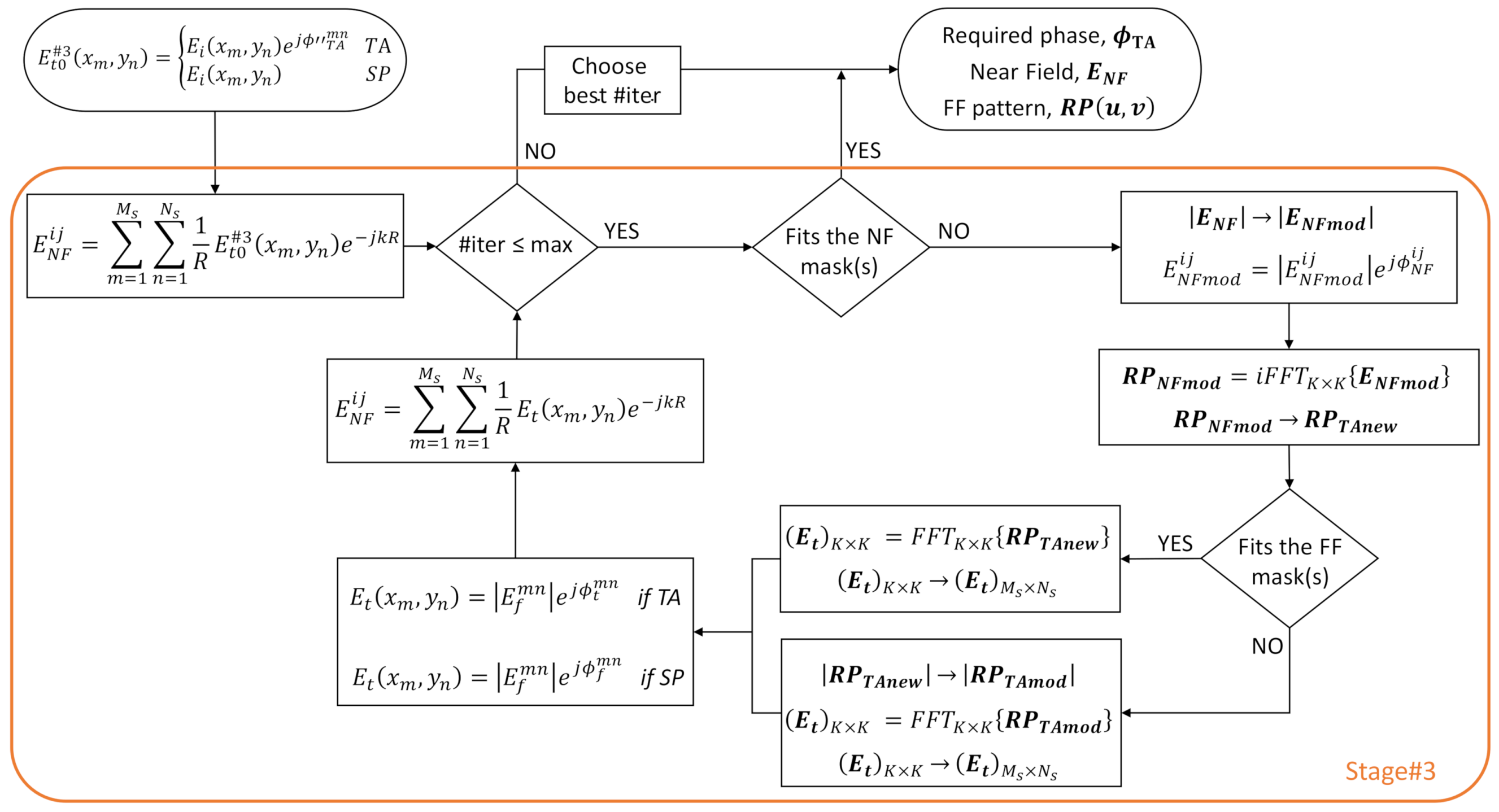
- Stage#3: the above two constraints are merged to take into account both the NF and FF constrains.The starting point for the algorithm is now the phases resulting from Stage#2. Therefore, the field initially transmitted to the other side of the TA () is expressed as shown in Equation (3), changing to .As a result of the synthesis, the matrix of the necessary phase shifts () to be introduced by the TA in order to get a field distribution in the near region () that complies with NF constraints and a radiation pattern () that complies with FF constraints is obtained.
3. Results of the Synthesis Algorithm and Experimental Validation
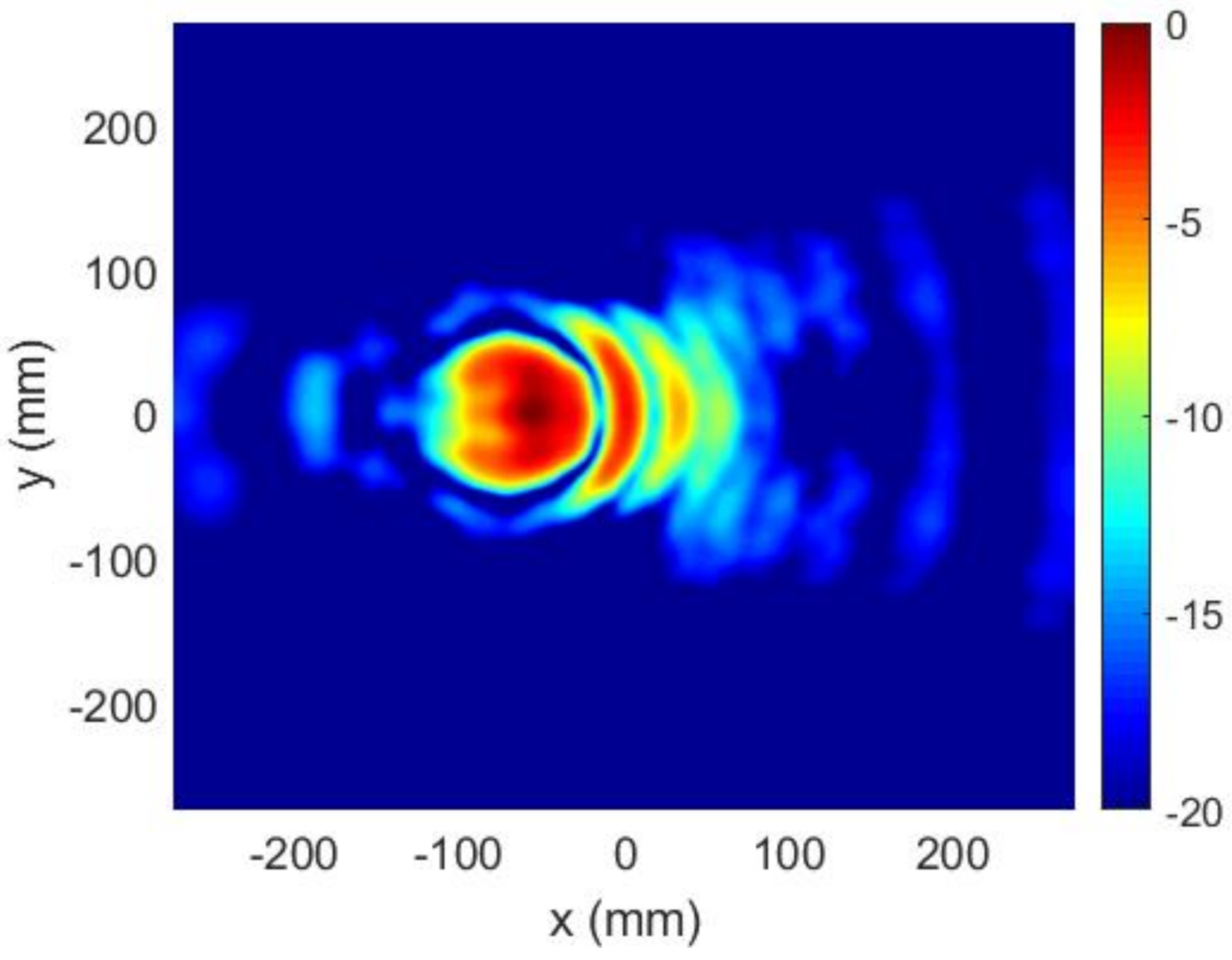
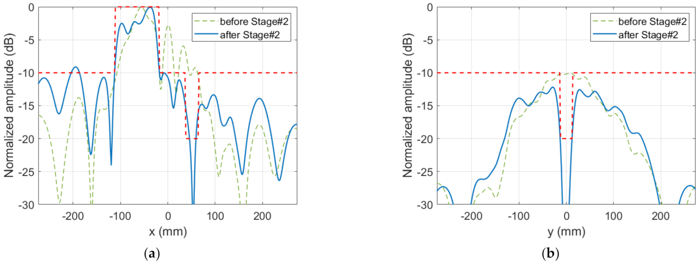
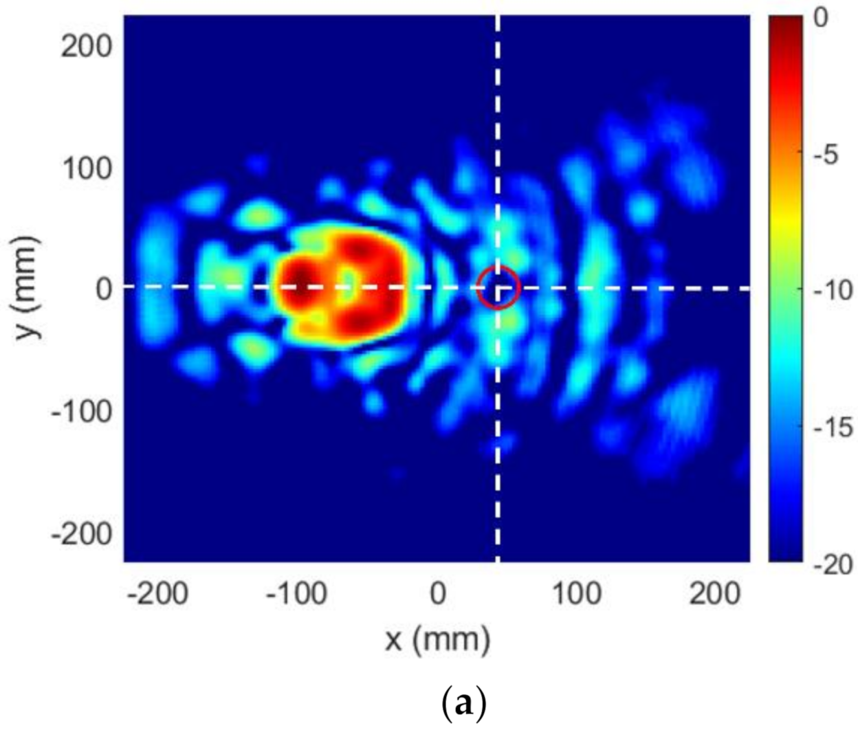
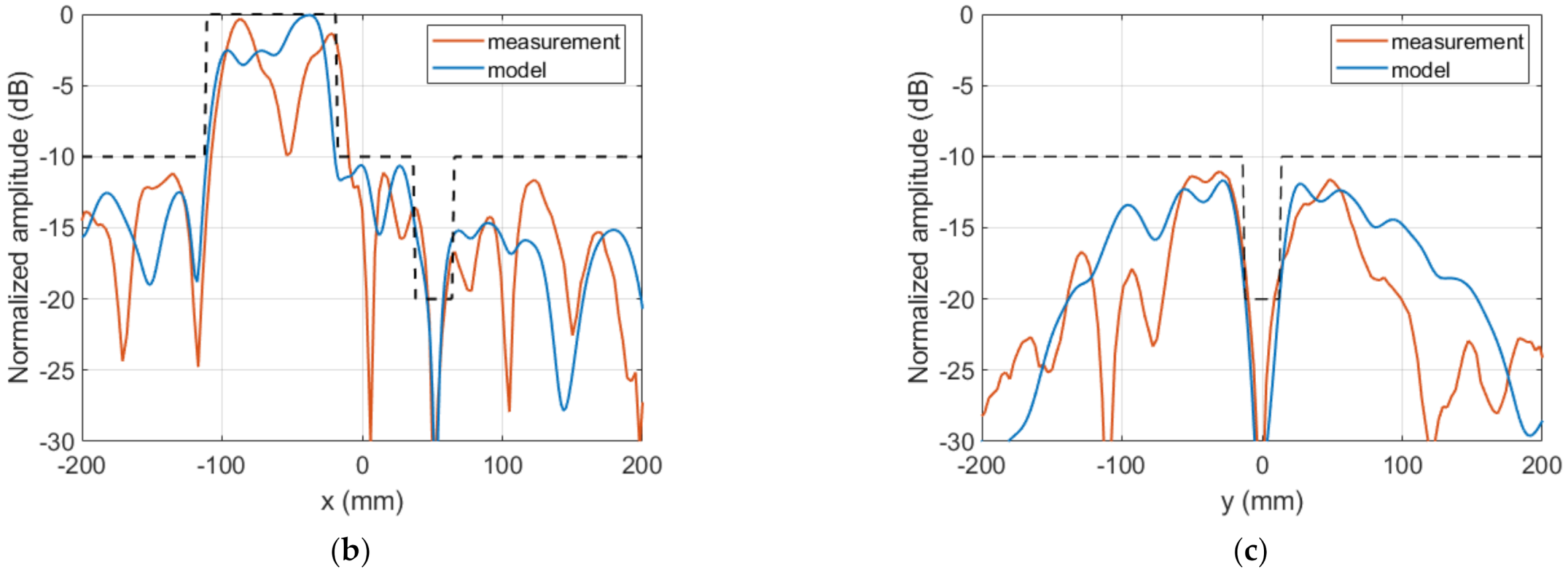
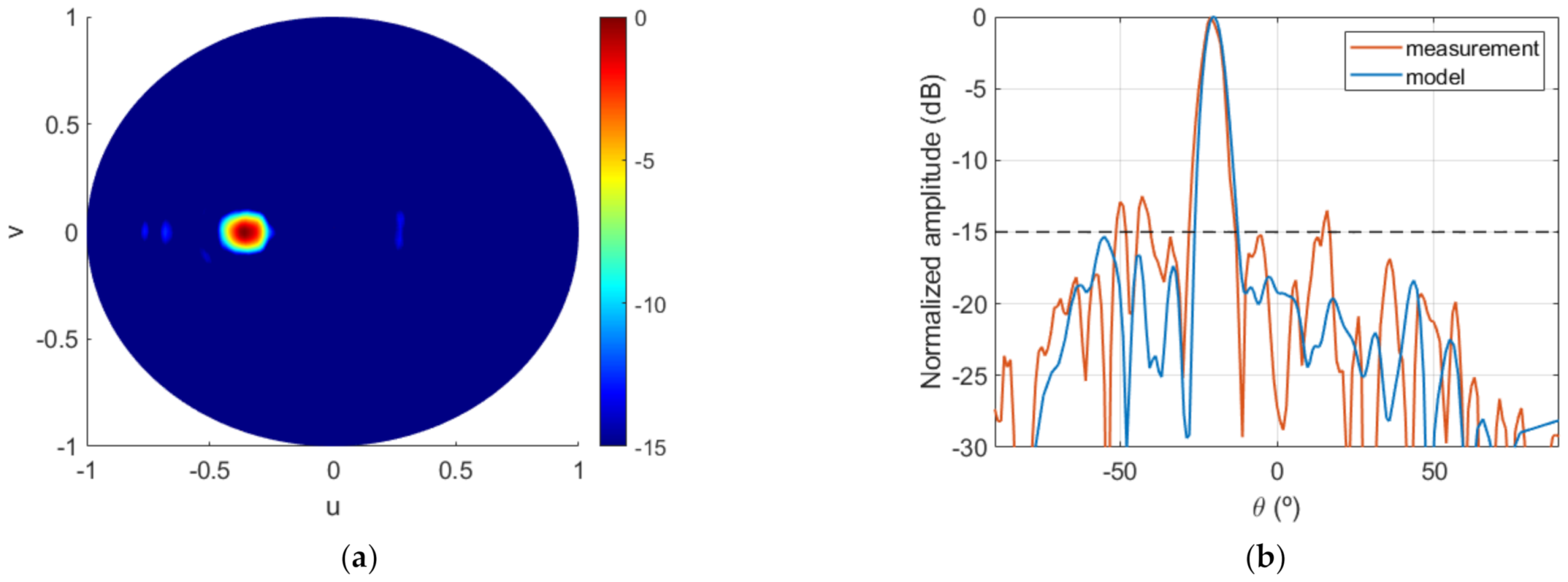
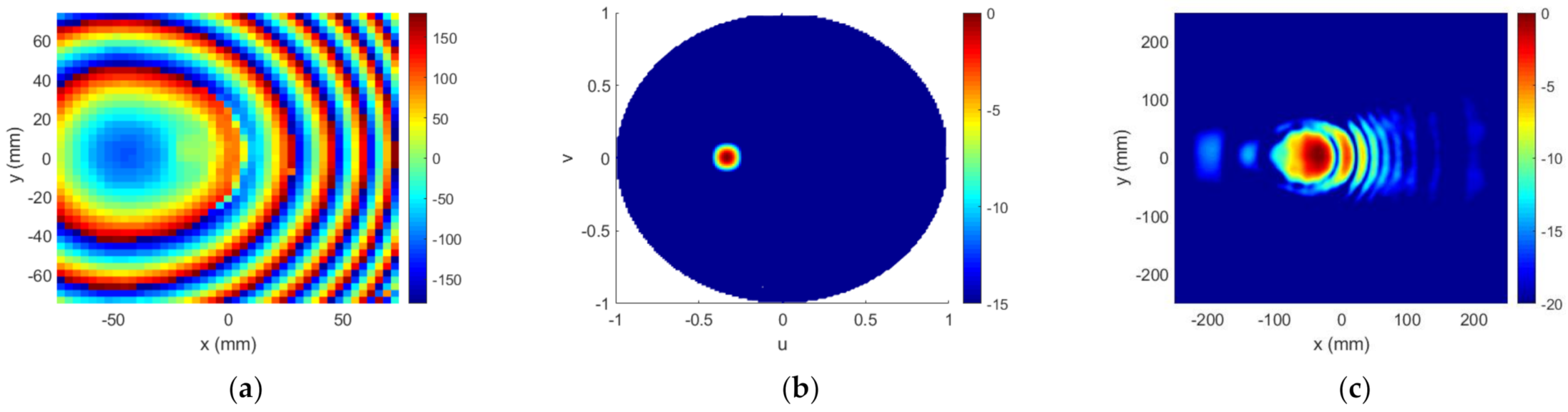
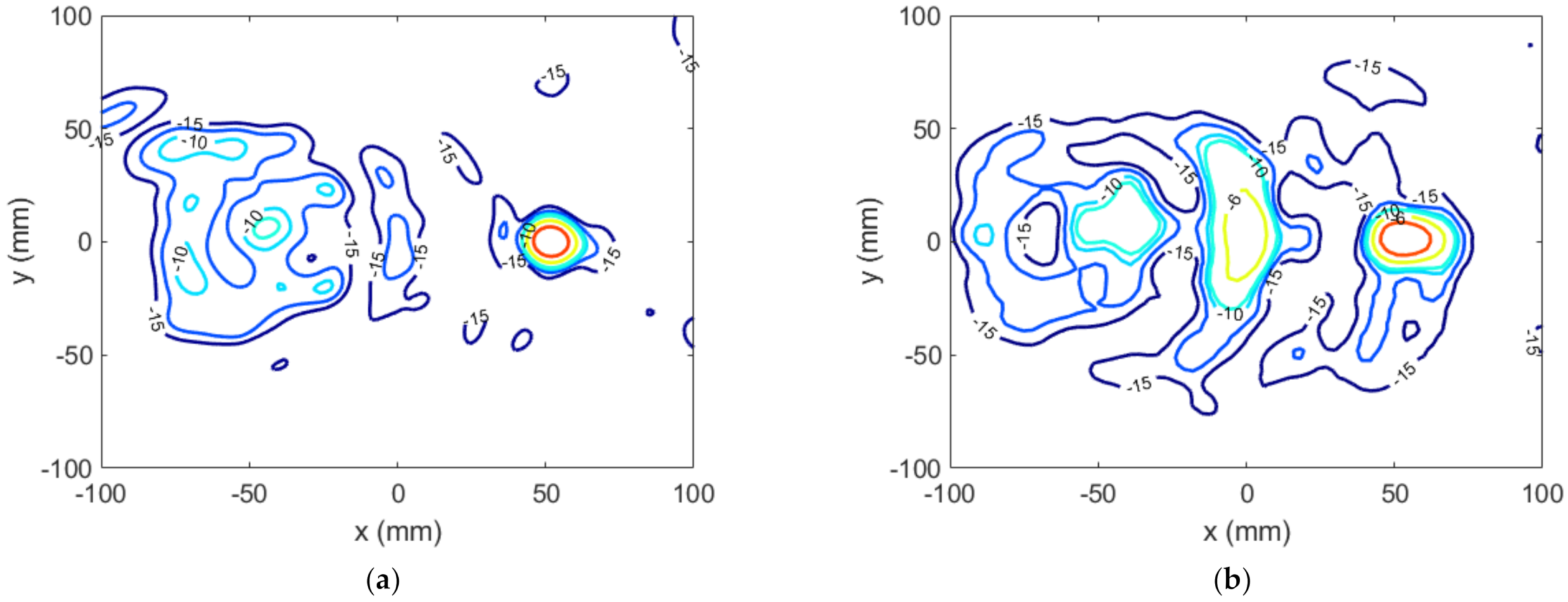
3.1. Case 1: Far-Field Beam and Null in Near Field
- FF: pointing at with SLL lower than −15 dB outside the main lobe.
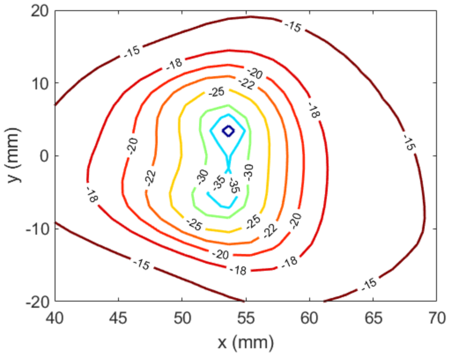
- NF: null at the position , with , and level lower than −10 dB for all other directions except that of the FF beam.
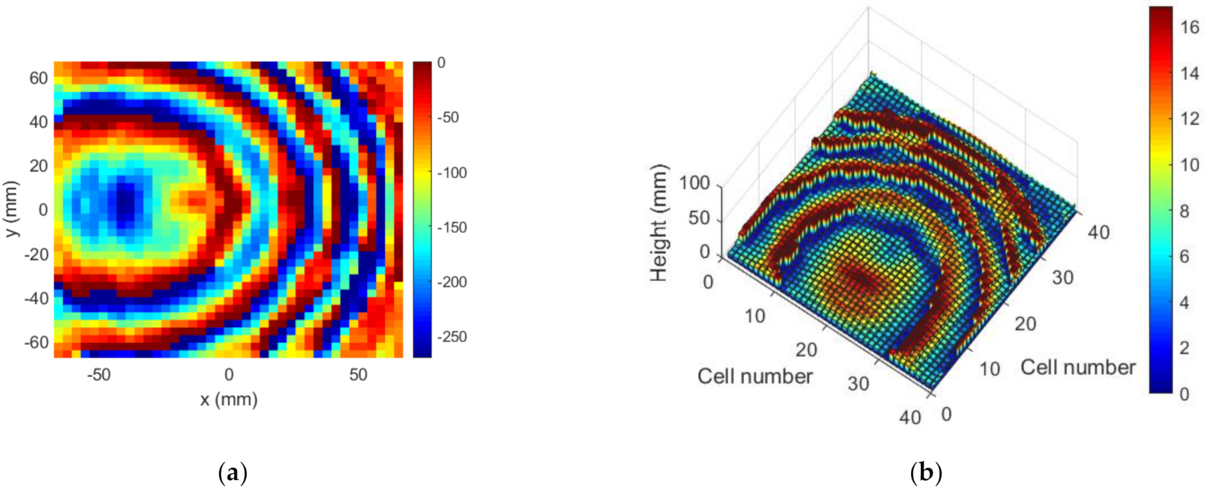
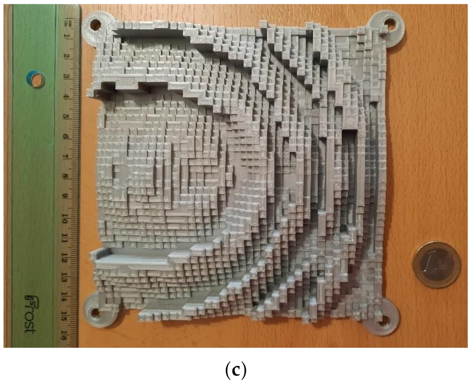
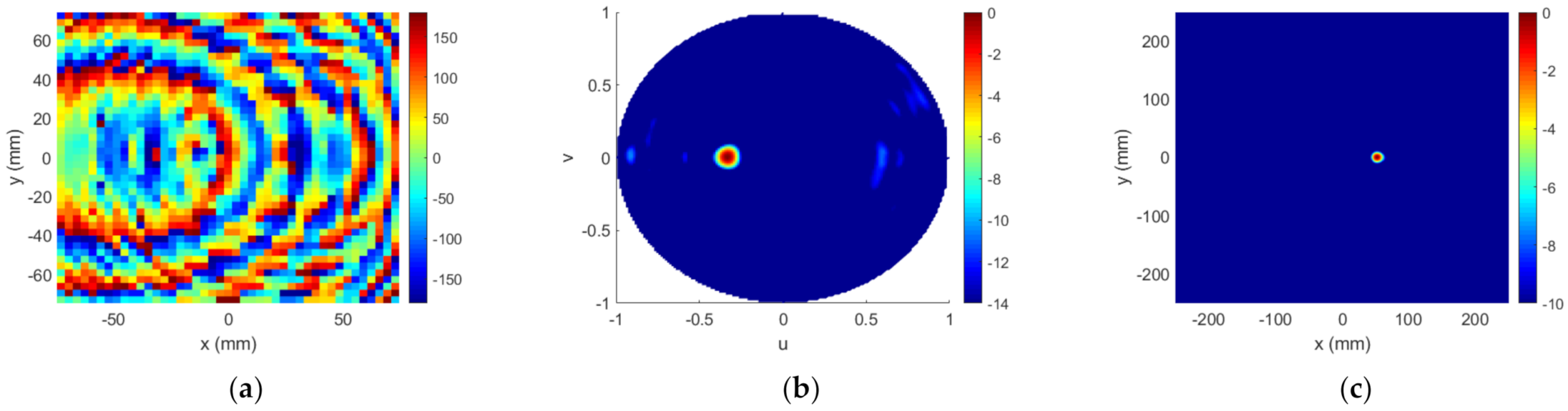
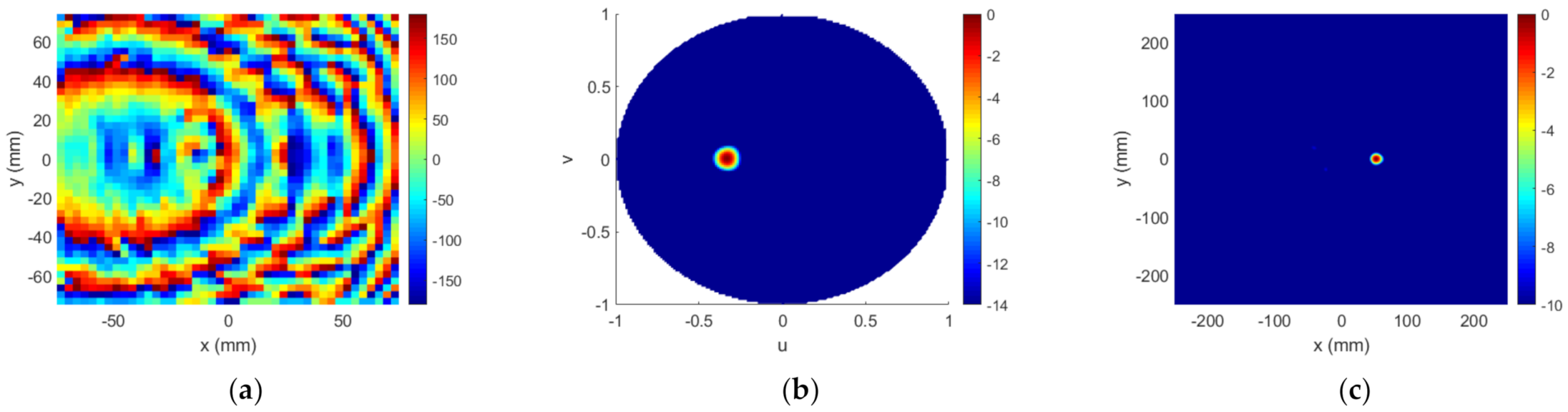
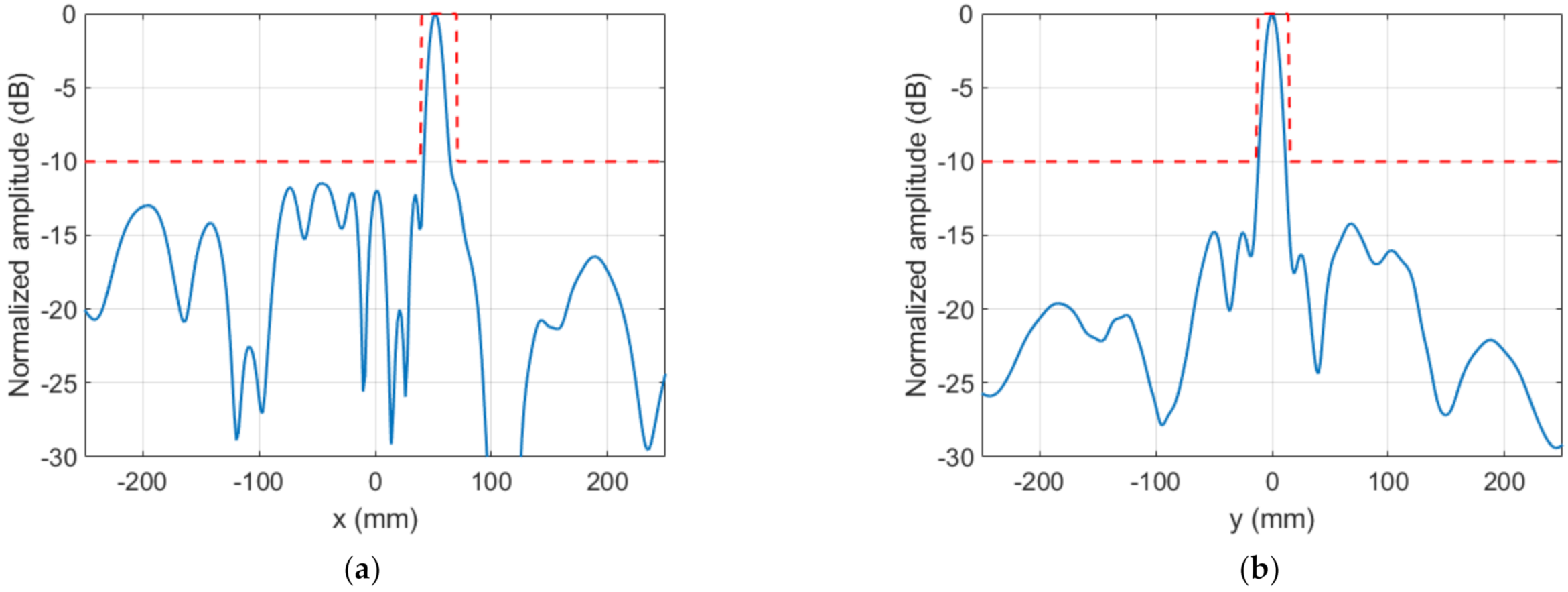
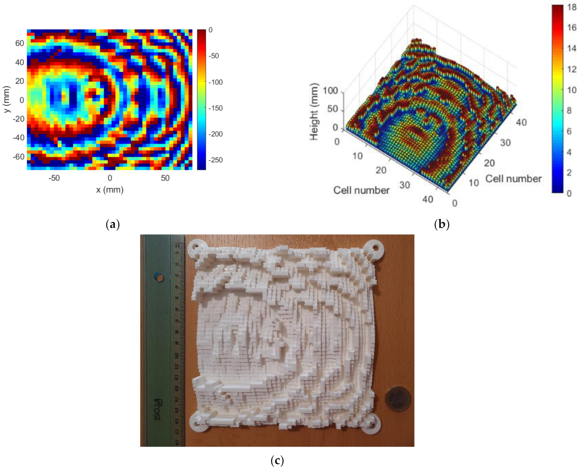
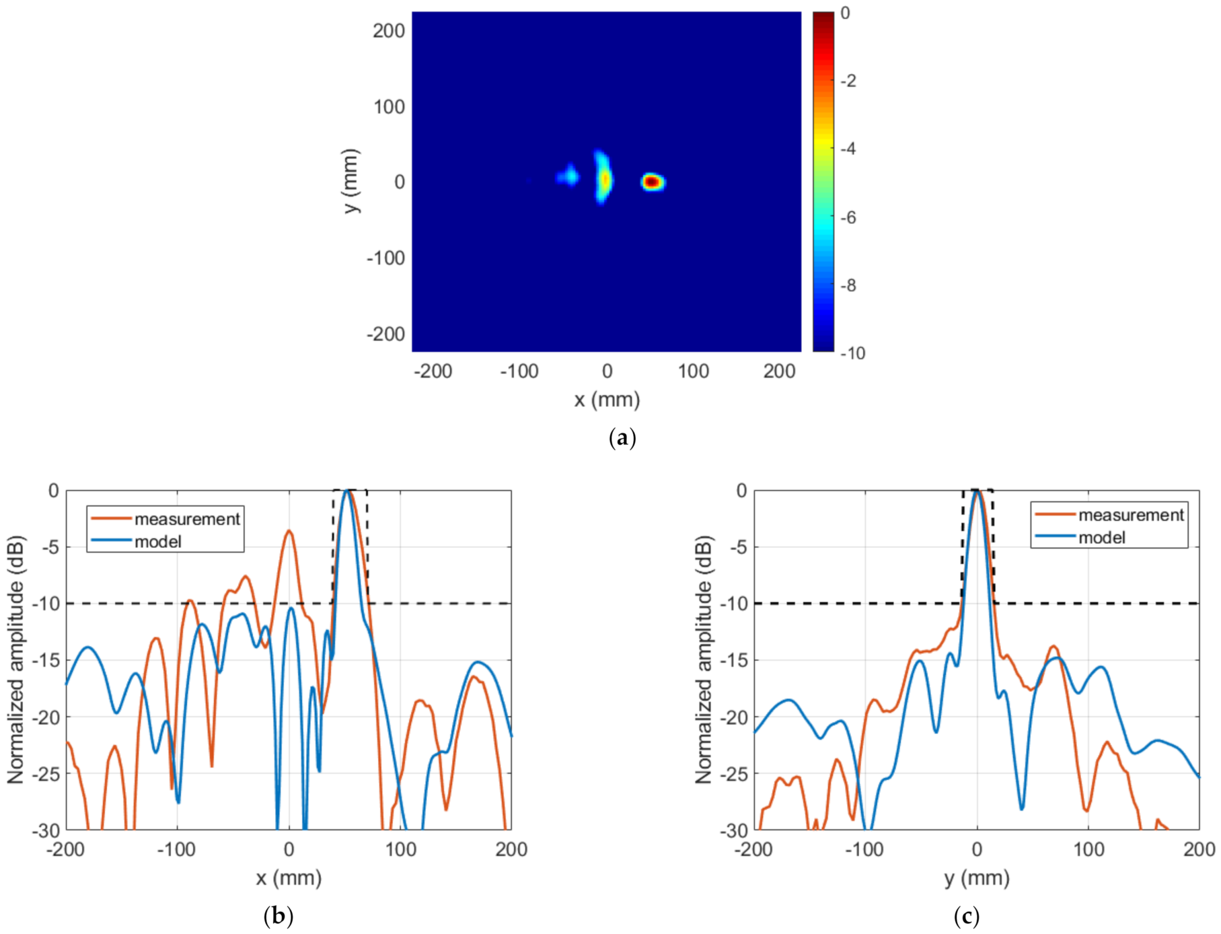
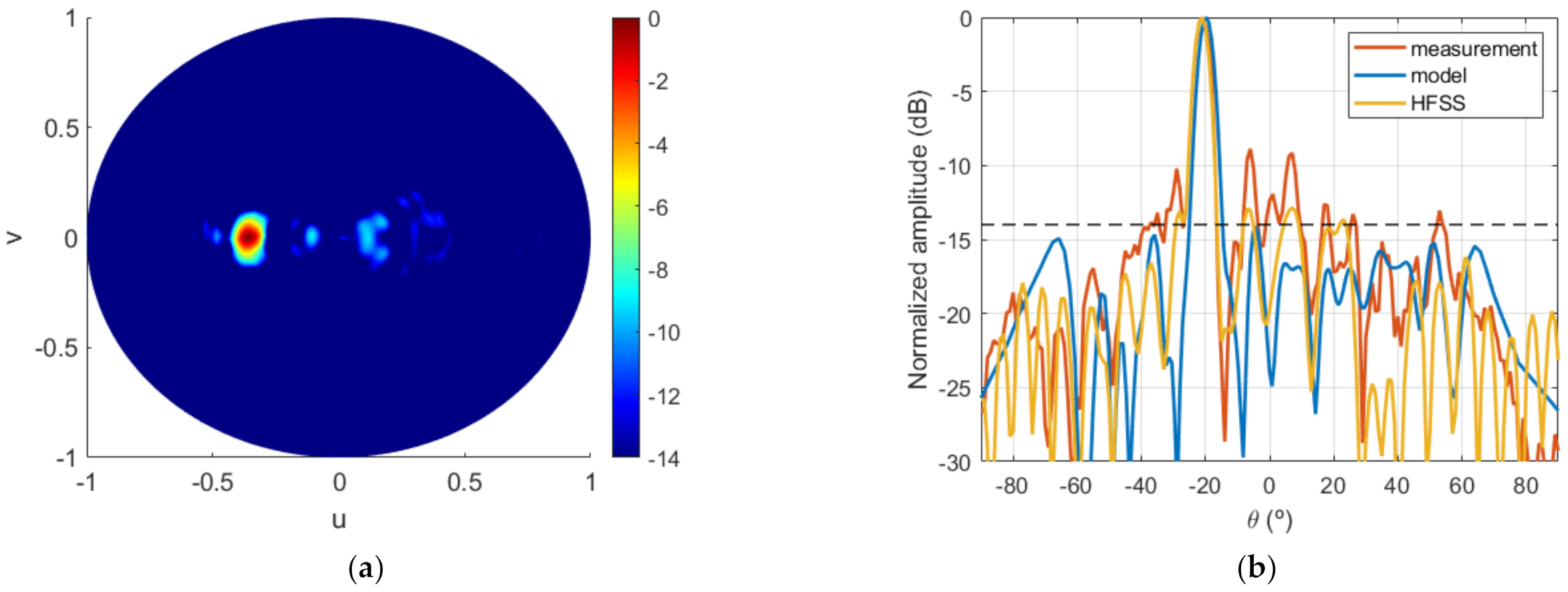
3.2. Case 2: Far-Field Beam and Near-Field Spot
- FF: pointing at with SLL lower than −14 dB outside the main lobe.
- NF: spot at the position with , spot width on the order of one wavelength, and level lower than −10 dB outside the spot.
4. Conclusions
Author Contributions
Funding
Institutional Review Board Statement
Informed Consent Statement
Data Availability Statement
Conflicts of Interest
References
- Osseiran, A.; Boccardi, F.; Braun, V.; Kusum, K.; Marsch, P.; Maternia, M.; Queseth, O.; Schellmann, M.; Schotten, H.; Taoka, H.; et al. Scenarios for 5G mobile and wireless communications: The vision of the METIS project. IEEE Commun. Mag. 2014, 52, 26–35. [Google Scholar] [CrossRef]
- Sakaguchi, K.; Haustein, T.; Barbarossa, S.; Strinati, E.C.; Clemente, A.; Destino, G.; Pärssinen, A.; Kim, I.; Chung, H.; Kim, J.; et al. Where, when, and how mmwave is used in 5G and beyond. IEICE Trans. Electron 2017, E100-C, 790–808. [Google Scholar] [CrossRef] [Green Version]
- Liu, S.L.; Lin, X.Q.; Zhu, Z.B. Ka-band multi-focus and pattern manipulation in near-field based on three-dimensional printed transmit-array antenna. IET Microw. Antennas Propag. 2020, 14, 500–514. [Google Scholar] [CrossRef]
- Vaquero, A.F.; Pino, M.R.; Arrebola, M.; Matos, S.A.; Costa, J.R.; Fernandez, C.A. Evaluation of a dielectric-only transmitarray for generating multi-focusing near-field spots using a cluster of feeds in the Ka-band. Sensors 2021, 21, 422. [Google Scholar] [CrossRef] [PubMed]
- Bucci, O.M.; Capozzoli, A.; D’Elia, G. Power pattern synthesis of reconfigurable conformal arrays with near-field constraints. IEEE Trans. Antennas Propag. 2004, 25, 132–141. [Google Scholar] [CrossRef]
- Butazzoni, G.; Vescovo, R. Power synthesis for reconfigurable arrays by phase-only control with simultaneous dynamic range ratio and near-field reduction. IEEE Trans. Antennas Propag. 2012, 60, 1161–1165. [Google Scholar] [CrossRef]
- Ayestarán, R.; León, G.; Pino, M.R.; Nepa, P. Wireless power transfer through simultaneous near-field focusing and far-field synthesis. IEEE Trans. Antennas Propag. 2019, 67, 5623–5633. [Google Scholar] [CrossRef]
- Ryan, C.G.M.; Chacharmir, M.R.; Shaker, J.; Bray, J.R.; Antar, Y.M.M.; Ittipiboon, A. A wideband transmitarray using dual-resonant double square rings. IEEE Trans. Antennas Propagat. 2010, 58, 1486–1493. [Google Scholar] [CrossRef]
- Phillion, R.H.; Okoniewski, M. Lenses for circular polarization using planar arrays of rotated passive elements. IEEE Trans. Antennas Propagat. 2011, 59, 1217–1227. [Google Scholar] [CrossRef]
- Clemente, A.; Dussopot, L.; Sauleau, R.; Potier, P.; Pouliguen, P. Wideband 400-element electronically reconfigurable transmitarray in X band. IEEE Trans. Antennas Propagat. 2013, 61, 5017–5027. [Google Scholar] [CrossRef]
- Massaccesi, A.; Pirinoli, P.; Bertana, V.; Scordo, G.; Marasso, S.L.; Cocuzza, M.; Dassano, G. 3D-Printable dielectric transmitarray with enhanced bandwidth at millimeter-waves. IEEE Access 2018, 6, 46407–46418. [Google Scholar] [CrossRef]
- Yi, X.J.; Su, T.; Wu, B.; Chen, J.Z.; Yang, L.; Li, X. A double-layer highly efficient and wideband transmitarray antenna. IEEE Access 2019, 7, 23285–23290. [Google Scholar] [CrossRef]
- Reis, J.R.; Vala, M.; Caldeirinha, R.F.S. Review paper on transmitarray antennas. IEEE Access 2019, 7, 94171–94188. [Google Scholar] [CrossRef]
- Hong, W.; Jiang, Z.H.; Yu, C.; Zhou, J.; Chen, P.; Yu, Z.; Zhang, H.; Yang, B.; Pang, X.; Jiang, M.; et al. Multibeam antenna technologies for 5G wireless communications. IEEE Trans. Antennas Propagat. 2017, 65, 6231–6249. [Google Scholar] [CrossRef]
- Quevedo-Teruel, O.; Ebrahimpouri, M.; Ghasemifard, F. Lens antennas for 5G communications Systems. IEEE Commun. Mag. 2018, 56, 36–41. [Google Scholar] [CrossRef]
- Orgeira, O.; León, G.; Fonseca, N.J.G.; Mongelos, P.; Quevedo-Teruel, O. Near-field focusing multibeam geodesic lens antenna for stable aggregate gain in far-field. IEEE Trans. Antennas Propagat. 2022, 70, 3320–3328. [Google Scholar] [CrossRef]
- Nayeri, P.; Liang, M.; Sabory-García, R.A.; Tuo, M.; Yang, F.; Gehm, M.; Xin, H.; Elsherbeni, A.Z. 3D printed dielectric reflectarrays: Low-cost high-gain antennas at sub-millimeter waves. IEEE Trans. Antennas Propagat. 2014, 62, 2000–2008. [Google Scholar] [CrossRef]
- Imbert, M.; Papió, A.; De-Flaviis, F.; Jofre, L.; Romeu, J. Design and performance evaluation of a dielectric flat lens antenna for millimeter-wave applications. IEEE Antennas Wirel. Propag. Lett. 2015, 14, 342–345. [Google Scholar] [CrossRef] [Green Version]
- Yi, H.; Qu, S.W.; Ng, K.B.; Chan, C.H.; Bai, X. 3-D printed millimeter-wave and terahertz lenses with fixed and frequency scanned beam. IEEE Trans. Antennas Propagat. 2016, 64, 442–449. [Google Scholar] [CrossRef]
- Vaquero, A.F.; Pino, M.R.; Arrebola, M.; Matos, S.A.; Costa, J.R.; Fernandez, C.A. Bessel beam generation using dielectric planar lenses at millimeter frequencies. IEEE Access 2020, 8, 216185–216196. [Google Scholar] [CrossRef]
- Loredo, S.; León, G. Synthesis algorithm for “quasi-planar” dielectric lenses. In Proceedings of the European Conference on Antennas and Propagation (EuCAP), Krakow, Poland, 31 March–5 April 2019. [Google Scholar]
- Loredo, S.; León, G.; Plaza, E.G. A fast approach to near-field synthesis of transmitarrays. IEEE Antennas Wirel. Propag. Lett. 2021, 20, 648–652. [Google Scholar] [CrossRef]
- Loredo, S.; León, G.; Robledo, O.F.; Plaza, E.G. Phase-only synthesis algorithm for transmitarrays and dielectric lenses. ACES J. 2018, 33, 259–264. [Google Scholar]
- Plaza, E.G.; León, G.; Loredo, S.; Las-Heras, F. A simple model for analyzing transmitarrays. IEEE Antennas Propag. Mag. 2015, 57, 131–144. [Google Scholar] [CrossRef]
- Buffi, A.; Nepa, P.; Manara, G. Design criteria for near-field-focused planar arrays. IEEE Antennas Propag. Mag. 2012, 54, 40–50. [Google Scholar] [CrossRef]
- Felicio, J.M.; Fernandes, C.A.; Costa, J.R. Complex permittivity and anisotropy measurement of 3D-printed PLA at microwave and millimeter waves. In Proceedings of the International Conference on Applied Electromagnetics and Communications, Dubrovnik, Croacia, 19–21 September 2016. [Google Scholar] [CrossRef]
- OpenSCAD. Available online: https://openscad.org/ (accessed on 26 April 2022).
- Ansys HFSS. Available online: https://www.ansys.com/products/electronics/ansys-hfss (accessed on 26 April 2022).


| Stage#1 | Stage#2 | Stage#3 | Dielectric TA | ||
|---|---|---|---|---|---|
| FF | % directions > −15 dB 1 | 0.0126% | 0.0211% | 0.0126% | 0.0169% |
| mean error (dB) | 0.07 | 0.91 | 0.50 | 0.57 | |
| variance (dB) | 0.00 | 0.25 | 0.04 | 0.11 | |
| NF | % positions >−10 dB 2 | -- | 0.3194% | 0.4956% | 0.4667% |
| mean error (dB) | -- | 0.57 | 0.33 | 0.64 | |
| variance (dB) | -- | 0.24 | 0.14 | 0.21 | |
| Number of iterations | 100 | 5 | 5 | -- | |
| Computing time | Workstation with Intel Core i7-9800X CPU @ 3.8 GHz | 450 ms | 70 s | 70 s | -- |
| Laptop with Intel Core i5-5200U CPU @ 2.2 GHz | 1.6 s | 3 min 30 s | 3 min 30 s | -- | |
| Stage#1 | Stage#2 | Stage#3 | Dielectric TA | ||
|---|---|---|---|---|---|
| FF | % directions > −15 dB 1 | 0.0000% | 3.4196% | 0.0970% | 0.0801% |
| mean error (dB) | -- | 1.21 | 0.13 | 0.23 | |
| variance (dB) | -- | 0.78 | 0.01 | 0.02 | |
| NF | % positions > −10 dB 2 | -- | 0.0123% | 0.1913% | 0.2044% |
| mean error (dB) | -- | 0.21 | 0.40 | 0.76 | |
| variance (dB) | -- | 0.01 | 0.11 | 0.39 | |
| Number of iterations | 100 | 5 | 5 | -- | |
| Computing time | Workstation with Intel Core i7-9800X CPU @ 3.8 GHz | 450 ms | 90 s | 90 s | -- |
| Laptop with Intel Core i5-5200U CPU @ 2.2 GHz | 1.6 s | 5 min 10 s | 5 min 10 s | -- | |
Publisher’s Note: MDPI stays neutral with regard to jurisdictional claims in published maps and institutional affiliations. |
© 2022 by the authors. Licensee MDPI, Basel, Switzerland. This article is an open access article distributed under the terms and conditions of the Creative Commons Attribution (CC BY) license (https://creativecommons.org/licenses/by/4.0/).
Share and Cite
Loredo, S.; Plaza, E.G.; León, G. Fast Transmitarray Synthesis with Far-Field and Near-Field Constraints. Sensors 2022, 22, 4355. https://doi.org/10.3390/s22124355
Loredo S, Plaza EG, León G. Fast Transmitarray Synthesis with Far-Field and Near-Field Constraints. Sensors. 2022; 22(12):4355. https://doi.org/10.3390/s22124355
Chicago/Turabian StyleLoredo, Susana, Enrique G. Plaza, and Germán León. 2022. "Fast Transmitarray Synthesis with Far-Field and Near-Field Constraints" Sensors 22, no. 12: 4355. https://doi.org/10.3390/s22124355