
Metaheuristic Algorithm-Based Vibration Response Model for a Gas Microturbine

 , , and
Abstract
:1. Introduction
2. Methods
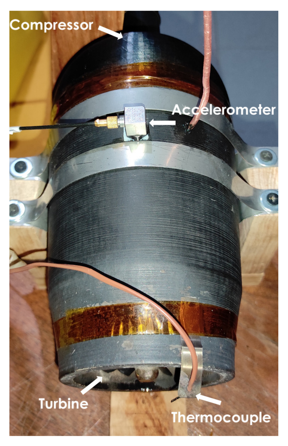
2.1. Experimental Setup
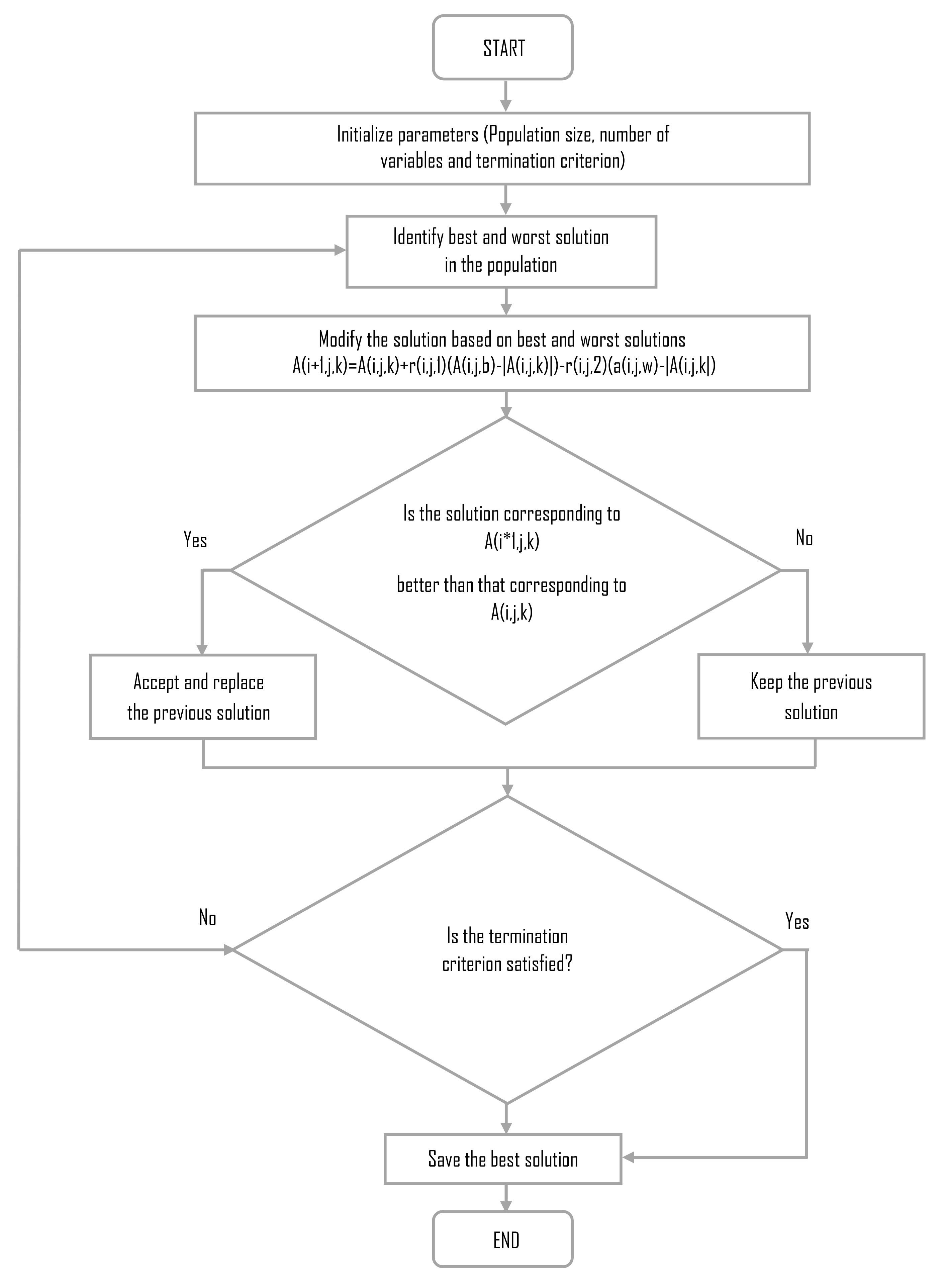
2.2. Response Surface Model Tuned by a Metaheuristic Algorithm
3. Results
4. Discussion
5. Conclusions
Author Contributions
Funding
Institutional Review Board Statement
Informed Consent Statement
Data Availability Statement
Acknowledgments
Conflicts of Interest
References
- Zhao, Q.; Yuan, J.; Jiang, H.; Yao, H.; Wen, B. Vibration control of a rotor system by shear thickening fluid dampers. J. Sound Vib. 2021, 494, 115883. [Google Scholar] [CrossRef]
- Zhao, Q.; Yuan, J.; Jiang, H.; Yao, H.; Wen, B. Basic research on machinery fault diagnostics: Past, present, and future trends. Front. Mech. Eng. 2018, 13, 264–291. [Google Scholar] [CrossRef] [Green Version]
- Tandon, N.; Parey, A. Condition Monitoring of Rotary Machines. In Condition Monitoring and Control for Intelligent Manufacturing; Springer: London, UK, 2006; pp. 109–136. [Google Scholar] [CrossRef]
- Kaminskiy, V.N.; Kaminskiy, R.V.; Lazarev, N.V.; Grigorov, I.N.; Kostyukov, A.V.; Korneev, S.A.; Kovaltsov, I.V.; Sergeev, A.S.; Gusak, A.A.; Sibiryakov, S.V. Development of test-benches for control and research tests of turbochargers. Izv. MGTU MAMI 2012, 1, 143–148. [Google Scholar] [CrossRef]
- Gomiciaga, R.; Keogh, P.S. Orbit Induced Journal Temperature Variation in Hydrodynamic Bearings. J. Tribol. 1999, 121, 77–84. [Google Scholar] [CrossRef]
- Zadorozhnaya, E.; Sibiryakov, S.; Hudyakov, V. Theoretical and Experimental Investigations of the Rotor Vibration Amplitude of the Turbocharger and Bearings Temperature. Tribol. Ind. 2017, 39, 452–459. [Google Scholar] [CrossRef] [Green Version]
- Zadorozhnaya, E.; Sibiryakov, S.; Lukovich, N. Calculated Estimates for the Thermal State and the Precession Amplitude of the Rotor in the Turbocharger Radial Bearing. Procedia Eng. 2017, 206, 716–724. [Google Scholar] [CrossRef]
- Gao, P.; Chen, Y.; Hou, L. Nonlinear thermal behaviors of the inter-shaft bearing in a dual-rotor system subjected to the dynamic load. Nonlinear Dyn. 2020, 101, 191–209. [Google Scholar] [CrossRef]
- Gu, L.; Chu, F. An analytical study of rotor dynamics coupled with thermal effect for a continuous rotor shaft. J. Sound Vib. 2014, 333, 4030–4050. [Google Scholar] [CrossRef]
- Ribeiro, P.; Manoach, E. The effect of temperature on the large amplitude vibrations of curved beams. J. Sound Vib. 2005, 285, 1093–1107. [Google Scholar] [CrossRef]
- Sun, W.; Yan, Z.; Tan, T.; Zhao, D.; Luo, X. Nonlinear characterization of the rotor-bearing system with the oil-film and unbalance forces considering the effect of the oil-film temperature. Nonlinear Dyn. 2018, 92, 1119–1145. [Google Scholar] [CrossRef]
- Sławiński, D.; Ziółkowski, P.; Badur, J. Thermal failure of a second rotor stage in heavy duty gas turbine. Eng. Fail. Anal. 2020, 115, 104672. [Google Scholar] [CrossRef]
- Gu, L. A Review of Morton Effect: From Theory to Industrial Practice. Tribol. Trans. 2018, 61, 381–391. [Google Scholar] [CrossRef]
- Tong, X.; Palazzolo, A.; Suh, J. Rotordynamic Morton Effect Simulation With Transient, Thermal Shaft Bow. J. Tribol. 2016, 138, 031705. [Google Scholar] [CrossRef]
- Plantegenet, T.; Arghir, M.; Jolly, P. Experimental analysis of the thermal unbalance effect of a flexible rotor supported by a flexure pivot tilting pad bearing. Mech. Syst. Signal Process. 2020, 145, 106953. [Google Scholar] [CrossRef]
- Nath, A.; Udmale, S.; Singh, S. Role of artificial intelligence in rotor fault diagnosis: A comprehensive review. Artif. Intell. Rev. 2021, 54, 2609–2668. [Google Scholar] [CrossRef]
- Mohamadi, M.R.; Abedini, M.; Rashidi, B. An adaptive multi-objective optimization method for optimum design of distribution networks. Eng. Optim. 2019, 52, 194–217. [Google Scholar] [CrossRef]
- Mishra, S.K.; Shakya, P.; Babureddy, V.; Ajay Vignesh, S. An approach to improve high-frequency resonance technique for bearing fault diagnosis. Measurement 2021, 178, 109318. [Google Scholar] [CrossRef]
- Çerçevik, A.E.; Özgür, A.; Hasançebi, O. Optimum design of seismic isolation systems using metaheuristic search methods. Soil Dyn. Earthq. Eng. 2020, 131, 106012. [Google Scholar] [CrossRef]
- Fiori de Castro, H.; Lucchesi Cavalca, K.; Ward Franco de Camargo, L.; Bachschmid, N. Identification of unbalance forces by metaheuristic search algorithms. Mech. Syst. Signal Process. 2010, 24, 1785–1798. [Google Scholar] [CrossRef]
- Abd Elaziz, M.; Elsheikh, A.H.; Oliva, D.; Abualigah, L.; Lu, S.; Ewees, A.A. Advanced Metaheuristic Techniques for Mechanical Design Problems: Review. Arch. Comput. Methods Eng. 2021, 29, 695–716. [Google Scholar] [CrossRef]
- Kumbhar, S.G.; Sudhagar P, E.; Desavale, R. Theoretical and experimental studies to predict vibration responses of defects in spherical roller bearings using dimension theory. Measurement 2020, 161, 107846. [Google Scholar] [CrossRef]
- Orosz, T.; Rassõlkin, A.; Kallaste, A.; Arsénio, P.; Pánek, D.; Kaska, J.; Karban, P. Robust Design Optimization and Emerging Technologies for Electrical Machines: Challenges and Open Problems. Appl. Sci. 2020, 10, 6653. [Google Scholar] [CrossRef]
- Rao, R. Jaya: A simple and new optimization algorithm for solving constrained and unconstrained optimization problems. Int. J. Ind. Eng. Comput. 2016, 7, 19–34. [Google Scholar] [CrossRef]
- Ostertagová, E. Modelling using Polynomial Regression. Procedia Eng. 2012, 48, 500–506. [Google Scholar] [CrossRef] [Green Version]
- Besharat, F.; Dehghan, A.A.; Faghih, A.R. Empirical models for estimating global solar radiation: A review and case study. Renew. Sustain. Energy Rev. 2013, 21, 798–821. [Google Scholar] [CrossRef]
- Rodríguez-Abreo, O.; Rodríguez-Reséndiz, J.; Montoya-Santiyanes, L.A.; Álvarez Alvarado, J.M. Non-Linear Regression Models with Vibration Amplitude Optimization Algorithms in a Microturbine. Sensors 2022, 22, 130. [Google Scholar] [CrossRef] [PubMed]
- Montoya-Santiyanes, L.A.; Domínguez-López, I.; Rodríguez, E.E. Análisis Experimental de la Frecuencia y Amplitud de Vibración en una Microturbina de Gas. Acad. J. 2021, 13, 282–286. [Google Scholar]
- Oliveira, M.V.M.; Cunha, B.Z.; Daniel, G.B. A model-based technique to identify lubrication condition of hydrodynamic bearings using the rotor vibrational response. Tribol. Int. 2021, 160, 107038. [Google Scholar] [CrossRef]
- Wang, N.; Jiang, D. Vibration response characteristics of a dual-rotor with unbalance-misalignment coupling faults: Theoretical analysis and experimental study. Mech. Mach. Theory 2018, 125, 207–219. [Google Scholar] [CrossRef]
- Sivasakthivel, P.S.; Velmurugan, V.; Sudhakaran, R. Prediction of vibration amplitude from machining parameters by response surface methodology in end milling. Int. J. Adv. Manuf. Technol. 2011, 53, 453–461. [Google Scholar] [CrossRef]
- Liu, C.; Jiang, D. Torsional vibration characteristics and experimental study of cracked rotor system with torsional oscillation. Eng. Fail. Anal. 2020, 116, 104737. [Google Scholar] [CrossRef]
- Yuvaraju, B.; Nanda, B. Prediction of vibration amplitude and surface roughness in boring operation by response surface methodology. Mater. Today Proc. 2018, 5, 6906–6915. [Google Scholar] [CrossRef]
- Prasad, B.S.; Babu, M.P. Correlation between vibration amplitude and tool wear in turning: Numerical and experimental analysis. Eng. Sci. Technol. Int. J. 2017, 20, 197–211. [Google Scholar] [CrossRef] [Green Version]
- Subramanian, M.; Sakthivel, M.; Sooryaprakash, K.; Sudhakaran, R. Optimization of end mill tool geometry parameters for Al7075-T6 machining operations based on vibration amplitude by response surface methodology. Measurement 2013, 46, 4005–4022. [Google Scholar] [CrossRef]
- Venkata Rao, K.; Murthy, P.B.G.S.N. Modeling and optimization of tool vibration and surface roughness in boring of steel using RSM, ANN and SVM. J. Intell. Manuf. 2018, 29, 1533–1543. [Google Scholar] [CrossRef]
- Alharbi, N. Experimental study on designing optimal vibration amplitude in ultrasonic assisted incremental forming of AA6061-T6. Eng. Sci. Technol. Int. J. 2022, 30, 101041. [Google Scholar] [CrossRef]


| Parameter | Description |
|---|---|
| Fuel | Butane/propane gas with maximum pressure of 3.5 kg/cm |
| Turbine blades outer/inner diameter | 68.6/40.5 mm |
| Compressor wheel outer/inner diameter | 64.5/32.8 mm |
| Turbine wheel diameter | 70 mm |
| Burner hole spacing | 10 mm |
| Number of gas outlet holes | 16 |
| Run | Temperature (C) | Standard Deviation | Frequency (Hz) | Standard Deviation | Amplitude (µm) | Standard Deviation |
|---|---|---|---|---|---|---|
| 1 | 151 | 17.8558 | 22.7 | 1.9465 | 3.4074 | 1.2252 |
| 2 | 291 | 5.0394 | 25.7 | 1.0593 | 2.3028 | 0.4475 |
| 3 | 145 | 0.4883 | 65.9 | 4.2804 | 4.8497 | 1.7376 |
| 4 | 302 | 2.5995 | 77.3 | 2.4517 | 4.2910 | 1.8773 |
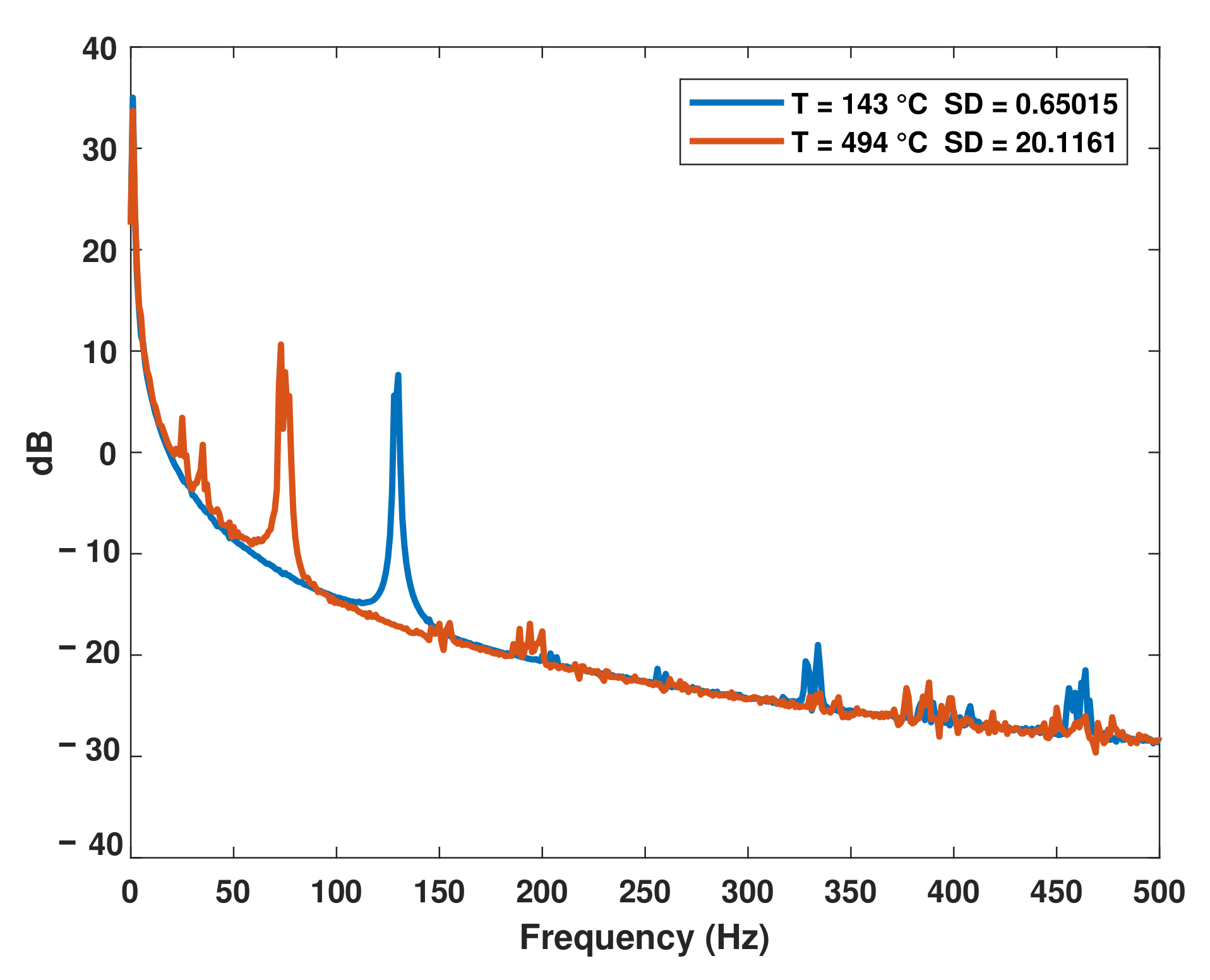
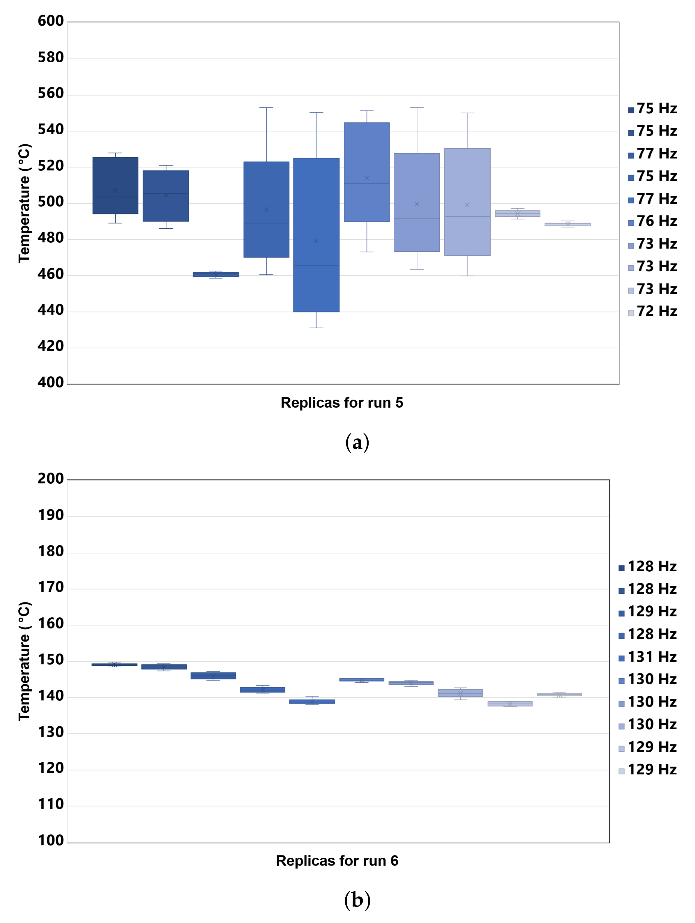
| 5 | 494 | 20.1161 | 74.6 | 1.7763 | 8.0382 | 2.1988 |
| 6 | 143 | 0.6501 | 129.2 | 1.0328 | 4.2209 | 0.6005 |
| 7 | 298 | 23.3357 | 118.4 | 6.3805 | 2.5392 | 1.2526 |
| 8 | 468 | 27.1826 | 127.2 | 6.4472 | 4.7098 | 1.1205 |
| Parameter | Value | Description |
|---|---|---|
| Population | 5000 | Number of vectors of proposed solutions |
| Variables | 12 | Length of coefficient vector |
| Maximum generations | 5000 | Maximum number of iterations |
| Low boundary | −1 | Lower limit of search |
| Up boundary | 1 | Upper limit of search |
| Order | Root of Average MSE (%) |
|---|---|
| 2 | 7.3524 |
| 3 | 4.7830 |
| 4 | 3.5040 |
| 5 | 3.4413 |
| 6 | 3.7629 |
| Coefficient | Value | Coefficient | Value |
|---|---|---|---|
| 1 | 1 | ||
| −1 | 1 | ||
| −0.6365 | −1 | ||
| −0.1521 | 0.6398 | ||
| 1 | −0.8662 | ||
| −0.7513 | 1 |
| Coefficient | Value | Coefficient | Value |
|---|---|---|---|
| 0.3677 | −0.6255 | ||
| −0.2627 | 1 | ||
| −0.3477 | 1 | ||
| −0.6472 | −0.0410 | ||
| 0.9872 | −1 | ||
| −0.6344 | 1 |
Publisher’s Note: MDPI stays neutral with regard to jurisdictional claims in published maps and institutional affiliations. |
© 2022 by the authors. Licensee MDPI, Basel, Switzerland. This article is an open access article distributed under the terms and conditions of the Creative Commons Attribution (CC BY) license (https://creativecommons.org/licenses/by/4.0/).
Share and Cite
Montoya-Santiyanes, L.A.; Rodríguez-Abreo, O.; Rodríguez, E.E.; Rodríguez-Reséndiz, J. Metaheuristic Algorithm-Based Vibration Response Model for a Gas Microturbine. Sensors 2022, 22, 4317. https://doi.org/10.3390/s22124317
Montoya-Santiyanes LA, Rodríguez-Abreo O, Rodríguez EE, Rodríguez-Reséndiz J. Metaheuristic Algorithm-Based Vibration Response Model for a Gas Microturbine. Sensors. 2022; 22(12):4317. https://doi.org/10.3390/s22124317
Chicago/Turabian StyleMontoya-Santiyanes, L. A., Omar Rodríguez-Abreo, Eloy E. Rodríguez, and Juvenal Rodríguez-Reséndiz. 2022. "Metaheuristic Algorithm-Based Vibration Response Model for a Gas Microturbine" Sensors 22, no. 12: 4317. https://doi.org/10.3390/s22124317