Article

Robust PMBM Filter with Unknown Detection Probability Based on Feature Estimation

1
Shanghai Institute of Technical Physics, Chinese Academy of Sciences, Shanghai 200083, China
2
Key Laboratory of Intelligent Infrared Perception, Chinese Academy of Sciences, Shanghai 200083, China
3
University of Chinese Academy of Sciences, Beijing 100049, China
*
Author to whom correspondence should be addressed.
Sensors 2022, 22(10), 3730; https://doi.org/10.3390/s22103730
Submission received: 9 April 2022 / Revised: 4 May 2022 / Accepted: 12 May 2022 / Published: 13 May 2022
(This article belongs to the Section Physical Sensors)

Abstract

:
This paper provides a solution for multi-target tracking with unknown detection probability. For the standard Poisson Multi-Bernoulli Mixture (PMBM) filter, the detection probability is generally considered a priori. However, affected by sensors, the features used for detection, and other environmental factors, the detection probability is time-varying and unknown in most multi-target tracking scenarios. Therefore, the standard PMBM filter is not feasible in practical scenarios. In order to overcome these practical restrictions, we improve the PMBM filter with unknown detection probability using the feature used for detection. Specifically, the feature is modeled as an inverse gamma distribution and the target kinematic state is modeled as a Gaussian distribution; the feature is integrated into the target kinematic state to iteratively estimate the target detection probability with the motion state. Our experimental results show that the proposed method outperforms the standard PMBM filter and the robust PMBM filter based on Beta distribution in the scenarios with unknown and time-varying detection probability. Further, we apply the proposed filter to a simulated infrared image to confirm the effectiveness and robustness of the filter.

1. Introduction

Multi-target tracking (MTT) refers to the process of jointly estimating the state and number of targets based on the observation data obtained by sensors [1]. MMT is a central problem both in military fields and civilian fields such as defense, surveillance, biomedical research, and autonomous driving [1,2,3,4,5]. Two main types of algorithms have been developed over the past few decades: traditional MTT algorithms and MTT algorithms based on random finite set (RFS) [6,7]. The former, which simplifies the MMT to single-target tracking by solving data association problem between targets and observations, mainly includes Multiple Hypotheses Tracking (MHT) [8,9], Joint Probabilistic Data Association (JPDA) [10], etc., while the latter, which has received much attention and extensive research, due to its providing an effective solution to the data association problem, mainly consists of a Probability Hypothesis Density (PHD) [11] filter, Cardinality-PHD (CPHD) [12] filter, Multi-target multi-Bernoulli (MeMBer) [6] filter, Generalized Labeled Multi-Bernoulli (GLMB) [13,14,15] filter, and Poisson Multi-Bernoulli Mixture (PMBM) [16] filter. Among these algorithms, the PMBM filter, which is a convolution of Poisson RFS and multi-Bernoulli mixture (MBM) RFS, is considered a promising tracking algorithm thanks to its high performance and reduced computational cost [2,17].
It is worth mentioning that the standard PMBM filter requires some a priori knowledge, such as the detection probability, and it is usually considered as a fixed value. However, the detection probability is unknown and even time-varying in practical applications; a significant mismatch in detection probability can result in a significant bias or erroneous estimation, which will affect the practicability of the algorithm. In order to make the filter more suitable for practical scenarios, the robust CPHD/PHD filter [18,19], robust multi-Bernoulli filter [20] and the Cardinality-Balance MeMBer filter [21], the GLMB filter with unknown detection probability [22], and the robust PMBM filter [23] have been successively proposed. All of them model the detection probability as a Beta distribution and iteratively estimate the variable with the targets’ state. However, the performance of these filters degrades when the detection probability is low; the performance also suffers when the model initialization parameters are poor.
Target detection probability depends on the sensor, environment and the features used for detection [24,25]. Generally, the signal-to-noise ratio (SNR) and the amplitude are the most widely used features for detection [26,27]. The SNR feature is introduced to PHD/CPHD to estimate the detection probability [25], while [26] introduces the amplitude to the PHD/CPHD filter to improve filters’ performance, and [28] introduces the amplitude to multi-sensor MeMBer/CPHD to estimate the detection probability; simulation results show that the performance of the filters is improved thanks to the above.
Inspired by [25,26,28], we improve the PMBM filter with unknown detection probability using the feature used for detection. Firstly, we model the feature as an inverse gamma distribution. Then, the feature is integrated into the target kinematic state which is modeled as a Gaussian distribution. In particular, the feature is independent with the kinematic state of targets due to the feature being a relatively stable variable which will not change significantly with the small change in target location. Finally, the detection probability and the motion state can be estimated iteratively. Two outcomes of the experiment can be summarized as (a) the tracking performance of the proposed filter is similar to the standard PMBM filter, where the detection probability is exactly known, fixed and high. Whereas in the low probability scenario, the Beta Gaussian Mixture (BGM-PMBM) filter and standard PMBM filter yield slightly higher error than the proposed filter, especially the BGM-PMBM filter. (b) when the detection probability is varying with time, the proposed filter can more accurately estimate the varying detection probability and has better performance. The results presented show the robustness and effectiveness of the proposed filter.
The key contribution of this paper is the derivation of a close-form solution to the robust PMBM filter recursion which can jointly estimate the target state and detection probability. The intent is to exploit the inverse gamma (IG) component to estimate the feature used for detection and thus the detection probability. The algorithm in this paper improves the tracking performance of the target under unknown detection probability, especially when the detection probability is relatively low.
The outline of the remainder of this paper is as follows. Section 2 introduces the necessary background knowledge of the proposed algorithm, including PMBM recursion and inverse gamma (IG) distribution. Section 3 derives the proposed filter and its implementation. Section 4 gives the simulation results with a linear multi-target filtering scenario. A conclusion is provided in Section 5.

2. Background

2.1. PMBM RFS Density

Let x k , 1 , , x k , N ( k ) and z k , 1 , , z k , M ( k ) denote the states of all N ( k ) targets and all M ( k ) measurements at time k , respectively. Then we have RFSs X k = { x k , 1 , , x k , N ( k ) } X , Z k = { z k , 1 , , z k , M ( k ) } Z which denote the multi-target state set and multi-target observation set, respectively. X denotes the state space and Z denotes the observation space.
According to the observation, the given non-empty state set X can be divided into two parts: undetected targets subsets X u and detected targets subsets X d . Hence the posterior density can be denoted as follows:
f ( X ) = X u X d = X f P ( X u ) f m b m ( X d ) ,
f P ( X u ) = e μ ( x ) d x x X u μ ( x ) ,
f m b m ( X d ) = j I i I j X i = X d i I j ω j , i f j , i ( X i ) ,
where f P ( X u ) is the Poisson density, denoting the undetected targets, μ ( x ) is the intensity function. f m b m ( X d ) is a multi-Bernoulli mixture denoting the potential targets which are detected at least once. ω j , i is the hypothesis weight and ω j , i = 1 , f j , i ( X i ) denotes the i th Bernoulli density in the j th global hypothesis, which is given by
f j , i ( X i ) = { 1 r j , i                     X i =   r j , i     p j , i ( x )             X i = { x }     0                                         o t h e r w i s e       ,
with r j , i denoting the existence probability and p j , i ( x ) denoting the single target density.

2.2. PMBM Filter

For the standard PMBM filter, the recursive processes are summarized as follows [16].
Prediction step: Suppose the intensity of Poisson RFS μ k 1 ( x ) and the MBM RFS { ω k 1 j , i , r k 1 j , i , p k 1 j , i ( x ) } k 1 j , i are given at time k 1 . The prediction step can be expressed by
(a) For Poisson Component
μ k | k 1 ( x ) = γ k ( x ) + f k | k 1 ( x | ζ ) P S , k ( ζ ) μ k 1 ( ζ ) d ζ
where γ k ( x ) is the intensity of the new born targets, μ k | k 1 ( x ) denotes the predicted intensity. f k | k 1 ( x | ζ ) and P S , k ( ζ ) are the transition density of state x given ζ and survival probability given ζ , respectively.
(b) For MBM Component
ω k | k 1 j , i = ω k 1 j , i
  r k | k 1 j , i = r k 1 j , i P S , k ( ζ ) p k 1 j , i ( ζ ) d ζ
p k | k 1 j , i ( x k ) f k | k 1 ( x | ζ ) P S , k ( ζ ) p k 1 j , i ( ζ ) d ζ
Update step: Given the predicted PMBM filter with parameters μ k | k 1 ( x ) and { ω k | k 1 j , i , r k | k 1 j , i , p k | k 1 j , i ( x , a ) } k 1 j , i at time k , the update step can be obtained based on the observations Z k .
(a) For Poisson Component
μ k | k ( x ) = ( 1 P D ) μ k | k 1 ( x )
where P D denotes the detection probability.
(b) For MBM Component: The update step of detected targets can be divided into two types.
Update for the targets detected for the first time:
r k P = e k ( z ) / ρ k P
p k P ( x | z ) = P D g k ( z | x ) μ k | k 1 ( x ) / e k ( z )
where
ρ k P = e k ( z ) + c ( z )
e k ( z ) = P D g k ( z | ζ ) μ k | k 1 ( ζ ) d ζ
where g k ( z | x ) is the likelihood function, and c ( z ) is the clutter intensity.
Update for the targets detected previously:
ω k j , i = { ω k | k 1 j , i × ( 1 r k | k 1 j , i + r k | k 1 j , i p k | k 1 j , i ( ζ ) ( 1 P D ) d ζ )     Z k = ω k | k 1 j , i r k | k 1 j , i × P D p k | k 1 j , i ( ζ ) g k ( z | ζ ) d ζ                                                             Z k
r k j , i = { r k | k 1 j , i p k | k 1 j , i ( ζ ) ( 1 P D ) d ζ 1 r k | k 1 j , i + r k | k 1 j , i p k | k 1 j , i ( ζ ) ( 1 P D ) d ζ                 Z k =                                                 1                                                                     Z k
p k j , i ( x | z ) = { ( 1 P D ) p k | k 1 j , i ( x ) p k | k 1 j , i ( ζ ) ( 1 P D ) d ζ   Z k =     P D g k ( z | x ) p k | k 1 j , i ( x ) P D p k | k 1 j , i ( ζ ) g k ( z | ζ ) d ζ Z k
After the update, we get all possible new single-target hypotheses, we have to go through all possible data association hypotheses to construct the global hypotheses. In order to reduce the cost, a Gibbs sampler [29] or Murty’s [14,16] algorithm can be employed to prune the number of the hypotheses to improve the computation efficiency. In this work, we use the Gibbs sampler due to the lower computation complexity [30]. The detail implementation can be found in [29,31].

2.3. Gamma Distribution and Inverse Gamma Distribution

The probability density of the inverse Gamma distribution for non-negative variable a can be denoted as [25]
I G ( a ; s ; t ) = t s Γ ( s ) a s 1 exp ( t a ) ,
where shape parameter s > 0 and scale parameter t > 0 . Γ ( s ) is Gamma function. The mode at which the probability density function is the maximum is t / ( s + 1 ) . The mean value and variance of the IG distribution is t / ( s 1 ) and t 2 / [ ( s 1 ) 2 ( s 2 ) ] respectively.
The probability density of the Gamma distribution for variable a is as follows
G ( a ; s ; t ) = t s Γ ( s ) a s 1 exp ( t a )
where shape parameter s > 0 and scale parameter t > 0 . The mode and the mean value are ( s 1 ) / t and s / t respectively.

3. The Proposed Robust Filter with Unknown Detection Probability

In this section, the specific implementation of the robust PMBM filter based on inverse gamma Gaussian mixture (IGGM) distribution is introduced.

3.1. Target State Model and Observation Model

Similar to [23,25], the feature denoted by a is augmented to x which denotes the kinematic state of a single target and consists of positions and velocities; let x ^ expresses the new state of a single target, i.e., x ^ = ( x , a ) . The variable a denotes the SNR throughout in this paper. The detection probability and survival probability at time k can be expressed as
P D , k ( x ^ ) = P D , k ( a ) ,
P s , k ( x ^ ) = P s , k ( x )
The kinematic state and the feature are modeled as Gaussian distribution and inverse gamma distribution, respectively, so the target density at time k can be denoted by the IGGM as
f k ( x , a ) = i = 1 J k ω k i N ( x ; m k i ; P k i ) I G ( a ; s k i ; t k i )
where J k is the number of the IGGM components at time k , and ω k i is the weight of the i th IGGM component. m and P are the mean and covariance of Gaussian density. The Markov transition density can be expressed as
f k | k 1 ( x ^ | ζ ^ ) = f k | k 1 ( x , a | ζ , α ) = f k | k 1 ( x | ζ ) f k | k 1 ( a | α ) ,
f k | k 1 ( x | ζ ) = N ( x ; F k 1 x k 1 ; Q k 1 ) ,
f k | k 1 ( a | α ) = I G ( a ; s k | k 1 ; t k | k 1 ) ,
s k | k 1 = k s s k 1 , 0 < k s < 1 ,
t k | k 1 = t k 1 s k 1 1 ( k s s k 1 1 ) ,
F k 1 and Q k 1 denote the state transition matrix and process noise covariance.
Similarly, the observation state is also augmented; the new observation state is expressed as z ^ = ( z , h ) where z and h are the observation of position and the feature, respectively. The likelihood function of the augmented state at time k can be expressed
g k ( z ^ | x ^ ) = g k ( z , h | x , a ) = g k ( z | x ) g k ( h | a ) = N ( z ; H k x ; R k ) G ( h ; ξ ; ξ a ) ,
H k and R k represent the observation matrix and observation noise covariance, respectively. The likelihood of feature is gamma distribution which ensures the conjugation of the PMBM filter.
The update of the IG component can be calculated as follows [25].
I G ( a ; s k | k 1 ; t k | k 1 ) g k ( h | a ) = t k | k 1 s k | k 1 Γ ( s k | k 1 ) a s k | k 1 1 exp ( t k | k 1 a ) × G ( h ; ξ k ; ξ k a ) = A · I G ( a ; s k ; t k )
A = t k | k 1 s k | k 1 Γ ( s k | k 1 ) ξ ξ Γ ( ξ ) Γ ( s k ) t k s k h ξ 1
s k = s k | k 1 + ξ
t k = t k | k 1 + h ξ

3.2. The Implementtation of Proposed Algorithm

Similar to the standard PMBM filter, the proposed algorithm can be divided into Poisson components and MBM components which denote undetected targets and potentially detected targets, respectively. Besides, the iterative recursion of the Gaussian component is similar to Kalman filter (KF).
Prediction step: Given the intensity of Poisson RFS μ k 1 ( x , a ) and MBM RFS { ω k 1 j , i , r k 1 j , i , p k 1 j , i ( x , a ) } k 1 j , i at time k 1 . The prediction step can be expressed by
(a) For Poisson Component
μ k | k 1 ( x , a ) = γ k ( x k , a k ) + i = 1 J k 1 u ω k | k 1 i , u N ( x ; m k | k 1 i , u ; P k | k 1 i , u ) I G ( a ; s k | k 1 i , u ; t k | k 1 i , u )
where s k | k 1 i , u and t k | k 1 i , u can be obtained according to (25), (26). γ k ( x k , a k ) is also the IGGM form.
ω k | k 1 i , u = p S , k ω k 1 i , u ,
m k | k 1 i , u = F k 1 m k 1 i , u ,
P k | k 1 i , u = Q k 1 + F k 1 P k 1 i , u F k 1 T .
(b) For MBM Component
ω k | k 1 j , i = ω k 1 j , i ,
r k | k 1 j , i = p S , k r k 1 j , i ,
p k | k 1 j , i ( x , a ) = N ( x ; m k | k 1 j , i ; P k | k 1 j , i ) I G ( a ; s k | k 1 j , i ; t k | k 1 j , i ) ,
where
m k | k 1 j , i = F k 1 m k 1 j , i ,
P k | k 1 j , i = Q k 1 + F k 1 P k 1 j , i F k 1 T ,
s k | k 1 i , u and t k | k 1 i , u can be obtained according to (25) and (26).
Update step: Suppose the predicted intensity of Poisson RFS μ k | k 1 ( x , a ) and MBM RFS { ω k | k 1 j , i , r k | k 1 j , i , p k | k 1 j , i ( x , a ) } k 1 j , i are given at time k , the update step can be expressed by
(a) For Poisson Component
μ k ( x , a ) = ( 1 P D , k ( a k | k 1 i , u ) ) μ k | k 1 ( x , a ) .
(b) For MBM Component: The update step of detected targets can be divided into two types
Update for the targets detected for the first time
r k P = e k ( z , h ) / ρ k P ( z , h ) ,
p k P ( x , a | z , h ) = 1 e k ( z , h ) × i = 1 J k | k 1 u P D , k ( a k | k 1 i , u ) ω k , 2 i , u A k , 2 ( h ) q k , 2 ( z ) × N ( x ; m k , 2 i , u ; P k , 2 i , u ) I G ( a ; s k , 2 i , u ; t k , 2 i , u )
where J k | k 1 u = J k 1 u + | γ k | ,   ω k , 2 i , u = ω k | k 1 i , u , s k , 2 i , u = s k | k 1 i , u + ξ , t k , 2 i , u = t k | k 1 i , u + ξ h .
ρ k P ( z , h ) = e k ( z , h ) + κ k ( z , h ) ,
κ k ( z , h ) = λ k c ( z ) I G ( a ; s k , 2 κ ; t k , 2 κ ) g ( h | a ) = λ k c ( z ) ( t k , 2 κ ) s k , 2 κ Γ ( s k , 2 κ ) ξ ξ Γ ( ξ ) Γ ( s k , 2 κ + ξ ) ( t k , 2 κ + h ξ ) ( s k , 2 κ + ξ ) h ξ 1 ,
e k ( z , h ) = l = 1 J k | k 1 u P D , k ( a k | k 1 l , u ) ω k | k 1 l , u q k , 2 ( z ) A k , 2 ( h ) ,
A k , 2 ( h ) = ( t k | k 1 i , u ) s k | k 1 i , u Γ ( s k | k 1 i , u ) ξ ξ Γ ( ξ ) Γ ( s k | k 1 i , u + ξ ) ( t k | k 1 i , u + h ξ ) ( s k | k 1 i , u + ξ ) h ξ 1 ,
q k , 2 ( z ) = N ( z ; H k m k | k 1 i , u ; H k P k | k 1 i , u H k T + R k ) ,
m k , 2 i , u = m k | k 1 i , u + K ( z H k m k | k 1 i , u ) ,
P k , 2 i , u = ( I K H k P k | k 1 i , u ) ,
K = P k | k 1 i , u H k T ( H k P k | k 1 i , u H k T + R k ) 1 ,
where κ k ( z , h ) is the clutter intensity.
Update for the targets detected previously
ω = { ω k | k 1 j , i × ( 1 r k | k 1 j , i + r k | k 1 j , i ( 1 P D , k ( a k | k 1 j , i ) )   Z k = ω k | k 1 j , i r k | k 1 j , i P D , k ( a k | k 1 j , i ) q k , 4 ( z ) A k , 4 ( h )                                 Z k ,
r = { r k | k 1 j , i ( 1 P D , k ( a k | k 1 j , i ) ) 1 r k | k 1 j , i + r k | k 1 j , i ( 1 P D , k ( a k | k 1 j , i ) )                 Z k =                                       1                                                                   Z k
p = { N ( x ; m k , 3 j , i ; P k , 3 j , i ) I G ( a ; s k , 3 j , i ; t k , 3 j , i )       Z k =     N ( x ; m k , 4 j , i ; P k , 4 j , i ) I G ( a ; s k , 4 j , i ; t k , 4 j , i )       Z k ,
where m k , 3 j , i = m k | k 1 j , i , P k , 3 j , i = P k | k 1 j , i , s k , 3 j , i = s k | k 1 j , i , t k , 3 j , i = t k | k 1 j , i , s k , 4 j , i = s k | k 1 j , i + ξ , t k , 4 j , i = t k | k 1 j , i + ξ h .
q k , 4 ( z ) = N ( z ; H k m k | k 1 j , i ; H k P k | k 1 j , i H k T + R k ) ,
A k , 4 ( h ) = ( t k | k 1 j , i ) s k | k 1 j , i Γ ( s k | k 1 j , i ) ξ ξ Γ ( ξ ) Γ ( s k | k 1 j , i + ξ ) ( t k | k 1 j , i + h ξ ) ( s k | k 1 j , i + ξ ) h ξ 1 ,
m k , 4 j , i = m k | k 1 j , i + K ( z H k m k | k 1 j , i ) ,
P k , 4 j , i = ( I K H k P k | k 1 j , i ) ,
K = P k | k 1 j , i H k T ( H k P k | k 1 j , i H k T + R k ) 1 .
The feature can be extracted by
a k | k 1 j , i = t k | k 1 j , i s k | k 1 j , i 1 .
Then, the detection probability can be obtained by
P D , k ( a ) = { ε 1 · ( exp ( a S N R t h δ 1 ) ε 2 )                         a < S N R t h   ε 1 · ( 2 exp ( a S N R t h δ 2 ) ε 2 )     a S N R t h  
Algorithm 1 gives the pseudo-code of the proposed algorithm.
Algorithm 1 Description of the proposed robust filter
Input:   μ k 1 ( x ^ ) ,   { ω k 1 j , i , r k 1 j , i , p k 1 j , i ( x ^ ) } k 1 j , i ,   γ k ( x ^ ) ,   z ^ k
Output:   μ k ( x ^ ) ,   { ω k j , i , r k j , i , p k j , i ( x ^ ) } k j , i ,   P D , k   and   estimated   object   states
Prediction process:
  Poisson process: see Formula (32)
  MBM process:
   for jth global hypothesis do
        for ith Bernoulli in the jth global hypothesis do
     see Formulas (36)–(38)
        end for
   end for
Update process:
  Poisson process: see Formula (41)
  MBM process:
       If the target is the first detected
     for each measurement do
      Formulas (42) and (43)
     end for
   If the target detected before
          for ith Bernoulli in the jth global hypothesis do
             Formulas (52)–(54)
     end for
Construct global hypothesis: Gibbs sampler
Estimate target state and detection probability
Pruning and Merging

3.3. The Computation Complexity of the Proposed Algorithm

Before discussing the computation complexity of the proposed algorithm (IGGM-PMBM), we first analyze the computation complexity of Gaussian Mixture-PMBM (GM-PMBM) [32].
Suppose that the number of association hypotheses is | A k 1 | k 1 | after the prediction step at time k 1 , it takes N k | k 1 u m k + | A k 1 | k 1 | N k | k 1 m k + | A k 1 | k 1 | ( m k / N k | k 1 ) N k | k 1 steps to calculate the updated PMBM density at time k , where N k | k 1 u , N k | k 1 and m k are the number of the unknown target components, the MB’s components, and the measurements after the prediction step, respectively. Thus, the complexity of the GM-PMBM update is O ( N k | k 1 u m k + | A k 1 | k 1 | ( m k / N k | k 1 ) N k | k 1 ) . The detailed calculations can be found in [33]. From the results, it can be seen that the computation complexity of the PMBM filter is related to the number of the unknown target components, the MB’s components, and the measurements. The framework of IGGM-PMBM filter is unchanged relative to the GM-PMBM filter. Thus, the complexity of the IGGM-PMBM filter does not increase relative to the GM-PMBM filter in theory. However, due to the need to propagate an additional function, i.e., inverse gamma distribution, the IGGM-PMBM filter has a slightly higher complexity compared to the GM-PMBM filter. The same analysis applies to BGM-PMBM filter. Besides, this IGGM-PMBM filter does not increase the complexity of the BGM-PMBM filter but improves the performance.

4. Simulation Setup and Results

4.1. Simulation Scenario 1

As a verification for the proposed algorithm, the simulation data in [16] was selected. The area is [110, 180] m × [110, 180] m. There are four targets; Figure 1 is the targets’ real track. The targets are all born at Step 1 and alive all the time, except the blue one which dies at Step 40. Targets kinematic state include the position and velocity x = ( p x ; v x ; p y ; v y ) and each observation is a vector of position z = ( z x ; z y ) . The parameters used in (23) and (27) are given as
F = I 2 ( 1       T 0       1 ) , Q = q I 2 ( T 3 / 3       T 2 / 2 T 2 / 2           T       ) H = I 2 ( 1 0 ) , R = I 2
where is the Kronecker product, T = 1 is the sampling period, and q = 0.01 . In formula (25), which denotes the prediction step of IG distribution, k s is set as 0.9. The parameter ξ in likelihood function g k ( h | a ) for feature d is 10. In formula (61), we set δ 1 = 4 , δ 2 = 2 , and ε 1 = ( 2 exp ( S N R t h / δ 1 ) ) 1 , ε 2 = exp ( S N R t h / δ 1 ) . In the simulation, we let the survival probability be 0.99, i.e., p S , k = 0.99 . The parameters used in the pruning and merging processes are the same as in [16,25]. The proposed algorithm was compared with the GM-PMBM filter and the BGM-PMBM filter which can also estimate the detection probability online. The generalized optimal sub-pattern (GOSPA) [34] assignment metric with parameters α = 2 is employed to assess the performance of filters. The GOSPA is defined as
d p ( c , 2 ) ( X , Y ) [ min γ Γ ( | X | , | Y | ) ( ( i , j ) γ d ( x i , y i ) p + c p 2 ( | X | + | Y | 2 | γ | ) ) ] 1 P
The Γ ( | X | , | Y | ) denotes the assignment set between { 1 , 2 , | X | } and { 1 , 2 , | Y | } . In this situation, c l 2 ( · , · ) = ( i , j ) γ d ( x i , y j ) p , c m 2 ( · , · ) = c p ( | X | | γ | ) 2 and c f 2 ( · , · ) = c p ( | Y | | γ | ) 2 denote the location error (LE), miss error (ME), and false error (FE), respectively. Besides c = 1 , p = 2 .
There are two cases to be considered: fixed detection probability and time-varying probability.
Case 1-Fixed detection probability: In this scenario, the target detection probability is fixed. Targets are born according to a Poisson process with intensity:
γ k ( x k , a k ) = i = 1 4 ω γ N ( x ; m γ i ; P γ i ) I G ( a ; s γ i ; t γ i )
where ω γ = 0.03 and Gaussian density with mean [100;0;100;0], covariance d i a g ( [ 150 2 , 1 , 150 2 , 1 ] ) . s γ i = 51 and t γ i = 500 denotes the parameters of IG distribution [25], thus the feature used for detection is 10. Clutter is also a Poisson process with intensity κ k ( z , h ) = λ κ I G ( a ; s k κ ; t k κ ) g ( h | a ) , where the clutter rate is   λ κ = 10 . The parameters of IG distribution are s k κ = 31 and t k κ = 280 . The parameters are summarized in Table 1. The parameters used in the BGM distribution are the same as in [23].
In this simulation, we set the S N R t h as two different values: 9 and 5.5, thus the corresponding detection probability is 0.68 and 0.94 respectively.
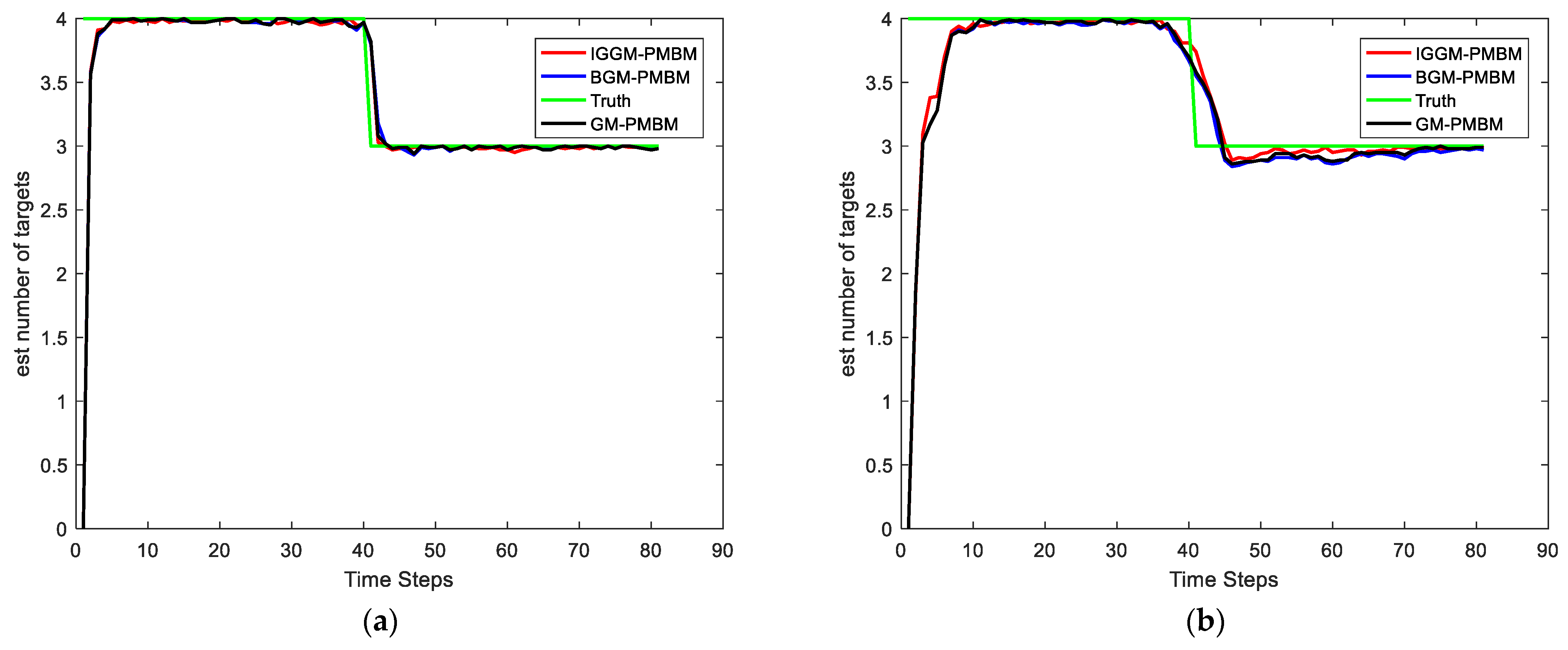
 Figure 2 and Figure 3 show the average results, corresponding to the performance metrics on their GOSPA error and the number of targets. In 
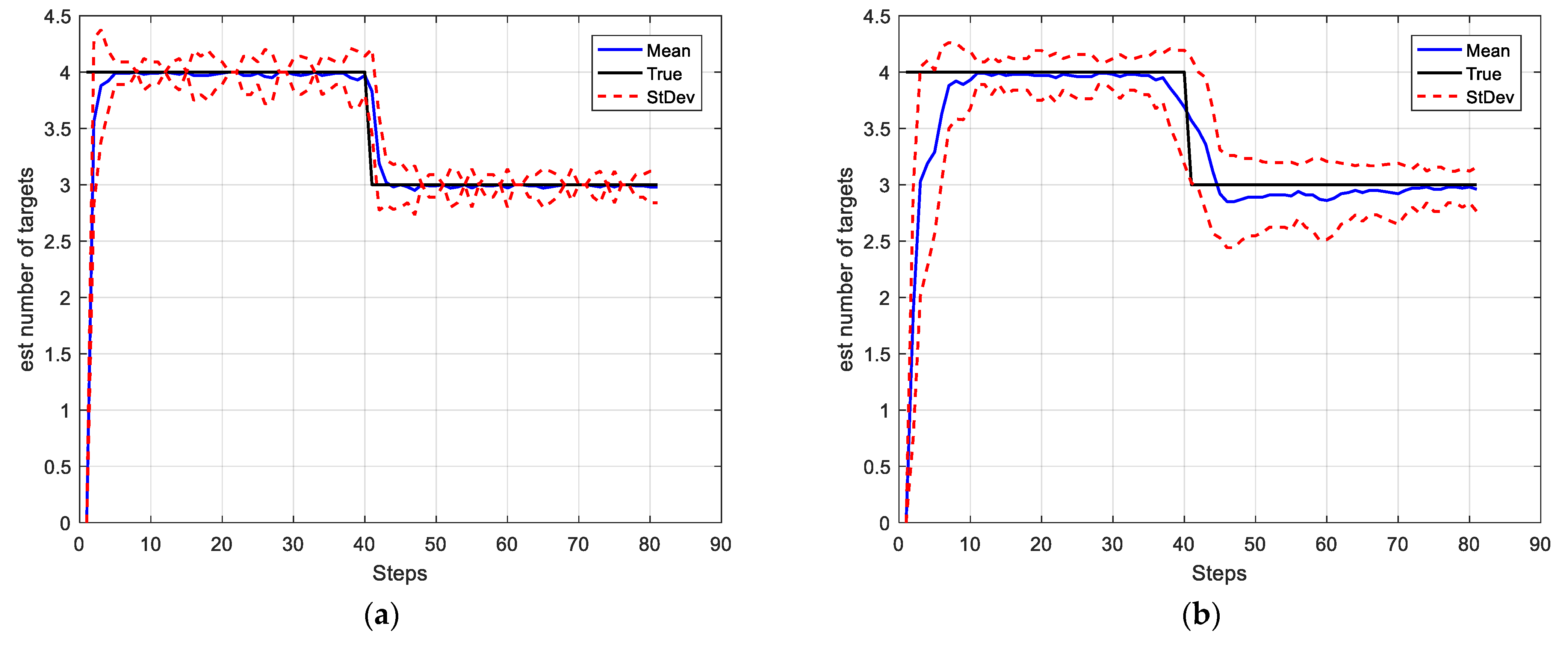
Figure 2, the result shows that the multitarget tracking performance of the proposed IGGM-PMBM filter is similar to the standard GM-PMBM filter with the similar GOSPA distance, where the detection probability is exactly known, fixed and high. Whereas in the low probability scenario, the BGM-PMBM filter and GM-PMBM filter yield slightly higher GOSPA error than IGGM-PMBM, especially the BGM-PMBM. This simulation shows that the proposed IGGM-PMBM filter outperforms the BMG-PMBM filter and GM-PMBM filter with low detection probability. The standard deviation range (StDev) values of estimated number of targets of IGGM-PMBM and BGM-PMBM are shown in Figure 4 and 
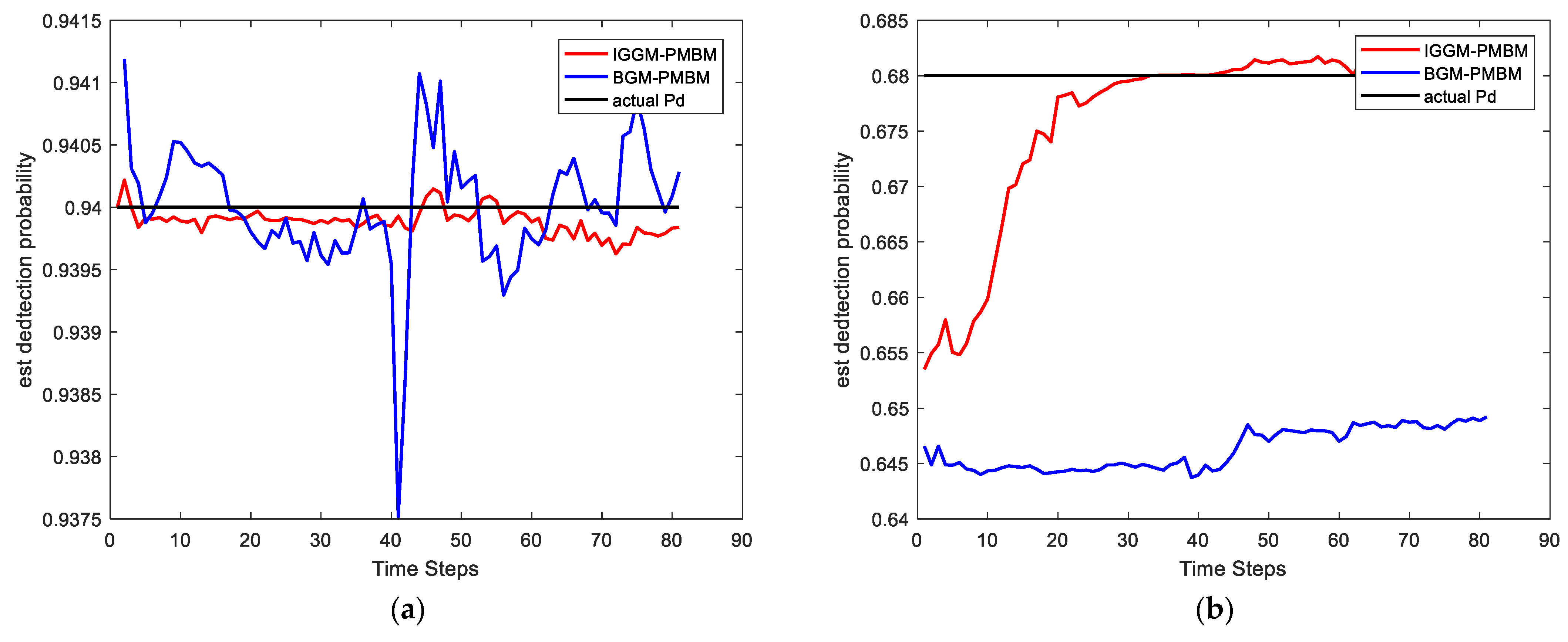
Figure 5. On the other hand, it can be seen in Figure 6 that the estimation of P D of IGGM-PMBM is more accurate. 
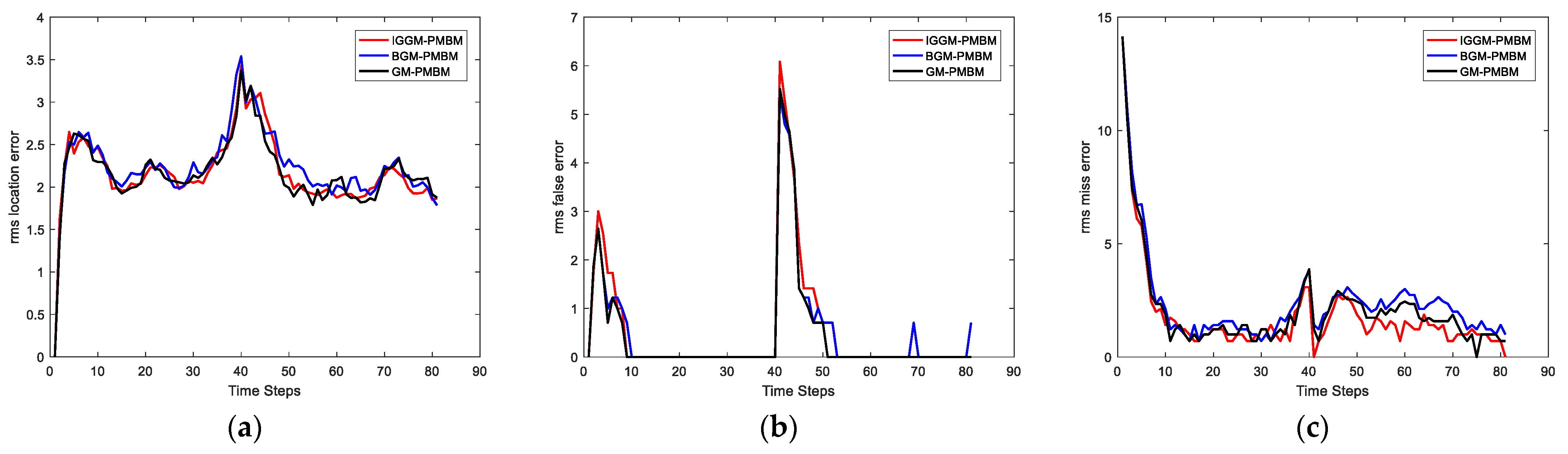
Figure 7 gives the comparisons of LE, ME, and FE when the detection probability is 0.68. The performance comparisons in terms of average GOSPA, LE, ME, and FE with different parameters (detection probabilities and clutter rates) are shown in Table 2. The results show that the performance of the proposed IGGM-PMBM filter is better than the BGM-PMBM filter and the GM-PMBM filter under the same parameters.
The three filters are run separately on an AMD Core 3.20 GHz CPU PC with 16 GB RAM and MATLAB R2021b. The complexity is also illustrated by comparing the computational time. Based on 100 Monte Carlo runs, the average computational times of the three filters are shown in Table 3. It can be seen that the computation complexity of IGGM-PMBM is slightly higher than the GM-PMBM filter in a high detection probability scenario, and with the detection probability decreasing, the IGGM-PMBM filter costs more time to tackle the unknown target detection probability situation. Besides, the IGGM-PMBM filter has almost the same complexity as the BGM-PMBM filter.
Case 2-Changing detection probability: In this scenario, the detection probability is varying with time. We set different parameters to express the different feature values for detection as Table 4. The S N R t h in this case is 5.5, thus the detection probabilities are 0.94, 0.81, and 0.69 respectively. Other parameters are the same as in Case 1. The average GOSPA error, LE, FE, ME, and cardinality estimate as well as estimate of P D are shown in Figure 8. It can be seen that the estimates of P D of the IGGM-PMBM filter is more accurate than BGM-PMBM filter for each segment. Moreover, the GOSPA errors of the proposed IGGM-PMBM is smaller than that of BGM-PMBM. Figure 9 gives the StDev of the estimated number of targets of the IGGM-PMBM filter and BGM-PMBM filter under the detection probability vary.

4.2. Simulation Scenario 2

We simulate a long wave infrared image of the movement of space targets using Satellite Tool Kit (STK). The image is 1024 × 1024 pixels, and there are 5400 frames. Figure 10 is the real trajectory of each target in the infrared image. We only track the centroid of the target in this experiment. There are a total of 9 targets, of which target 1 is always in the center of the image. Figure 11 shows the birth state of each target. As shown in Table 5, the birth state of each target including the position and velocity is set according to the target initial states. The covariance is d i a g ( [ 1 , 1 , 1 , 1 ] ) .The initial value of the feature for each target is different, and the parameters s γ and t γ of IG distribution are different at the birth time. The number of frames in which the target is born and the number of frames in which it dies are also given in Table 5. In this scenario, S N R t h is 5.5. Other parameters are the same as in simulation scenario1.
Figure 12 gives the performance of the IGGM-PMBM filter used in the infrared image. Obviously, the filter is effective for the infrared image.

5. Conclusions

In order to solve the problem of unknown detection probability and improve the accuracy when the low detection probability is low, we propose a novel PMBM filter based on the feature estimation for multi-target tracking. We model the feature as an inverse gamma distribution and integrate it into the kinematic state of targets. The feature can be estimated along with the motion state of the target, so as to further calculate the detection probability. The feature is related to detection and can be actually measured which can improve the accuracy of the detection probability estimation. The simulation results also show that the proposed algorithm can accurately estimate the detection probability and outperforms the GM-PMBM filter and BGM-PMBM filter with slightly lower GOSPA error especially when the detection probability is low. The proposed algorithm was then used in an infrared simulation scenario, which demonstrated the robustness and the effectiveness of the proposed algorithm. With the increase in space targets and development of autonomous driving and other fields, more and more radar data and space-based infrared image data will be obtained. Thus, the verification of the proposed algorithm using real data such as radar data and infrared images data would be a worthwhile subject of future study. Extending the proposed algorithm with unknown information is also a topic worthy of study.

Author Contributions

Y.W. performed the simulation and wrote the paper; X.C. simulated the infrared image and offered some useful suggestions with regard to methodology with P.R. All authors have read and agreed to the published version of the manuscript.

Funding

This research was funded by National Natural Science Foundation of China, grant number 62175251.

Institutional Review Board Statement

Not applicable.

Informed Consent Statement

Not applicable.

Data Availability Statement

Not applicable.

Conflicts of Interest

The authors declare no conflict of interest.

References

  1. Vo, B.-N.; Mallick, M.; Bar-Shalom, Y.; Coraluppi, S.; Osborne, R.; Mahler, R.; Vo, B.-T. Multitarget tracking. Wiley Encycl. Electr. Electron. Eng. 2015, 2015. [Google Scholar]
  2. Bohnsack, E.; Lilja, A. Multi-Object Tracking Using Either End-to-End Deep Learning or PMBM Filtering. Master’s Thesis, Chalmers University Oftechnology, Gothenburg, Sweden, 2019. [Google Scholar]
  3. Bouraya, S., Jr.; Belangour, A. Multi object tracking: A survey. In Proceedings of the Thirteenth International Conference on Digital Image Processing (ICDIP 2021), Singapore, 20–23 May 2021; International Society for Optics and Photonics: Bellingham, DC, USA, 2021; p. 118780. [Google Scholar]
  4. Pang, S.; Radha, H. Multi-Object Tracking using Poisson Multi-Bernoulli Mixture Filtering for Autonomous Vehicles. In Proceedings of the ICASSP 2021–2021 IEEE International Conference on Acoustics, Speech and Signal Processing (ICASSP), Toronto, ON, Canada, 6–11 June 2021; IEEE: Piscataway, NJ, USA, 2021; pp. 7963–7967. [Google Scholar]
  5. Rezatofighi, S.H.; Gould, S.; Vo, B.T.; Vo, B.-N.; Mele, K.; Hartley, R. Multi-target tracking with time-varying clutter rate and detection profile: Application to time-lapse cell microscopy sequences. IEEE Trans. Med. Imaging 2015, 34, 1336–1348. [Google Scholar] [CrossRef] [Green Version]
  6. Mahler, R.P. Statistical Multisource-Multitarget Information Fusion; Artech House, Inc.: Norwood, MA, USA, 2007. [Google Scholar]
  7. Mahler, R.P. Advances in Statistical Multisource-Multitarget Information Fusion; Artech House, Inc.: Norwood, MA, USA, 2014. [Google Scholar]
  8. Blackman, S.S. Multiple hypothesis tracking for multiple target tracking. IEEE Aerosp. Electron. Syst. Mag. 2004, 19, 5–18. [Google Scholar] [CrossRef]
  9. Sathyan, T.; Chin, T.-J.; Arulampalam, S.; Suter, D. A multiple hypothesis tracker for multitarget tracking with multiple simultaneous measurements. IEEE J. Sel. Top. Signal Processing 2013, 7, 448–460. [Google Scholar] [CrossRef]
  10. Musicki, D.; Evans, R. Joint integrated probabilistic data association: JIPDA. IEEE Trans. Aerosp. 2004, 40, 1093–1099. [Google Scholar] [CrossRef]
  11. Mahler, R.P. Multitarget Bayes filtering via first-order multitarget moments. IEEE Trans. Aerosp. 2003, 39, 1152–1178. [Google Scholar] [CrossRef]
  12. Mahler, R. PHD filters of higher order in target number. IEEE Trans. Aerosp. 2007, 43, 1523–1543. [Google Scholar] [CrossRef]
  13. Reuter, S.; Vo, B.-T.; Vo, B.-N.; Dietmayer, K. The labeled multi-Bernoulli filter. IEEE Trans. Signal Processing 2014, 62, 3246–3260. [Google Scholar] [CrossRef]
  14. Vo, B.-N.; Vo, B.-T.; Phung, D. Labeled random finite sets and the Bayes multi-target tracking filter. IEEE Trans. Signal Processing 2014, 62, 6554–6567. [Google Scholar] [CrossRef] [Green Version]
  15. Vo, B.-T.; Vo, B.-N. Labeled random finite sets and multi-object conjugate priors. IEEE Trans. Signal Processing 2013, 61, 3460–3475. [Google Scholar] [CrossRef]
  16. García-Fernández, Á.F.; Williams, J.L.; Granström, K.; Svensson, L. Poisson multi-Bernoulli mixture filter: Direct derivation and implementation. IEEE Trans. Aerosp. 2018, 54, 1883–1901. [Google Scholar] [CrossRef] [Green Version]
  17. Xia, Y.; Granstrcom, K.; Svensson, L.; García-Fernández, Á.F. Performance Evaluation of Multi-Bernoulli Conjugate Priors for Multi-Target Filtering. In Proceedings of the 2017 20th International Conference on Information Fusion (Fusion), Xi’an, China, 10–13 July 2017; IEEE: Piscataway, NJ, USA, 2017; pp. 1–8. [Google Scholar]
  18. Mahler, R.; El-Fallah, A. CPHD filtering with unknown probability of detection. In Signal Processing, Sensor Fusion, and Target Recognition XIX, 2010, Proceedings of the International Society for Optics and Photonics, Guwahati, India, 11–15 December 2010; SPIE: Orlando, FL, USA, 2010; p. 76970. [Google Scholar]
  19. Mahler, R.P.; Vo, B.-T.; Vo, B.-N. CPHD filtering with unknown clutter rate and detection profile. IEEE Trans. Signal Processing 2011, 59, 3497–3513. [Google Scholar] [CrossRef]
  20. Vo, B.-T.; Vo, B.-N.; Hoseinnezhad, R.; Mahler, R.P. Robust multi-Bernoulli filtering. IEEE Trans. Signal Processing 2013, 7, 399–409. [Google Scholar] [CrossRef]
  21. Vo, B.T.; Vo, B.N.; Hoseinnezhad, R.; Mahler, R.P. Multi-Bernoulli filtering with unknown clutter intensity and sensor field-of-view. In Proceedings of the 2011 45th Annual Conference on Information Sciences and Systems, Baltimore, MD, USA, 23–25 March 2011; IEEE: Piscataway, NJ, USA, 2011; pp. 1–6. [Google Scholar]
  22. Punchihewa, Y.G.; Vo, B.-T.; Vo, B.-N.; Kim, D.Y. Multiple object tracking in unknown backgrounds with labeled random finite sets. IEEE Trans. Signal Processing 2018, 66, 3040–3055. [Google Scholar] [CrossRef] [Green Version]
  23. Li, G.; Kong, L.; Yi, W.; Li, X. Robust Poisson Multi-Bernoulli Mixture Filter With Unknown Detection Probability. IEEE Trans. Veh. Technol. 2020, 70, 886–899. [Google Scholar] [CrossRef]
  24. Ren, X.Y. A Novel Multiple Target Tracking Algorithm and Its Evaluation. Master’s Thesis, Graduate University of Chinese Academy of Sciences, Beijing, China, 2012. [Google Scholar]
  25. Li, C.; Wang, W.; Kirubarajan, T.; Sun, J.; Lei, P. PHD and CPHD filtering with unknown detection probability. IEEE Trans. Signal Processing 2018, 66, 3784–3798. [Google Scholar] [CrossRef]
  26. Clark, D.; Ristic, B.; Vo, B.-N.; Vo, B.T. Bayesian multi-object filtering with amplitude feature likelihood for unknown object SNR. IEEE Trans. Signal Processing 2009, 58, 26–37. [Google Scholar] [CrossRef]
  27. Qian, K.; Zhou, H.; Qin, H.; Rong, S.; Zhao, D.; Du, J. Guided filter and convolutional network based tracking for infrared dim moving target. Infrared Phys. Technol. 2017, 85, 431–442. [Google Scholar] [CrossRef]
  28. Zhang, Z.; Li, Q.; Sun, J. Multisensor RFS Filters for Unknown and Changing Detection Probability. Electronics 2019, 8, 741. [Google Scholar] [CrossRef] [Green Version]
  29. Vo, B.-N.; Vo, B.-T.; Hoang, H.G. An efficient implementation of the generalized labeled multi-Bernoulli filter. IEEE Trans. Signal Processing 2016, 65, 1975–1987. [Google Scholar] [CrossRef] [Green Version]
  30. Fatemi, M.; Granström, K.; Svensson, L.; Ruiz, F.J.; Hammarstrand, L. Poisson multi-Bernoulli mapping using Gibbs sampling. IEEE Trans. Signal Processing 2017, 65, 2814–2827. [Google Scholar] [CrossRef] [Green Version]
  31. Si, W.; Zhu, H.; Qu, Z. Robust Poisson multi-Bernoulli filter with unknown clutter rate. IEEE Access 2019, 7, 117871–117882. [Google Scholar] [CrossRef]
  32. Zhenzhen, S.; Hongbing, J.; Zhang, Y. A Poisson multi-Bernoulli mixture filter with spawning based on Kullback–Leibler divergence minimization. Chin. J. Aeronaut. 2021, 34, 154–168. [Google Scholar] [CrossRef]
  33. Granström, K.; Fatemi, M.; Svensson, L. Poisson multi-Bernoulli mixture conjugate prior for multiple extended target filtering. IEEE Trans. Aerosp. Electron. Syst. 2019, 56, 208–225. [Google Scholar] [CrossRef] [Green Version]
  34. Rahmathullah, A.S.; García-Fernández, Á.F.; Svensson, L. Generalized optimal sub-pattern assignment metric. In Proceedings of the 2017 20th International Conference on Information Fusion (Fusion), Xi’an, China, 10–13 July 2017; IEEE: Piscataway, NJ, USA, 2017; pp. 1–8. [Google Scholar]
Figure 1. Multi-target scenario. There are four targets, all born at Step1. The blue target dies at Step 40 and the others are alive the entire time.
Sensors 22 03730 g001
Figure 2. Average of GOSPA distances in 100 Monte Carlo runs. (a) P D = 0.94 , λ κ = 10 ; (b) P D = 0.68 , λ κ = 10 .
Sensors 22 03730 g002
Figure 3. The estimated average number of targets in 100 Monte Carlo runs. (a) P D = 0.94 , λ κ = 10 ; (b) P D = 0.68 , λ κ = 10 .
Sensors 22 03730 g003
Figure 4. The standard deviation range value and the mean value of the estimated number of targets of IGGM-PMBM filter (a) P D = 0.94 , λ κ = 10 ; (b) P D = 0.68 , λ κ = 10 .
Sensors 22 03730 g004
Figure 5. The standard deviation range value and the mean value of the estimated number of targets of BGM-PMBM filter (a) P D = 0.94 , λ κ = 10 ; (b) P D = 0.68 , λ κ = 10 .
Sensors 22 03730 g005
Figure 6. The average of estimated detection probability in 100 Monte Carlo runs. (a) P D = 0.94 , λ κ = 10 ; (b) P D = 0.68 , λ κ = 10 .
Sensors 22 03730 g006
Figure 7. Comparisons of (a) location error, (b) miss error and (c) false error with P D = 0.68 , λ κ = 10 .
Sensors 22 03730 g007
Figure 8. Comparisons of (a) GOSPA error, (b) Location error, (c) False error, (d) Miss error, (e) the number of targets and (f) the estimated P D .
Sensors 22 03730 g008
Figure 9. The standard deviation range value and the mean value of the estimated number of targets in the case of detection probability varying. (a) IGGM-PMBM filter, (b) BGM-PMBM filter.
Sensors 22 03730 g009
Figure 10. Real trajectory of each target in the infrared image.
Sensors 22 03730 g010
Figure 11. The birth of each target (a) First target appears, (b) Second target appears, (c) Third target appears, (d) Fourth target appears, (e) Fifth target appears, (f) Sixth target appears, (g) Seventh target appears, (h) Eighth target appears, (i) Ninth target appears.
Sensors 22 03730 g011aSensors 22 03730 g011b
Figure 12. The average GOSPA, LE, FE, ME, and the estimate number of targets of the infrared image (a) GOSPA error, (b) Location error, (c) False error, (d) Miss error, (e) the number of targets.
Sensors 22 03730 g012
Table 1. Parameters of the fixed detection probability.
parameter k s ξ p S , k s γ i t γ i s k κ t k κ λ κ
value0.9100.99515003128010
Table 2. Root mean square GOSPA and LE, ME, and FE at all time steps with different parameters (PD, λκ).
(PD, λκ)Proposed IGGM-PMBMGM-PMBMBGM-PMBM
GOSPALEMEFEGOSPALEMEFEGOSPALEMEFE
(0.94, 10)2.74771.77451.92770.82782.75111.77801.92770.83152.75921.77671.91810.8819
(0.94, 15)2.80971.78971.97980.87842.79401.78761.96890.85712.79631.78951.95630.8889
(0.94, 20)2.84171.78862.01540.90272.85341.79851.99850.95582.85381.79901.97830.9969
(0.94, 25)2.87301.79372.02150.97502.90121.80632.08460.89922.90981.80982.06380.9655
(0.68, 10)3.76482.21412.74991.30763.84602.20452.91871.18893.98322.21843.01231.3676
(0.68, 15)4.00332.26263.03581.30053.97562.24223.03581.24974.14482.26103.14561.3494
(0.68, 20)4.13512.22923.14071.50514.26512.19713.39391.35864.34282.23093.42651.4635
(0.68, 25)4.29252.27563.33701.45304.30542.27583.40211.32404.47152.28403.56511.4380
Table 3. Average computational times.
P D Proposed IGGM-PMBMBGM-PMBMGM-PMBM
0.943.83 s3.71 s3.37 s
0.686.07 s5.89 s5.16 s
Table 4. The parameters for different detection probability.
Step0~2021~6061~80
( s γ , t γ )(51, 500)(51, 385)(51, 335)
Table 5. The target initial states.
TargetStateFeature s γ t γ Survival Time (Frame)
1 [ 512 ; 0 ; 512 ; 0 ] 651300 [ 18 , 5400 ]
2 [ 512 ; 0 ; 512 ; 0 ] 651300 [ 1501 , 1991 ]
3 [ 512 ; 0 ; 512 ; 0 ] 851400 [ 1801 , 2139 ]
4 [ 512 ; 0 ; 512 ; 0 ] 8.651430 [ 2101 , 2329 ]
5 [ 512 ; 0 ; 512 ; 0 ] 9.751485 [ 2401 , 2584 ]
6 [ 1024 ; 0 ; 701 ; 0 ] 9.241368 [ 3318 , 5400 ]
7 [ 1024 ; 0 ; 960 ; 0 ] 8.841352 [ 3444 , 5400 ]
8 [ 523 ; 0 ; 1020 ; 0 ] 6.741268 [ 3940 , 5400 ]
9 [ 164 ; 0 ; 1024 ; 0 ] 641240 [ 4648 , 5284 ]
Publisher’s Note: MDPI stays neutral with regard to jurisdictional claims in published maps and institutional affiliations.

