
Development of Fixed-Wing UAV 3D Coverage Paths for Urban Air Quality Profiling

 , , , , , and
Abstract
:1. Introduction
- To design a 3D coverage path planning algorithm that outputs a path aligning with the quad-plane physical feasibilities based upon a 3D voxel region of interest (ROI) in GPS coordinates, which are inputted according to user specifications;
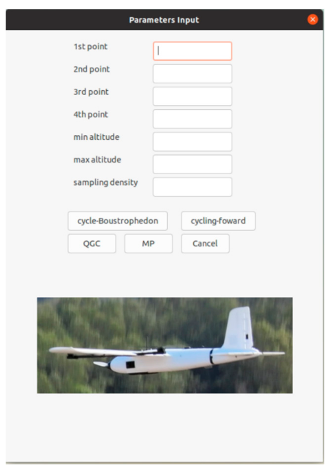
- In addition to the planner, design an easy-access user interface written in python script for users to interact with the module;
- To carry out simulations within the software-in-the-loop platform, in which the efficiency of our method is assessed by comparing it with the default software paths.
2. Materials and Methods
2.1. Coverage Path Generation for 3D Air Quality Profiling
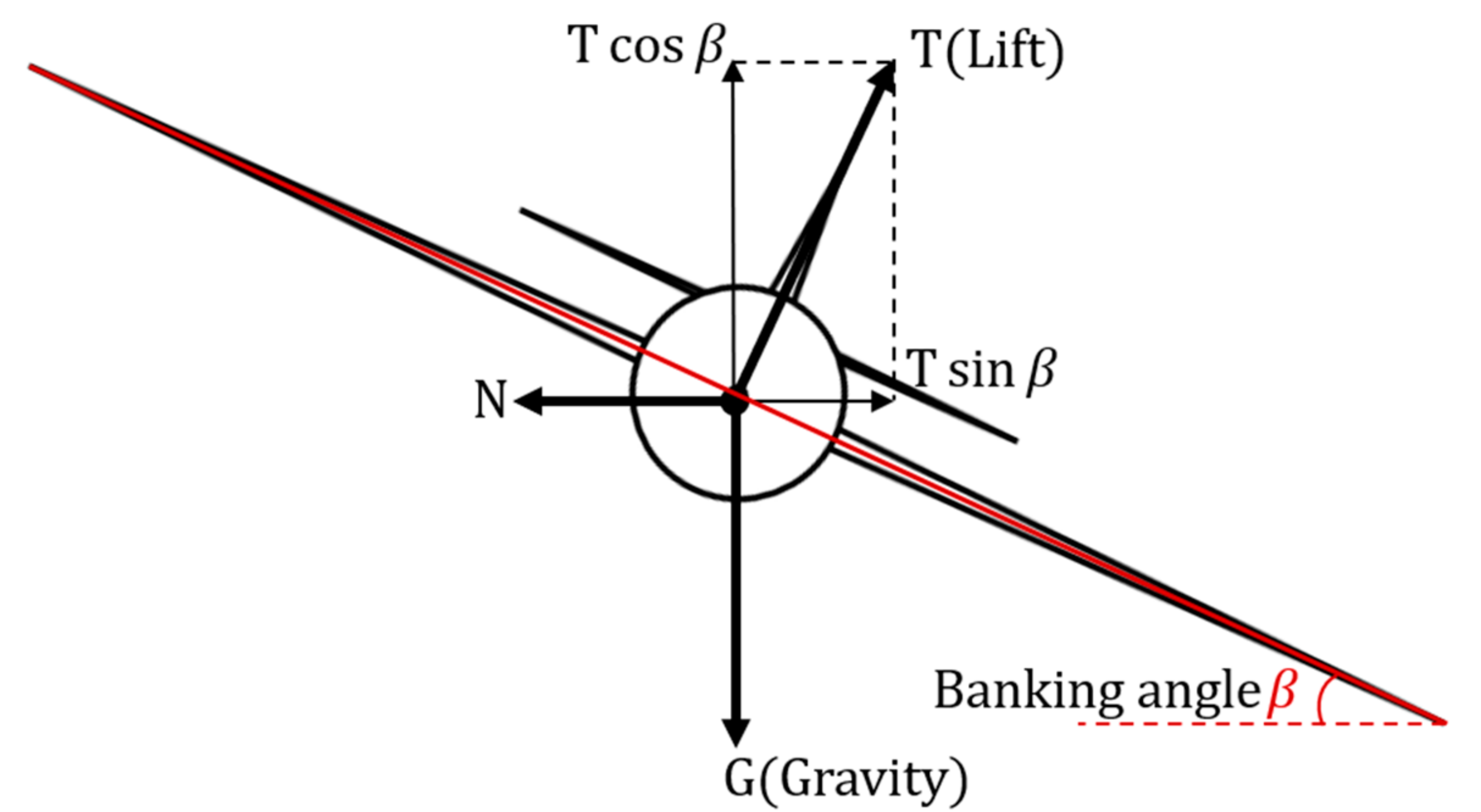
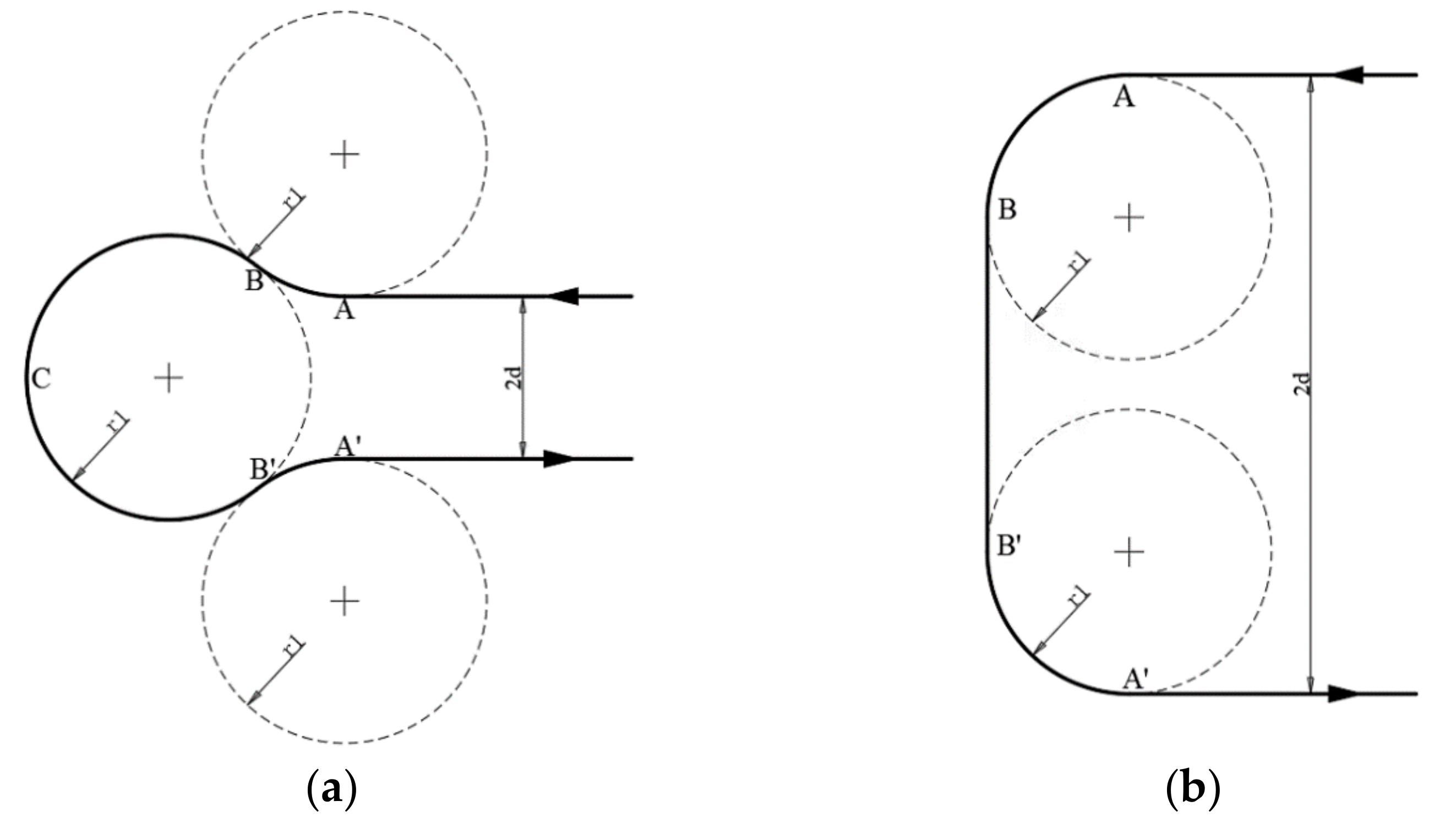
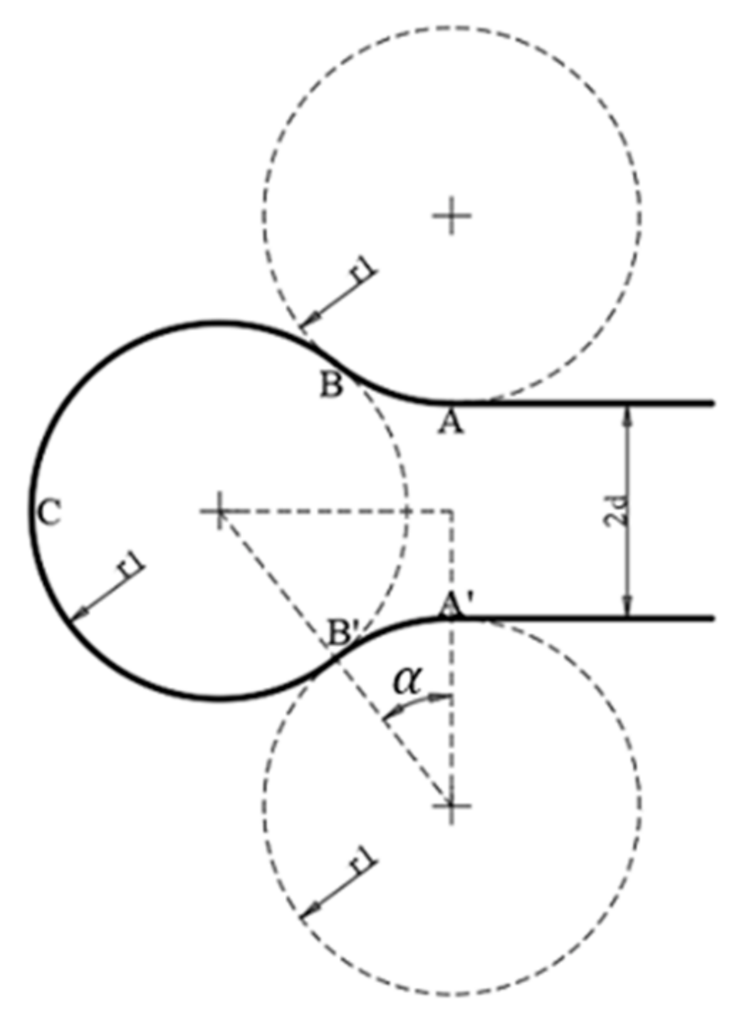
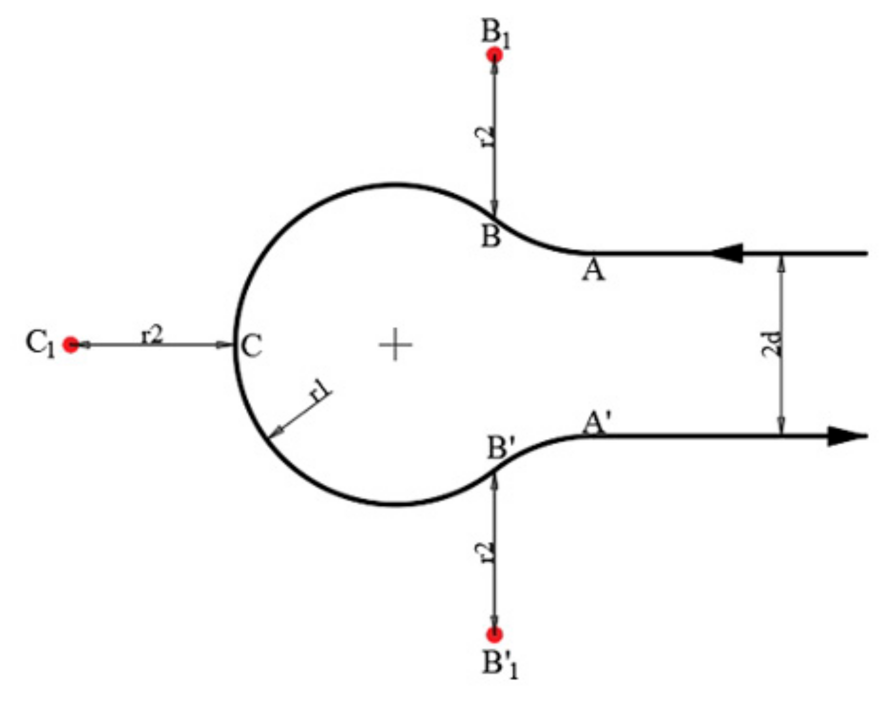
2.1.1. Coverage Path Planning Constraints for Fixed-Wing Aircrafts
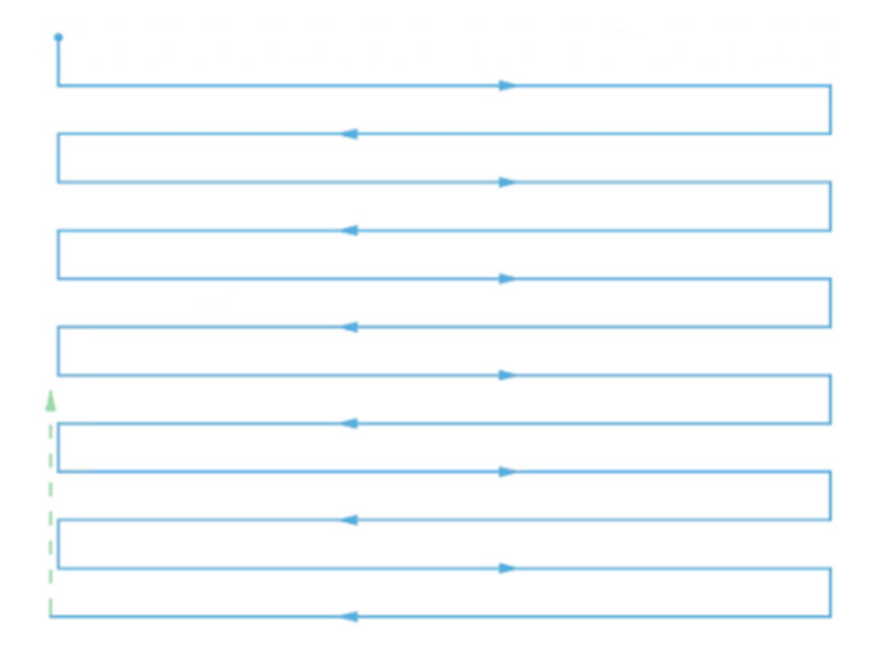
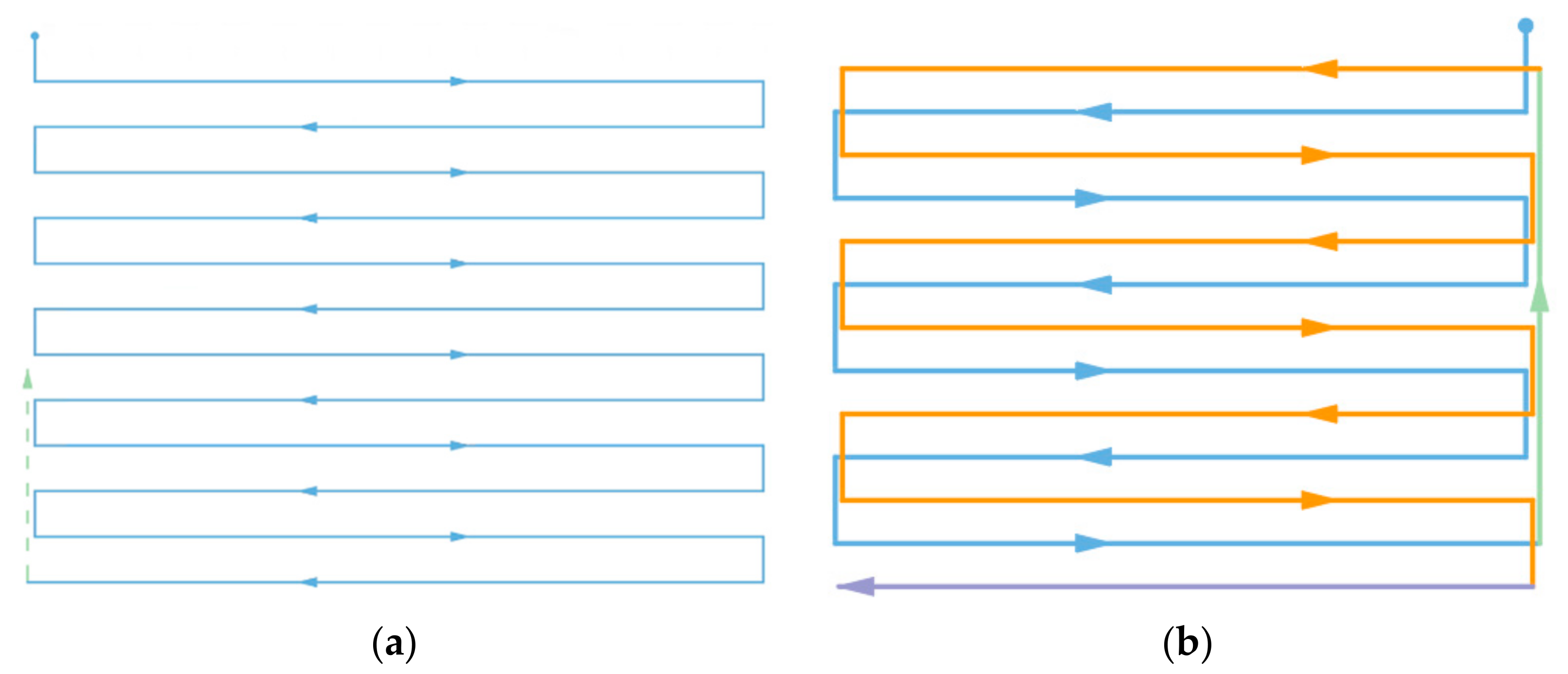
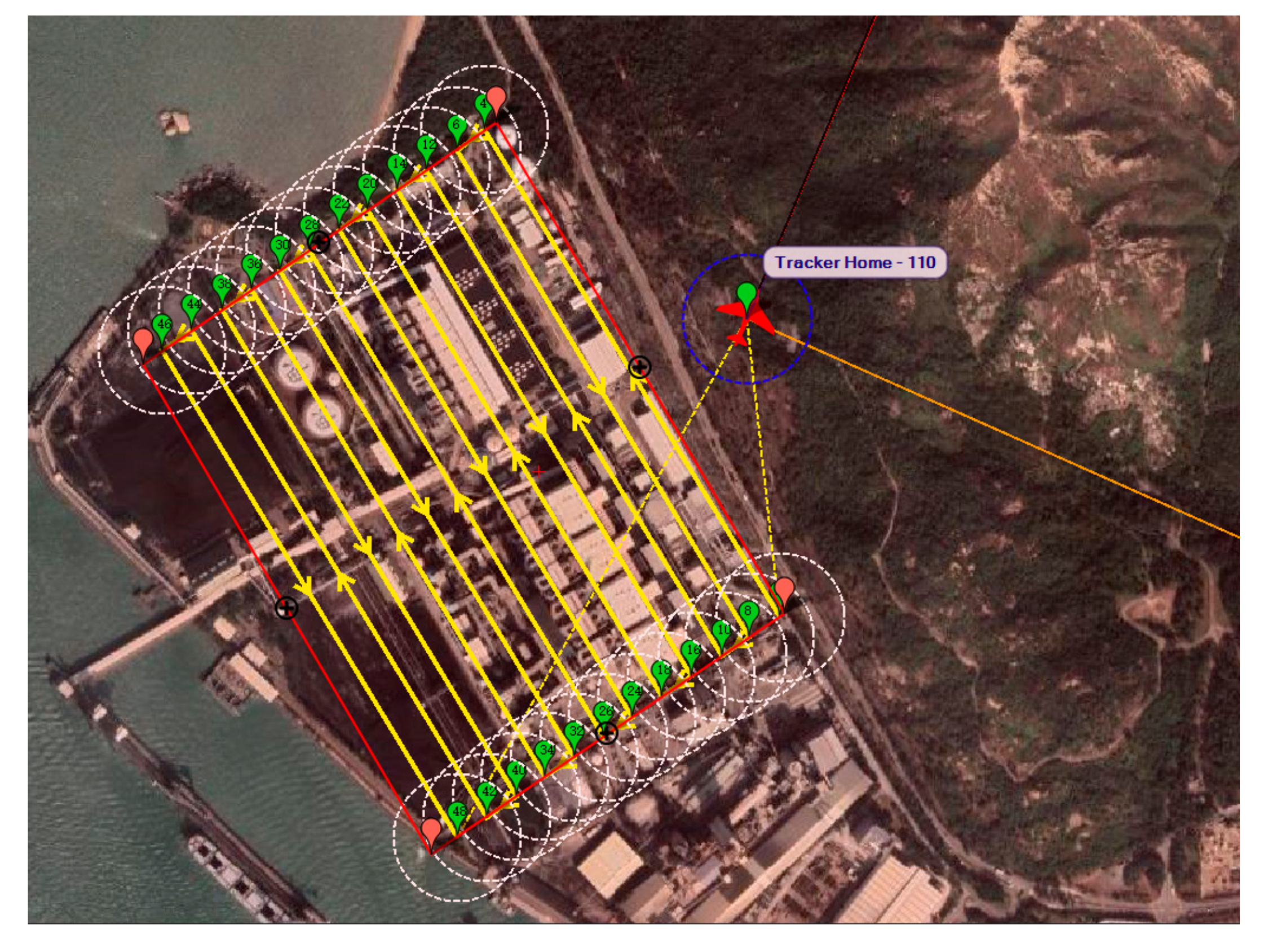
2.1.2. Cycle-Boustrophedon Path Planning
| Algorithm 1 Cycle-Boustrophedon Path Planning. |
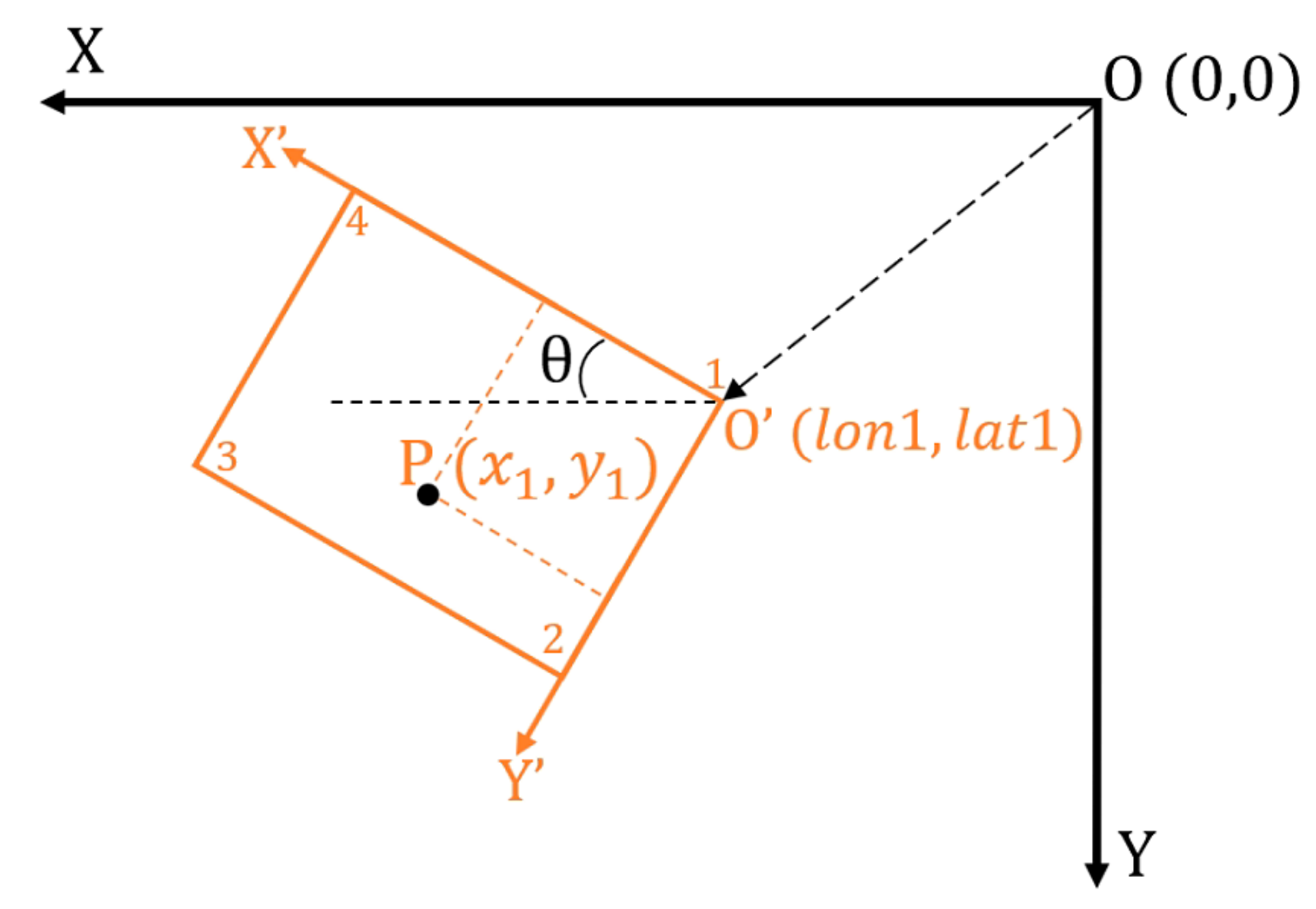
| Input: Home and takeoff location ROI vertices latitude and longitude Path separation distance in meters: ROI minimum altitude in meters: Number of layers: Layer separation distance in meters: Output: Readable waypoint file for GCS software Transfer vertices to local coordinates. Calculate LongEdge and ShortEdge ▷ Number of cycles required Initialize waypoint with home and takeoff location for to do for to do Add ABB’A’CDD’C’ location and height to waypoint ▷ Size of unit cycle is odd then ▷ Odd number means there is still half a cycle left to complete Add ABB’A’ location and height to waypoint ▷ Add the half of the last cycle end if Go to the center point of AA’ ▷ Do the second cycle at the same altitude for to do Add a unit cycle if is odd then Add a half of the last unit cycle end if end for end for end for Transfer waypoint to global coordinates Print to readable waypoint file |
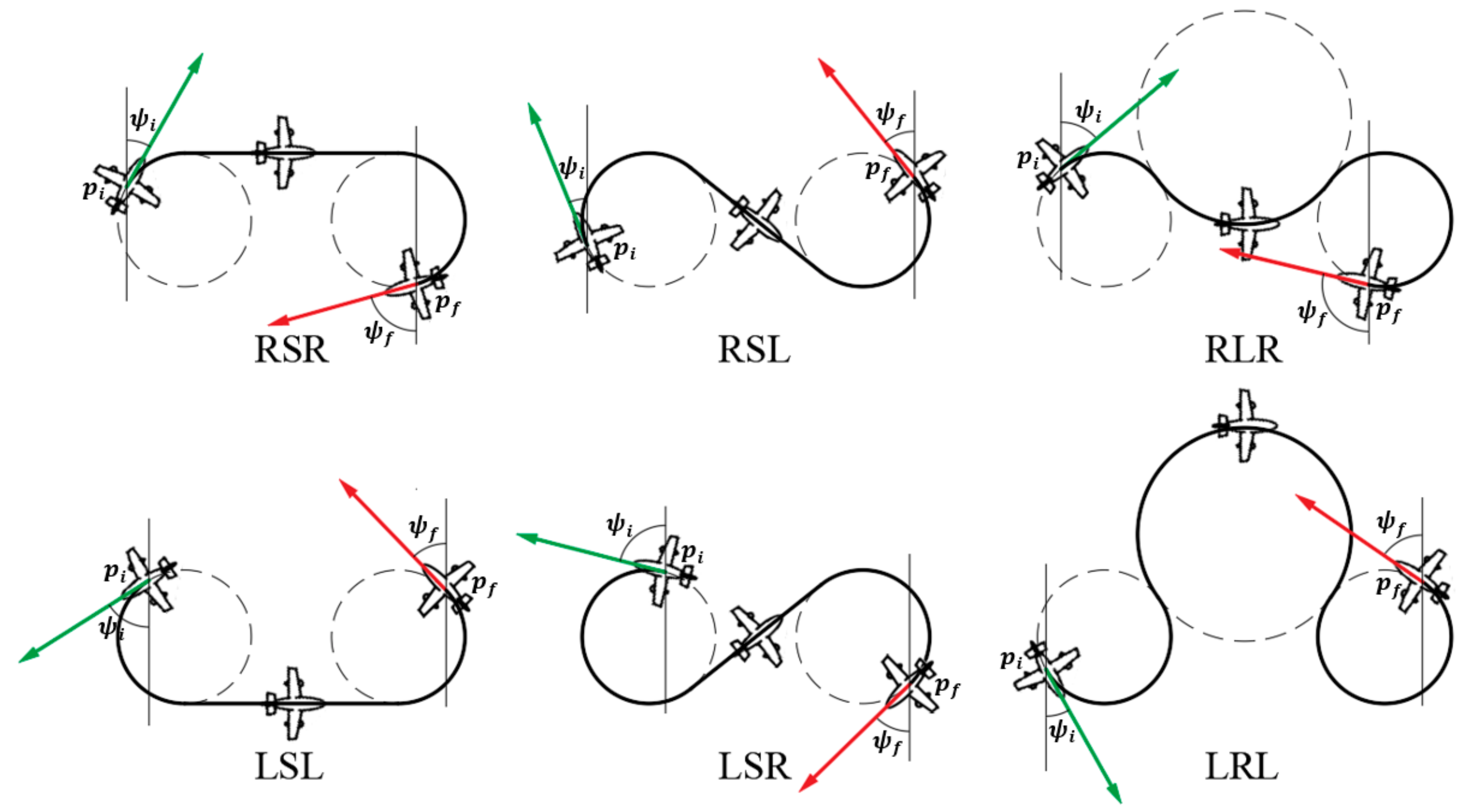
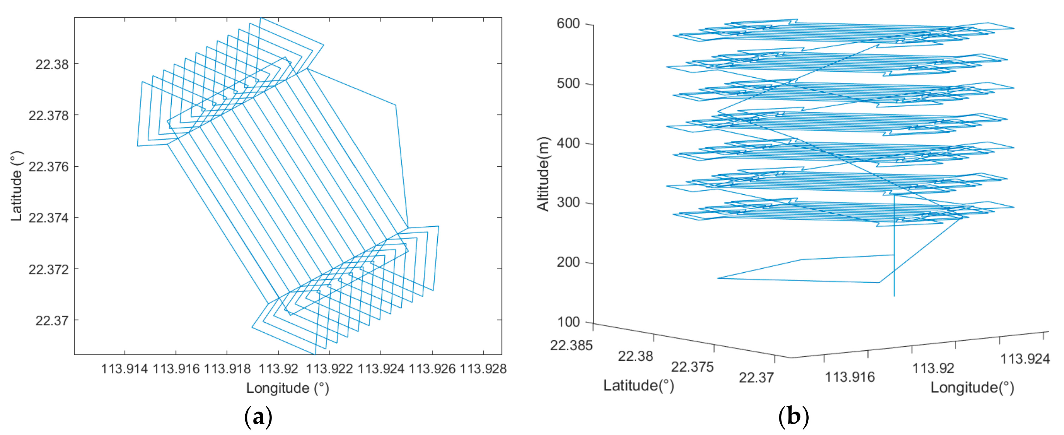
2.1.3. Circling-Forward Path Planning
| Algorithm 2 Circling-forward Path Planning. |
| Input: Home and takeoff location ROI vertices latitude and longitude Path separation distance in meters: ROI minimum altitude in meters: Number of layers: Layer separation distance in meters: Output: Readable waypoint file for GCS software Transfer vertices to local coordinates. Calculate LongEdge and ShortEdge ▷ Number of cycles required if is odd then ▷ Odd results in an uncovered path at middle of ROI ▷ Round up to even number end if ▷ Size of unit cycle ▷ Expand LongEdge for full coverage Initialize waypoint with home and takeoff location for to do for to do Add BCDE location and height to waypoint Move unit cycle along BC by end for end for Transfer waypoint to global coordinates Print to readable waypoint file |
2.2. Secure Return to Launch Path Generation
| Algorithm 3 Return to Launch Path Generation. |
|
Cycling path completed. while do ▷ θ is fixed glide angle Add next ROI vertex location and height to waypoint end while Add launch location to waypoint Transfer to quadrotor mode and land |
2.3. Easy-Access User Interface
2.4. Ground Control Station Software
3. Simulation Experiment
3.1. Auto-Grid Paths
3.1.1. Auto-Grid Paths in Simulation Platform 1
3.1.2. Auto-Grid Paths in Simulation Platform 2
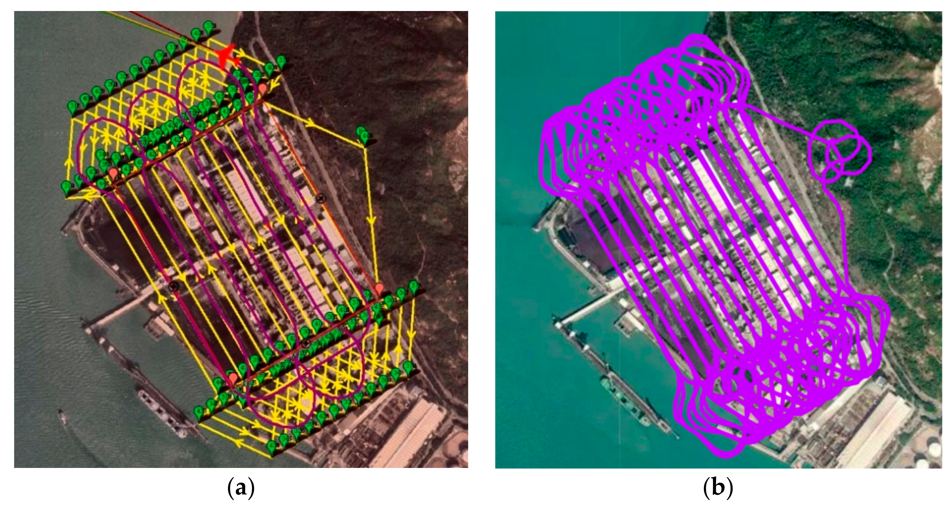
3.2. Cycle-Boustrophedon Path
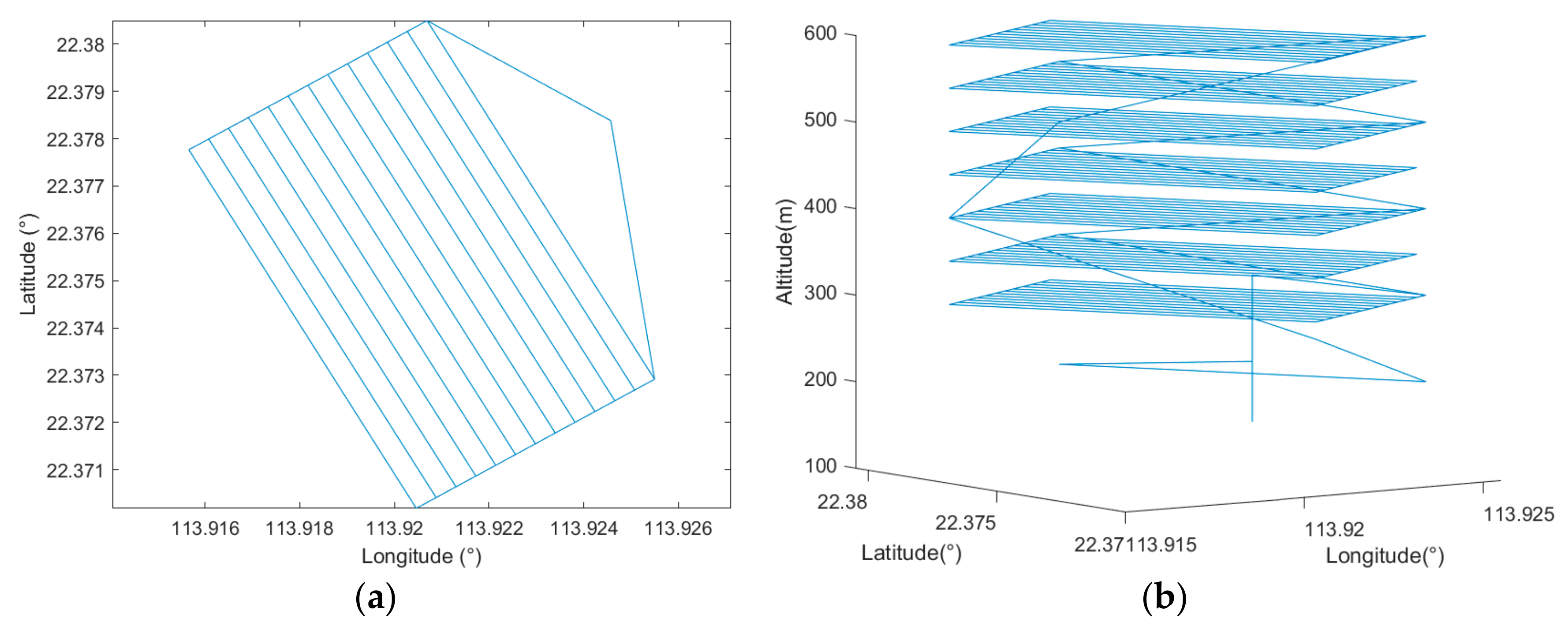
3.2.1. Cycle-Boustrophedon Path in Simulation Platform 1
3.2.2. Cycle-Boustrophedon Path in Simulation Platform 2
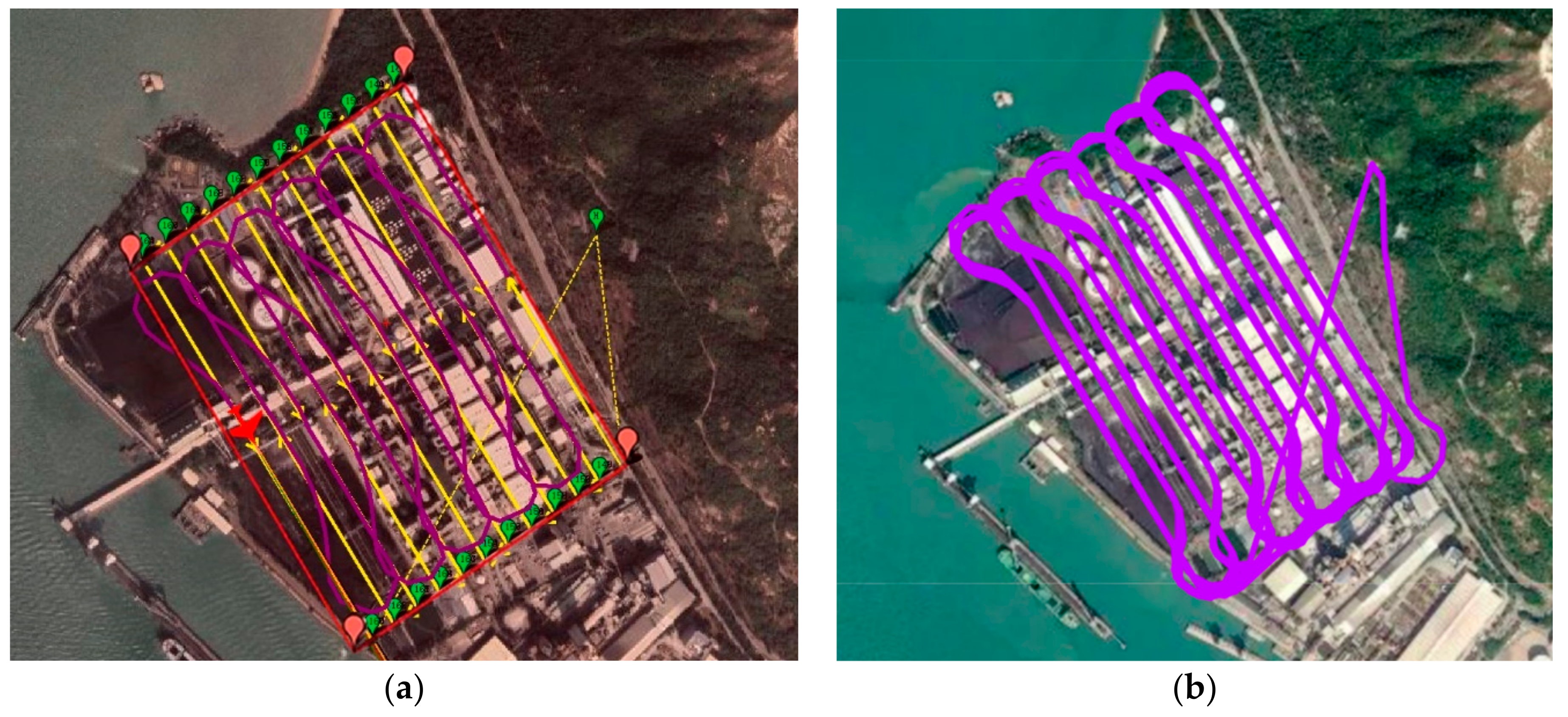
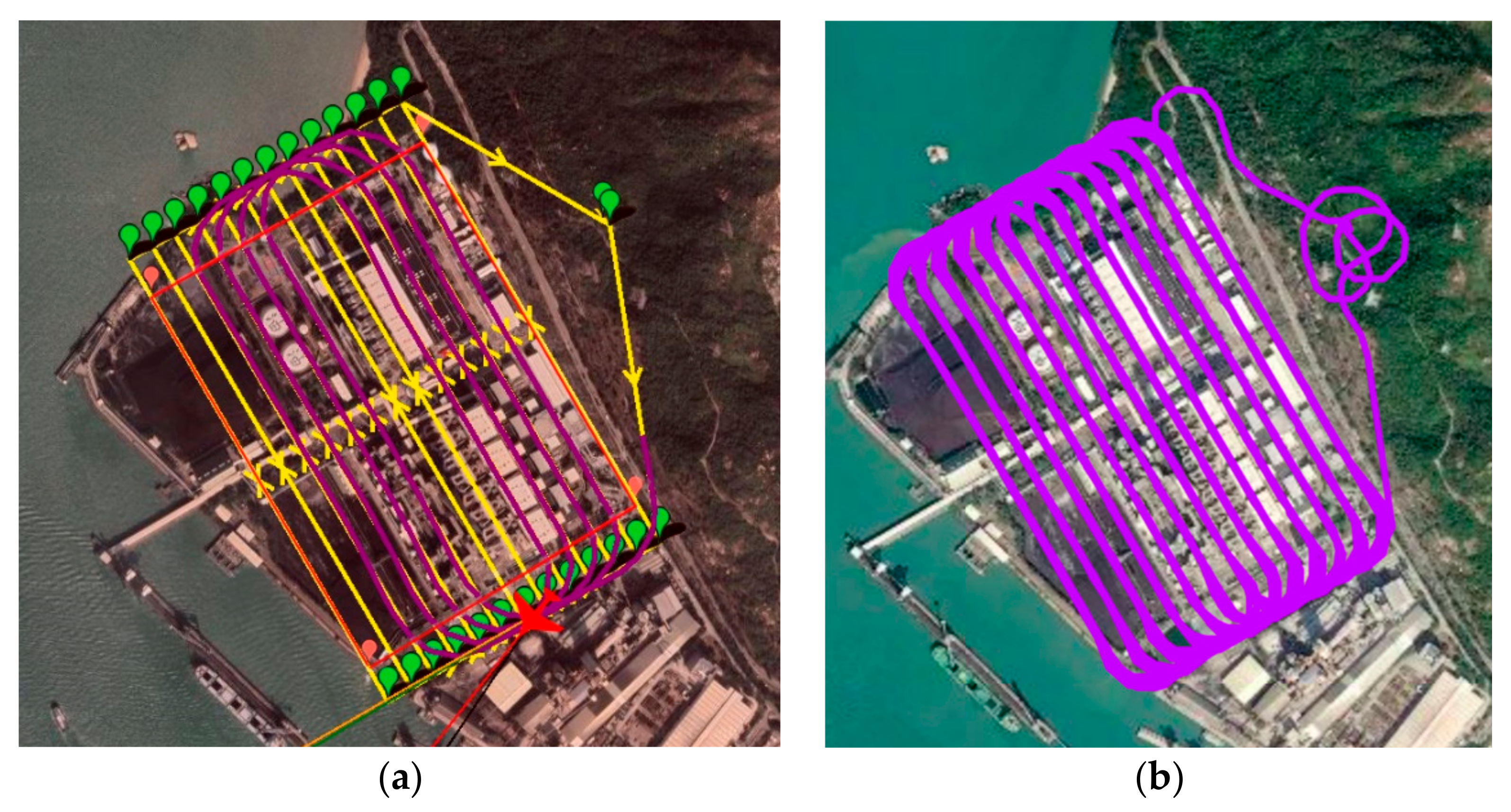
3.3. Circling-Forward Path Planner
3.3.1. Circling-Forward Path Planner in Simulation Platform 1
3.3.2. Circling-Forward Path Planner in Simulation Platform 2
3.4. Results and Discussion
3.4.1. Coverage Rate of ROI
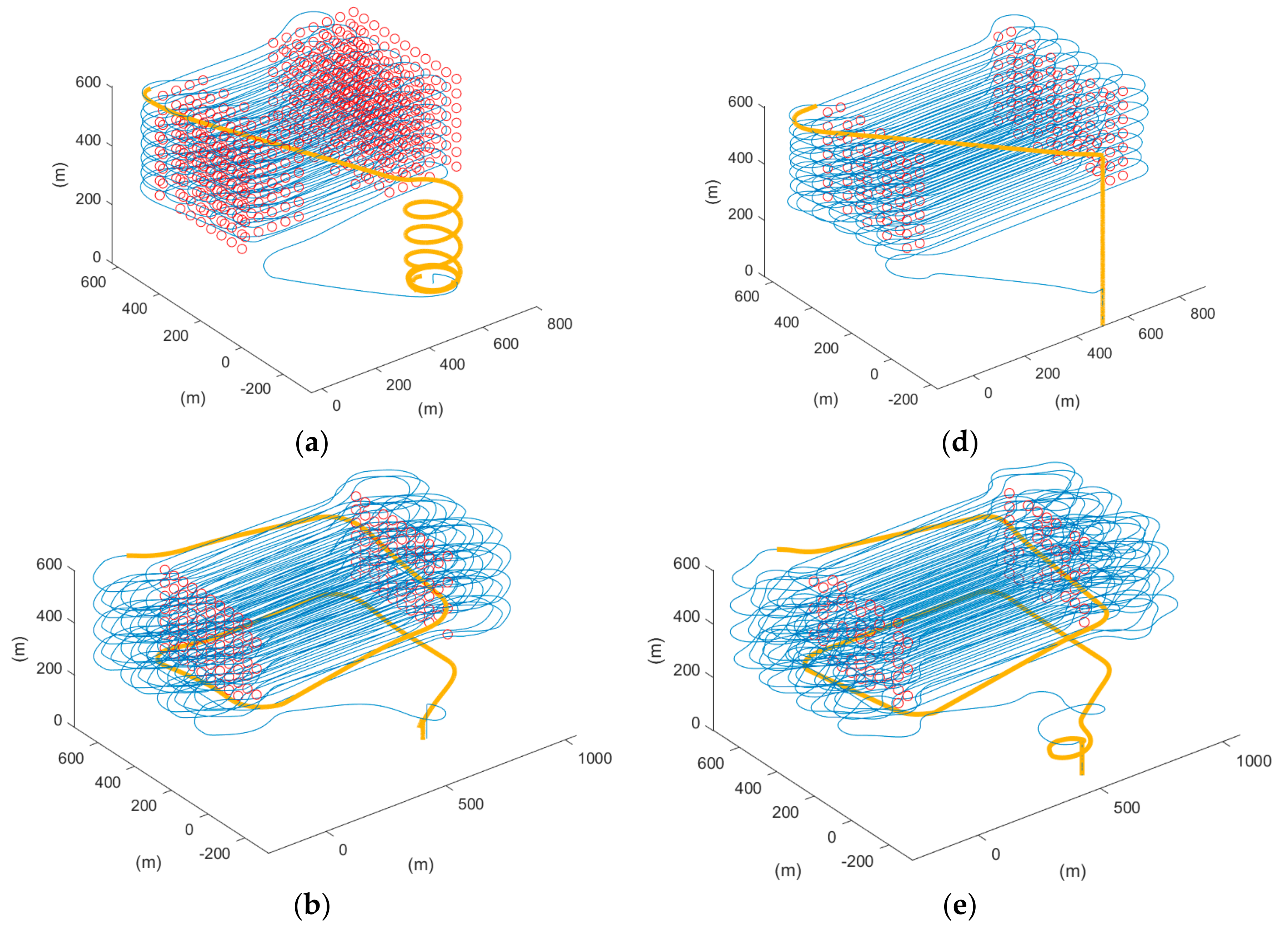
3.4.2. Comparison between Cycle-Boustrophedon and Circling-Forward
3.4.3. Duration and Distance of Different Paths
3.4.4. Return to Launch Paths
4. Conclusions
Author Contributions
Funding
Institutional Review Board Statement
Informed Consent Statement
Data Availability Statement
Conflicts of Interest
References
- Li, X.; Jin, L.; Kan, H. Air pollution: A global problem needs local fixes. Nature 2019, 570, 437–439. [Google Scholar] [CrossRef] [PubMed] [Green Version]
- Villa, T.F.; Gonzalez, F.; Miljievic, B.; Ristovski, Z.D.; Morawska, L. An overview of small unmanned aerial vehicles for air quality measurements: Present applications and future prospectives. Sensors 2016, 16, 1072. [Google Scholar] [CrossRef] [PubMed] [Green Version]
- Environmental Protection Department. Environmental Protection Interactive Centre. Available online: https://cd.epic.epd.gov.hk/EPICDI/air/station/?lang=en (accessed on 2 March 2022).
- Lambey, V.; Prasad, A. A review on air quality measurement using an unmanned aerial vehicle. Water Air Soil Pollut. 2021, 232, 109. [Google Scholar] [CrossRef]
- Karion, A.; Sweeney, C.; Wolter, S.; Newberger, T.; Chen, H.; Andrews, A.; Kofler, J.; Neff, D.; Tans, P. Long-term greenhouse gas measurements from aircraft. Atmos. Meas. Tech. 2013, 6, 511–526. [Google Scholar]
- Wich, S.; Koh, L.P. Conservation drones. GIM Int. 2012, 26, 29–33. [Google Scholar]
- Li, C.; Hsu, N.C.; Tsay, S.-C. A study on the potential applications of satellite data in air quality monitoring and forecasting. Atmos. Environ. 2011, 45, 3663–3675. [Google Scholar] [CrossRef]
- Engel-Cox, J.A.; Hoff, R.M.; Haymet, A. Recommendations on the use of satellite remote-sensing data for urban air quality. J. Air Waste Manag. Assoc. 2004, 54, 1360–1371. [Google Scholar] [CrossRef]
- Barnhart, R.K.; Marshall, D.M.; Shappee, E. Introduction to Unmanned Aircraft Systems; CRC Press: Boca Raton, FL, USA, 2021. [Google Scholar]
- Gu, Q.; Michanowicz, D.R.; Jia, C. Developing a modular unmanned aerial vehicle (UAV) platform for air pollution profiling. Sensors 2018, 18, 4363. [Google Scholar]
- Zhou, F.; Gu, J.; Chen, W.; Ni, X. Measurement of SO2 and NO2 in ship plumes using rotary unmanned aerial system. Atmosphere 2019, 10, 657. [Google Scholar] [CrossRef] [Green Version]
- Araujo, J.O.; Valente, J.; Kooistra, L.; Munniks, S.; Peters, R.J. Experimental flight patterns evaluation for a UAV-based air pollutant sensor. Micromachines 2020, 11, 768. [Google Scholar] [CrossRef]
- Jumaah, H.J.; Kalantar, B.; Halin, A.A.; Mansor, S.; Ueda, N.; Jumaah, S.J. Development of UAV-based PM2.5 monitoring system. Drones 2021, 5, 60. [Google Scholar] [CrossRef]
- Alvarado, M.; Gonzalez, F.; Fletcher, A.; Doshi, A. Towards the development of a low cost airborne sensing system to monitor dust particles after blasting at open-pit mine sites. Sensors 2015, 15, 19667–19687. [Google Scholar] [CrossRef] [PubMed] [Green Version]
- Roldán, J.J.; Joossen, G.; Sanz, D.; Del Cerro, J.; Barrientos, A. Mini-UAV based sensory system for measuring environmental variables in greenhouses. Sensors 2015, 15, 3334–3350. [Google Scholar] [CrossRef] [PubMed] [Green Version]
- Neumann, P.P. Gas Source Localization and Gas Distribution Mapping with a Micro-Drone; Bundesanstalt für Materialforschung und-Prüfung (BAM): Berlin, Germany, 2013. [Google Scholar]
- Gerhardt, N.; Clothier, R.; Wild, G.; Mohamed, A.; Petersen, P.; Watkins, S. Analysis of inlet flow structures for the integration of a remote gas sensor on a multi-rotor unmanned aircraft system. In Proceedings of the Fourth Australasian Unmanned Systems Conference (ACUS), Melbourne, Australia, 15–16 December 2014; pp. 1–6. [Google Scholar]
- Xu, A.; Viriyasuthee, C.; Rekleitis, I. Optimal complete terrain coverage using an unmanned aerial vehicle. In Proceedings of the International Conference on Robotics and Automation, Shanghai, China, 9–13 May 2011; pp. 2513–2519. [Google Scholar]
- Yasutomi, F.; Yamada, M.; Tsukamoto, K. Cleaning robot control. In Proceedings of the International Conference on Robotics and Automation, Philadelphia, PA, USA, 24–29 April 1988; pp. 1839–1841. [Google Scholar]
- Di Franco, C.; Buttazzo, G. Coverage path planning for UAVs photogrammetry with energy and resolution constraints. J. Intell. Robot. Syst. 2016, 83, 445–462. [Google Scholar] [CrossRef]
- Bosse, M.; Nourani-Vatani, N.; Roberts, J. Coverage algorithms for an under-actuated car-like vehicle in an uncertain environment. In Proceedings of the International Conference on Robotics and Automation, Roma. Italy, 10–14 April 2007; pp. 698–703. [Google Scholar]
- Galceran, E.; Carreras, M. A survey on coverage path planning for robotics. Robot. Auton. Syst. 2013, 61, 1258–1276. [Google Scholar] [CrossRef] [Green Version]
- Arkin, E.M.; Hassin, R. Approximation algorithms for the geometric covering salesman problem. Discret. Appl. Math. 1994, 55, 197–218. [Google Scholar] [CrossRef] [Green Version]
- Arkin, E.M.; Fekete, S.P.; Mitchell, J.S. Approximation algorithms for lawn mowing and milling. Comput. Geom. 2000, 17, 25–50. [Google Scholar] [CrossRef] [Green Version]
- Chung, S.-J.; Paranjape, A.A.; Dames, P.; Shen, S.; Kumar, V. A survey on aerial swarm robotics. IEEE Trans. Robot. 2018, 34, 837–855. [Google Scholar] [CrossRef] [Green Version]
- Simon, M.; Copăcean, L.; Popescu, C.; Cojocariu, L. 3D mapping of a village with a wingtraone vtol tailsiter drone using pix4d mapper. Res. J. Agric. Sci. 2021, 53, 228–237. [Google Scholar]
- Coombes, M.; Chen, W.-H.; Liu, C. Boustrophedon coverage path planning for UAV aerial surveys in wind. In Proceedings of the International Conference on Unmanned Aircraft Systems (ICUAS), Miami, FL, USA, 13–16 June 2017; pp. 1563–1571. [Google Scholar]
- Coombes, M.; Chen, W.-H.; Liu, C. Fixed wing UAV survey coverage path planning in wind for improving existing ground control station software. In Proceedings of the 37th Chinese Control Conference (CCC), Wuhan, China, 25–27 July 2018; pp. 9820–9825. [Google Scholar]
- Coombes, M.; Fletcher, T.; Chen, W.-H.; Liu, C. Optimal polygon decomposition for UAV survey coverage path planning in wind. Sensors 2018, 18, 2132. [Google Scholar] [CrossRef] [Green Version]
- Coombes, M.; Chen, W.-H.; Liu, C. Flight testing Boustrophedon coverage path planning for fixed wing UAVs in wind. In Proceedings of the International Conference on Robotics and Automation (ICRA), Montreal, QC, Canada, 20–24 May 2019; pp. 711–717. [Google Scholar]
- Paull, L.; Thibault, C.; Nagaty, A.; Seto, M.; Li, H. Sensor-driven area coverage for an autonomous fixed-wing unmanned aerial vehicle. IEEE Trans. Cybern. 2013, 44, 1605–1618. [Google Scholar] [CrossRef] [PubMed]
- Yu, X.; Li, C.; Yen, G.G. A knee-guided differential evolution algorithm for unmanned aerial vehicle path planning in disaster management. Appl. Soft Comput. 2021, 98, 106857. [Google Scholar] [CrossRef]
- Zhang, X.; Tian, Y.; Jin, Y. A knee point-driven evolutionary algorithm for many-objective optimization. IEEE Trans. Evol. Comput. 2014, 19, 761–776. [Google Scholar] [CrossRef]
- Ardupilot. ArduPilot Open Source Autopilot. 2018. Available online: https://ardupilot.org/ardupilot/index.html (accessed on 2 May 2022).
- Meier, L. MAVLink Micro Air Vehicle Communication Protocol; QGroundControl: 2017. Available online: http://qgroundcontrol.com (accessed on 2 May 2022).
- Rekleitis, I.; New, A.P.; Rankin, E.S.; Choset, H. Efficient boustrophedon multi-robot coverage: An algorithmic approach. Ann. Math. Artif. Intell. 2008, 52, 109–142. [Google Scholar] [CrossRef] [Green Version]
- Choset, H. Coverage of known spaces: The boustrophedon cellular decomposition. Auton. Robot. 2000, 9, 247–253. [Google Scholar] [CrossRef]
- Bui, X.-N.; Boissonnat, J.-D.; Soueres, P.; Laumond, J.-P. Shortest path synthesis for Dubins non-holonomic robot. In Proceedings of the International Conference on Robotics and Automation, San Diego, CA, USA, 8–13 May 1994; pp. 2–7. [Google Scholar]
- Lugo-Cárdenas, I.; Flores, G.; Salazar, S.; Lozano, R. Dubins path generation for a fixed wing UAV. In Proceedings of the International Conference on Unmanned Aircraft Systems (ICUAS), Orlando, FL, USA, 27–30 May 2014; pp. 339–346. [Google Scholar]
- Nguyen, K.D.; Ha, C. Development of hardware-in-the-loop simulation based on gazebo and pixhawk for unmanned aerial vehicles. Int. J. Aeronaut. Space Sci. 2018, 19, 238–249. [Google Scholar] [CrossRef]


| Simulation Platform 1 | Simulation Platform 2 | |
|---|---|---|
| Software Platform | Mission Planner SITL (software in the loop) Simulation [34] | Gazebo [40] |
| Firmware | ArduPilot | PX4 |
| Compared Paths | Auto-grid paths by Mission Planner | Auto-grid paths by QGroundControl |
| Parameters | Value |
|---|---|
| (max. air speed) | 30 m/s |
| (min. air speed) | 10 m/s |
| (banking angle) | 25 |
| (turning radius, assumed) | 87.5 m |
| (waypoint radius) | 90 m |
| d (sampling density) | 50 m |
| (vertex 1) | (113.9250, 22.3736) |
| (vertex 2) | (113.9202, 22.3705) |
| (vertex 3) | (113.9163, 22.3768) |
| (vertex 4) | (113.9211, 22.3798) |
| (max. altitude) | 600 m |
| (min. altitude) | 300 m |
| Scenario 1 | Scenario 2 | |
|---|---|---|
| Vertex 1 coordinates | (113.9250, 22.3736) | (114.2672861, 22.34372) |
| Vertex 2 coordinates | (113.9202, 22.3705) | (114.2711671, 22.3439472) |
| Vertex 3 coordinates | (113.9163, 22.3768) | (114.2713736, 22.3403549) |
| Vertex 4 coordinates | (113.9211, 22.3798) | (114.2674926, 22.3401327) |
| 600 | 500 | |
| 300 | 100 |
| Scenario 1 | Scenario 2 | |||
|---|---|---|---|---|
| MP SITL | QGC-Gazebo | MP SITL | QGC-Gazebo | |
| Auto-grid | 53.78% | 90.99% | 50.97% | 71.43% |
| Cycle-Boustrophedon | 89.69% | 93.89% | 83.07% | 87.65% |
| Circling-forward | 100% | 100% | 100% | 100% |
| Scenario 1 | ||||||||
|---|---|---|---|---|---|---|---|---|
| MP SITL | QGC-Gazebo | |||||||
| Flight duration | Flight distance | Flight duration | Flight distance | |||||
| Auto-grid | 4145 (s) | 89.11 (km) | 4716 (s) | 94.31 (km) | ||||
| Cycle-Boustrophedon | 5672 (s) | +36.84% | 110.6 (km) | +24.11% | 5317 (s) | +12.76% | 109.3 (km) | 15.89% |
| Circling-forward | 6168 (s) | +8.75% | 120.1 (km) | +8.58% | 5803 (s) | +9.13% | 119.3 (km) | 9.13% |
| Scenario 2 | ||||||||
| MP SITL | QGC-Gazebo | |||||||
| Flight duration | Flight distance | Flight duration | Flight distance | |||||
| Auto-grid | 2291 (s) | 38.44 (km) | 2842 (s) | 48.30 (km) | ||||
| Cycle-Boustrophedon | 3527 (s) | +53.95% | 54.82 (km) | +42.61% | 3077 (s) | +8.27% | 57.73 (km) | +19.52% |
| Circling-forward | 3768 (s) | +6.84% | 59.57 (km) | +8.67% | 3342 (s) | +8.61% | 62.85 (km) | +8.87% |
Publisher’s Note: MDPI stays neutral with regard to jurisdictional claims in published maps and institutional affiliations. |
© 2022 by the authors. Licensee MDPI, Basel, Switzerland. This article is an open access article distributed under the terms and conditions of the Creative Commons Attribution (CC BY) license (https://creativecommons.org/licenses/by/4.0/).
Share and Cite
Zhou, Q.; Lo, L.-Y.; Jiang, B.; Chang, C.-W.; Wen, C.-Y.; Chen, C.-K.; Zhou, W. Development of Fixed-Wing UAV 3D Coverage Paths for Urban Air Quality Profiling. Sensors 2022, 22, 3630. https://doi.org/10.3390/s22103630
Zhou Q, Lo L-Y, Jiang B, Chang C-W, Wen C-Y, Chen C-K, Zhou W. Development of Fixed-Wing UAV 3D Coverage Paths for Urban Air Quality Profiling. Sensors. 2022; 22(10):3630. https://doi.org/10.3390/s22103630
Chicago/Turabian StyleZhou, Qianyu, Li-Yu Lo, Bailun Jiang, Ching-Wei Chang, Chih-Yung Wen, Chih-Keng Chen, and Weifeng Zhou. 2022. "Development of Fixed-Wing UAV 3D Coverage Paths for Urban Air Quality Profiling" Sensors 22, no. 10: 3630. https://doi.org/10.3390/s22103630